This document outlines a lecture on continuous random variables and their probability distributions. It introduces probability density functions, cumulative distribution functions, and how to calculate the mean and variance of continuous random variables. It also covers specific continuous distributions like the uniform and normal distributions. Examples are provided to demonstrate calculating probabilities and standardizing normal random variables.

1. 9/28/2018
1
SBE 304: Bio-Statistics
Continuous Random Variables
and their Probability
Distributions
Dr. Ayman Eldeib
Systems & Biomedical
Engineering Department
Fall 2018
SBE 304: CRV - PDF
Outline
 Introduction
 Probability Distribution Functions
 Probability Density Function (PDF)
 Cumulative Distribution Function (CDF)
 The Mean and Variance of a Continuous Random
Variable
 Continuous Uniform Distribution
 Normal Distribution
 Normal Approximation to Binomial and Poisson
Distributions
 Continuity Correction to improve the approximation

2. 9/28/2018
2
SBE 304: CRV - PDF
A Discrete/Continuous
Random Variable
 A discrete random variable is a random variable with a finite
(or countable infinite) range. It is one that can assume only
distinct (whole number, 0, 1, 2, 3, 4, 5, 6, etc. ) Values.
Examples: Response with Yes - No values, number of
transmitted bits received in error, year (2010), etc.
 A continuous random variable is a random variable with an
interval (either finite or infinite) of real numbers for its range. It
is one that can assume any value over a continuous range of
possibilities.
Examples: temperature, weight, electrical current, length,
pressure, time, voltage, etc.
SBE 304: CRV - PDF
For a continuous random variable X, a probability density
function f(x) is a function such that,
f(x) ≥ 0
f(x)dx = 1
P(a ≤ X ≤ b) = f(x)dx = area under f(x) from a to b
for any a and b
∫
∞
-∞
Probability Density Function (PDF)
∫
b
a

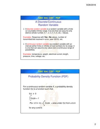
3. 9/28/2018
3
SBE 304: CRV - PDF
Based on the definition, for a continuous random variable X
and any value x, P(X = x) = 0, because every point has zero
width; i.e. zero area
However, in practice, when a particular x is observed,
such as 14.47, this result can be interpreted as the
rounded value that is actually in a range such as
14.465 ≤ x ≤ 14.475
P(x1 ≤ X ≤ x2) = P(x1 < X ≤ x2) = P(x1 ≤ X < x2) = P(x1 < X < x2)
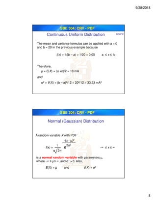
Cont’d
Probability Density Function (PDF)
SBE 304: CRV - PDF
Let the continuous random variable X denote the current
measured in a thin copper wire in milliamperes. Assume that
the range of X is [0, 20 mA], and assume that the probability
density function of X is f(x) = 0.05 for 0 ≤ x ≤ 20. What is the
probability that a current measurement is less than 10
milliamperes?
∫
10
0
P( X < 10)= f(x)dx = 0.05 dx = 0.5∫
10
0
What is the probability that a current measurement is between 5 and 20
milliamperes?
∫ ∫
20
P( 5 < X < 20)= f(x)dx = 0.05 dx = 0.75
20
5 5
Cont’d
Probability Density Function (PDF)

4. 9/28/2018
4
SBE 304: CRV - PDF
Cumulative Distribution Function
The cumulative distribution function of a continuous
random variable X, denoted as F(x), is
F(x) = P(X ≤ x) = f(u)du
for -∞ < x < ∞
-∞
x
∫
The probability density function of a continuous random
variable can be determined from the cumulative
distribution function by differentiating as long as the
derivative exists.
f(x) = dF(x)/dx
SBE 304: CRV - PDF
For the copper current measurement in the previous
example, the cumulative distribution function of the random
variable X consists of three expressions:
F(x) =
0 x < 0
0.05x 0 ≤ x < 20
1 20 ≤ x
Cont’dCumulative Distribution Function

5. 9/28/2018
5
SBE 304: CRV - PDF
Let the cumulative distribution function of a random variable Y be:
Example










<≤







<<





≤
=
otherwise
y
y
y
y
y
yF
,1
,42,
16
,20,
8
,0,0
)( 2
a. Find the probability density function of Y










<≤=







<<=





≤
=
otherwise
y
yy
dy
d
y
y
dy
d
y
yf
0
42
816
20
8
1
8
00
)( 2
b. Find P(1 ≤ Y ≤ 3) ( ) ( ) ( )1331 FFYP −=≤≤ 4375.0
16
7
16
2
16
9
==−=
c. Find P(1 ≤ Y < 3) Same result as (b)
Cont’dCumulative Distribution Function
SBE 304: CRV - PDF
Let the cumulative distribution function of a random variable Y be:
Example










<≤







<<





≤
=
otherwise
y
y
y
y
y
yF
,1
,42,
16
,20,
8
,0,0
)( 2
d. Find P(Y ≥ 1.5)
e. Find P(Y ≥ 1 | Y ≤ 3)
( ) ( ) 8125.016/13
8
5.1
15.115.1 ==−=−=≥ FYP
( ) ( )
( )
( )
( )
( ) ( )
( )
778.0
9
7
16
9
16
7
3
13
3
31
3
31
31 ===
−
=
≤
≤≤
=
≤
≤∩≥
=≤≥
F
FF
YP
YP
YP
YYP
YYP
Cont’dCumulative Distribution Function

6. 9/28/2018
6
SBE 304: CRV - PDF
The Mean and variance of a Continuous
Random Variable
The mean or expected value of the continuous random
variable X with PDF f(x), denoted as µ or E(X), is
µ = E(X) = x f(x)dx∫
∞
-∞
The variance of X, denoted as σ2 or V(X), is
σ2 = V(X) = E[(X - µ)2] = (x - µ)2 f(x)dx = x2 f(x)dx - µ2
∫
∞
-∞
∫
∞
-∞
The standard deviation of X, denoted as σ = σ2
SBE 304: CRV - PDF
The Mean and variance of a Continuous
Random Variable
µ = E(X) = x f(x)dx = 0.05x2/2 = 10 mA∫
20
0
σ2 = V(X) = E[(X - µ)2] = (x - 10)2 f(x)dx
= x2 f(x)dx – 100 = 33.33 mA2
∫
20
0
∫
20
0
For the copper current measurement in the previous example,
the mean of X is
|
20
0

7. 9/28/2018
7
SBE 304: CRV - PDF
The Expected value of a Function of a
Continuous Random Variable
Let X be a continuous random variable with PDF f(x),
E(g(X)) = g(x)f(x)dx
In the special case that g(X) = aX +b for any constants a
and b, Then the expected value of g(X) is given by
E(g(X)) = aE(X) + b
∫
∞
-∞
SBE 304: CRV - PDF
Continuous Uniform Distribution
A random variable X has a continuous uniform distribution
if
f(x) = 1/(b – a), a ≤ x ≤ b
µ = E(X) = (a +b)/2
Then,
and
σ2 = V(X) = (b – a)2/12

8. 9/28/2018
8
SBE 304: CRV - PDF
The mean and variance formulas can be applied with a = 0
and b = 20 in the previous example because
f(x) = 1/(b – a) = 1/20 = 0.05 a ≤ x ≤ b
µ = E(X) = (a +b)/2 = 10 mA
Therefore,
and
σ2 = V(X) = (b – a)2/12 = 202/12 = 33.33 mA2
Cont’dContinuous Uniform Distribution
SBE 304: CRV - PDF
Normal (Gaussian) Distribution
A random variable X with PDF
f(x) = e -∞ ≤ x ≤ ∞
σ 2π
1 2σ2
-(x - µ)2
is a normal random variable with parameters µ,
where -∞ ≤ µ≤ ∞, and σ > 0. Also,
E(X) = µ and V(X) = σ2

9. 9/28/2018
9
SBE 304: CRV - PDF
Normal (Gaussian) Distribution
 µ ± σ contains about
68% of the
measurements.
 µ ± 2σ contains
about 95% of the
measurements.
 µ ± 3σ contains
almost all
measurements.
Empirical Rule
Probability Density Function
normal (or Gaussian) distribution
SBE 304: CRV - PDF
The standard normal distribution is a special case of the
normal distribution. It is the distribution that occurs when a
normal random variable has a mean of zero and a standard
deviation of one.
The normal random variable of a standard normal distribution
is called a standard score or a z-score.
Standard Normal Distribution
E(X) = µ = 0 and V(X) = σ2 = 1

10. 9/28/2018
10
SBE 304: CRV - PDF
Standard Normal Distribution Table
A standard normal distribution table shows a cumulative
probability associated with a particular z-score.
Φ(z) = P(Z ≤ z)
Table rows show the whole number and tenths place of the z-
score. Table columns show the hundredths place. The
cumulative probability (often from minus infinity to the z-
score) appears in the cell of the table.
SBE 304: CRV - PDF
z 0.00 0.01 0.02 0.03 0.04 0.05 0.06 0.07 0.08 0.09
-3.0 0.0013 0.0013 0.0013 0.0012 0.0012 0.0011 0.0011 0.0011 0.0010 0.0010
... ... ... ... ... ... ... ... ... ... ...
-1.4 0.0808 0.0793 0.0778 0.0764 0.0749 0.0735 0.0722 0.0708 0.0694 0.0681
-1.3 0.0968 0.0951 0.0934 0.0918 0.0901 0.0885 0.0869 0.0853 0.0838 0.0823
-1.2 0.1151 0.1131 0.1112 0.1093 0.1075 0.1056 0.1038 0.1020 0.1003 0.0985
... ... ... ... ... ... ... ... ... ... ...
3.0 0.9987 0.9987 0.9987 0.9988 0.9988 0.9989 0.9989 0.9989 0.9990 0.9990
P(Z < -1.31) = 0.0951
Cont’dStandard Normal Distribution Table

11. 9/28/2018
11
SBE 304: CRV - PDF
P(Z > a) = 1 - P(Z < a)
P(a < Z < b) = P(Z < b) - P(Z < a)
This probability expression can be written as P(Z ≤ z) = 0.95.
Now, The Table is used in reverse. We search through the
probabilities to find the value that corresponds to 0.95. We do
not find 0.95 exactly; the nearest value is 0.95053,
corresponding to z = 1.65.
Find the value z such that P(Z > z) = 0.05
Cont’dStandard Normal Distribution Table
SBE 304: CRV - PDF
Normal Random Variable Standardization
Every normal random variable X can be transformed into a z-
score via the following equation:
Z = (X - μ) / σ
where X is a normal random variable, μ is the mean of X, and
σ is the standard deviation of X.

12. 9/28/2018
12
SBE 304: CRV - PDF
Mahmoud earned a score of 940 on a national
achievement test. The mean test score was 850 with a
standard deviation of 100. What proportion of students had
a higher score than Mahmoud ? (Assume that test scores
are normally distributed.)
z = (x - μ) / σ = (940 - 850) / 100 = 0.90
P(Z > 0.90) = 1 - P(Z < 0.90) = 1 - 0.8159 = 0.1841
Thus, we estimate that 18.41 percent of the students
tested had a higher score than Mahmoud.
Cont’d
Normal Random Variable Standardization
SBE 304: CRV - PDF
Normal Approximation to the Binomial
Distribution
If X is a binomial random variable,
is approximately a standard normal random variable.
The approximation is good for :
np > 5 and n(1- p) > 5
Z = (X - np) / sqrt(np(1 - p))

13. 9/28/2018
13
SBE 304: CRV - PDF
In a digital communication channel, assume that the number
of bits received in error can be modeled by a binomial
random variable, and assume that the probability that a bit is
received in error is 1 x 10-5. If 16 million bits are transmitted,
what is the probability that more than 150 errors occur?
Let the random variable X denote the number of errors.
Then X is a binomial random variable and
P(X > 150) = 1 - P(X ≤ 150) which is difficult to compute
Cont’d
Normal Approximation to the Binomial
Distribution
SBE 304: CRV - PDF
By using the normal approximation:
P(X > 150) = P(Z > -0.79) = P(Z < 0.79) = 0.785
Z = (X - np) / sqrt(np(1 - p))
z = (150 - 160) / sqrt(160(1 – 10-5)) = -0.79
Because np = (16 x 106)(1 x 10-5) = 160 and n(1 - p) is
much larger, the approximation is expected to work well
in this case.
Cont’d
Normal Approximation to the Binomial
Distribution

14. 9/28/2018
14
SBE 304: CRV - PDF
If X is a binomial random variable with parameters n and p,
and if x = 0, 1, 2, … , n, the continuity correction to
improve approximations obtained from the normal
distribution is
P(X ≤ x) = P(X ≤ x + 0.5) = P(Z ≤ (x + 0.5 - np) / sqrt(np(1 - p))
Continuity Correction
P(x ≤ X) = P(x - 0.5 ≤ X) = P((x - 0.5 - np) / sqrt(np(1 - p) ≤ Z)
and
~
~
Cont’d
Normal Approximation to the Binomial
Distribution
SBE 304: CRV - PDF
Normal Approximation to the Poisson
Distribution
If X is a Poisson random variable, with E(X) = V(X) = λ
is approximately a standard normal random variable.
The approximation is good for : λ > 5
Z = (X - λ) / sqrt(λ)

15. 9/28/2018
15
SBE 304: CRV - PDF
Exponential Random Variable
The random variable X that equals the distance between
successive counts of a Poisson process with mean λ > 0 is an
exponential random variable with parameter λ. The
probability density function of X is
f(x) = λ e –λx for 0 ≤ x < ∞
Also,
E(X) = µ = 1/ λ and V(X) = σ2 = 1/ λ2
SBE 304: CRV - PDF
For an exponential random variable X,
Lack of Memory Property
P(X < t1 + t2 | X > t1) = P(X < t2)
Cont’dExponential Random Variable

16. 9/28/2018
16
SBE 304: CRV - PDF
Erlang Random Variable
The random variable X that equals the interval length until
r counts occur in a Poisson process with mean λ > 0 has
an Erlang random variable with parameters λ and r.
The probability density function of X is
f(x) = for x > 0 and r = 1,2,...
λr xr-1e-λx
(r – 1)!
Also,
E(X) = µ = r/ λ and V(X) = σ2 = r/ λ2
SBE 304: CRV - PDF
Gamma Function
What if the parameter r of an Erlang random variable is
not an integer, but r > 0
The gamma function is
∫
∞
0
Г(r) = xr-1 e –x dx , for r > 0
Г(r) = (r – 1) Г(r - 1)
Г(1) = 0! = 1 Г(1/2) = π1/2

17. 9/28/2018
17
SBE 304: CRV - PDF
Gamma Random Variable
The random variable X with probability density function
f(x) = for x > 0
λr xr-1e-λx
Г(r)
Also,
E(X) = µ = r/ λ and V(X) = σ2 = r/ λ2
has a gamma random variable with parameters
λ > 0 and r > 0.
If r is an integer, X has an Erlang distribution
SBE 304: CRV - PDF
Joint Probability Distribution
In the study of probability, given two random variables X and
Y that are defined on the same probability space, the joint
distribution for X and Y defines the probability of events
defined in terms of both X and Y. In the case of only two
random variables, this is called a bivariate distribution, but
the concept generalizes to any number of random variables,
giving a multivariate distribution.

18. 9/28/2018
18
SBE 304: CRV - PDF
The joint probability density function of the continuous
random variables X and Y, denoted as fXY (x, y), satisfies:
0 ≤ fXY (x, y) ≤ 1 for all x and y
fXY (x, y) dx dy = 1
For any region R of two-dimensional space
P([X , Y] Є R) = fXY (x, y) dx dy
∫
∞
- ∞
∫
∞
- ∞
∫
R
∫
Cont’d
Joint Probability Distribution
SBE 304: CRV - PDF
For continuous random variables X and Y, check the
following:
Marginal Probability Distributions
Mean and Variance from Joint Distribution
Conditional Probability Distributions
Independence
Cont’d
Joint Probability Distribution