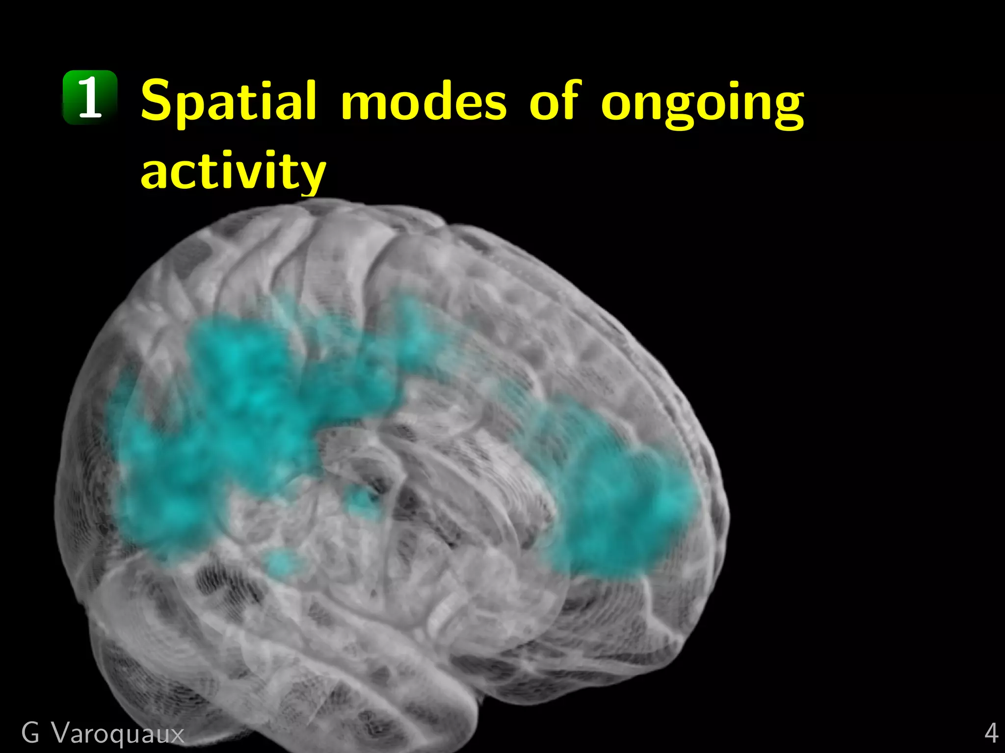
Download as PDF, PPTX
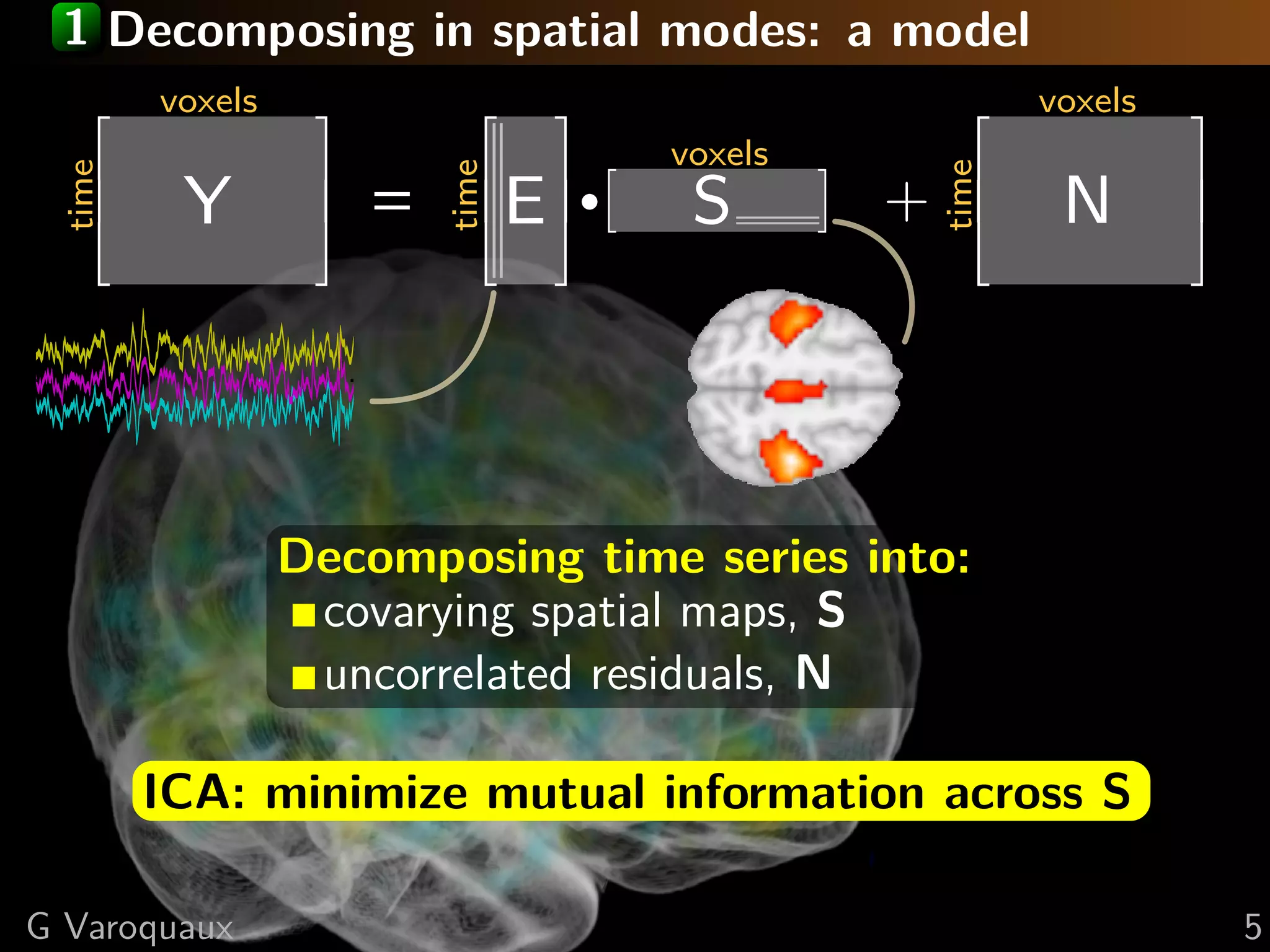
![1 ICA on multiple subjects: group ICA
Estimate common spatial maps S:
voxels voxels
voxels
Y
1
E
1
· S + N
1
time
time
time
=
·
· ·
· ·
·
s s s
Y E · S + N
time
time
time
=
G Varoquaux [Calhoun HBM 2001] 6](https://image.slidesharecdn.com/slides-110908185048-phpapp02/75/Learning-and-comparing-multi-subject-models-of-brain-functional-connecitivity-7-2048.jpg)
![1 ICA on multiple subjects: group ICA
Estimate common spatial maps S:
voxels voxels
voxels
Y
1
E
1
· S + N
1
time
time
time
=
·
· ·
· ·
·
s s s
Y E · S + N
time
time
time
=
Concatenate images, minimize norm of residuals
Corresponds to fixed-effects modeling:
i.i.d. residuals Ns
G Varoquaux [Calhoun HBM 2001] 6](https://image.slidesharecdn.com/slides-110908185048-phpapp02/75/Learning-and-comparing-multi-subject-models-of-brain-functional-connecitivity-8-2048.jpg)
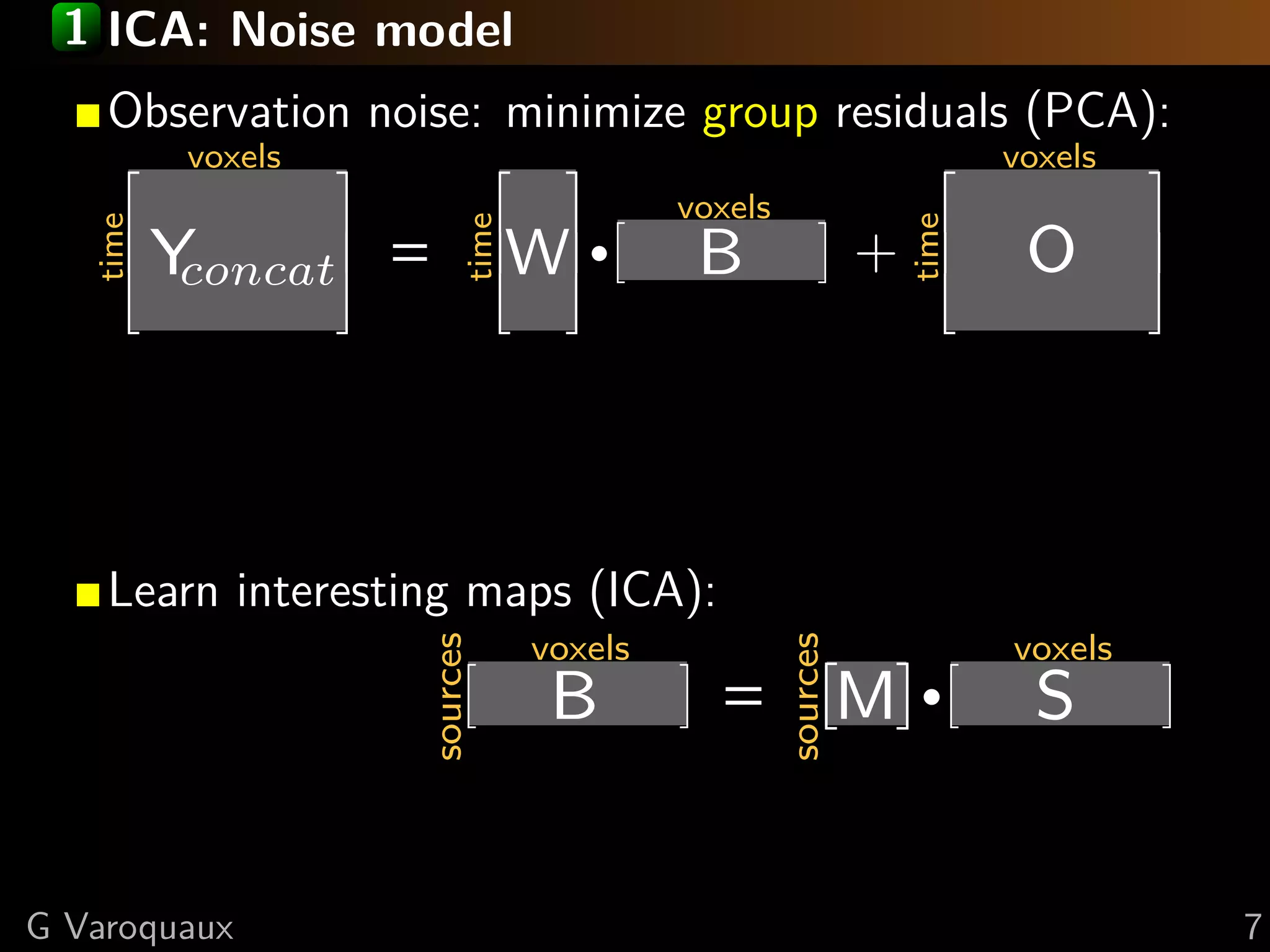
![1 CanICA: random effects model
Observation noise: minimize subject residuals (PCA):
voxels voxels
Subject
voxels
Y W · P + Os
time
time
time
s = s s
Select signal similar across subjects (CCA):
voxels
P1
Group
voxels
·
subjects
sources
.
.
. = Λ· B + R
Ps
Learn interesting maps (ICA):
voxels voxels
·
sources
sources
B = M S
G Varoquaux [Varoquaux NeuroImage 2010] 8](https://image.slidesharecdn.com/slides-110908185048-phpapp02/75/Learning-and-comparing-multi-subject-models-of-brain-functional-connecitivity-10-2048.jpg)
![1 CanICA: experimental validation
Reproducibility across controls groups
no CCA CanICA MELODIC
.36 (.02) .72 (.05) .51 (.04)
Qualitative observation: less ’noise’ components
G Varoquaux [Varoquaux NeuroImage 2010] 9](https://image.slidesharecdn.com/slides-110908185048-phpapp02/75/Learning-and-comparing-multi-subject-models-of-brain-functional-connecitivity-11-2048.jpg)
![1 Noise in the ICA maps
How to describe noise versus signal?
⇓ ⇓
Blobs standing out
Background noise
G Varoquaux [Varoquaux ISBI 2010] 10](https://image.slidesharecdn.com/slides-110908185048-phpapp02/75/Learning-and-comparing-multi-subject-models-of-brain-functional-connecitivity-12-2048.jpg)
![1 Noise in the ICA maps
How to describe noise versus signal?
Joint
distribution:
Blobs standing out = long-tailed distribution
Background noise = isotropic central mode
G Varoquaux [Varoquaux ISBI 2010] 10](https://image.slidesharecdn.com/slides-110908185048-phpapp02/75/Learning-and-comparing-multi-subject-models-of-brain-functional-connecitivity-13-2048.jpg)
![1 Noise in the ICA maps
How to describe noise versus signal?
⇓ ⇓
Thresholding
Joint
distribution:
G Varoquaux [Varoquaux ISBI 2010] 10](https://image.slidesharecdn.com/slides-110908185048-phpapp02/75/Learning-and-comparing-multi-subject-models-of-brain-functional-connecitivity-14-2048.jpg)
![1 ICA as a sparse decomposition
⇒
voxels
·( voxels voxels
(
sources
sources
B = M S + Q
Interesting sources S are sparse
Q: Gaussian noise
Thresholding ICA = sparse recovery
Experimental validation: on sub-sampled signal:
more robust than other approaches
G Varoquaux [Varoquaux ISBI 2010] 11](https://image.slidesharecdn.com/slides-110908185048-phpapp02/75/Learning-and-comparing-multi-subject-models-of-brain-functional-connecitivity-15-2048.jpg)
![1 The group-level ICA maps
Visual system
map 0, reproducibility: 0.54
-74
V1 0 9
map 1, reproducibility: 0.52
-91
V1-V2 3 -3
map 3, reproducibility: 0.47
-80 40 4
extrastriate
map 25, reproducibility: 0.34
-78 -30 24
superior parietal
G Varoquaux [Varoquaux NeuroImage 2010] 12](https://image.slidesharecdn.com/slides-110908185048-phpapp02/75/Learning-and-comparing-multi-subject-models-of-brain-functional-connecitivity-16-2048.jpg)
![1 The group-level ICA maps
Motor system
map 4, reproducibility: 0.47
part of
-25 -1 62
motor
map 21, reproducibility: 0.36
part of
-21 -42 54
motor
map 32, reproducibility: 0.30
part of
-8 -54 29
motor
G Varoquaux [Varoquaux NeuroImage 2010] 12](https://image.slidesharecdn.com/slides-110908185048-phpapp02/75/Learning-and-comparing-multi-subject-models-of-brain-functional-connecitivity-17-2048.jpg)
![1 The group-level ICA maps
Frontal structures
map 18, reproducibility: 0.37 map 23, reproducibility: 0.35
dorsal
43
frontal -30 28 10
medial wall
0 54
map 29, reproducibility: 0.31
21 pre-frontal 0 24
map 39, reproducibility: 0.26 map 37, reproducibility: 0.28
part of part of
21 prefronto-insular -34 -8 15 prefronto-insular -42 -3
G Varoquaux [Varoquaux NeuroImage 2010] 12](https://image.slidesharecdn.com/slides-110908185048-phpapp02/75/Learning-and-comparing-multi-subject-models-of-brain-functional-connecitivity-18-2048.jpg)
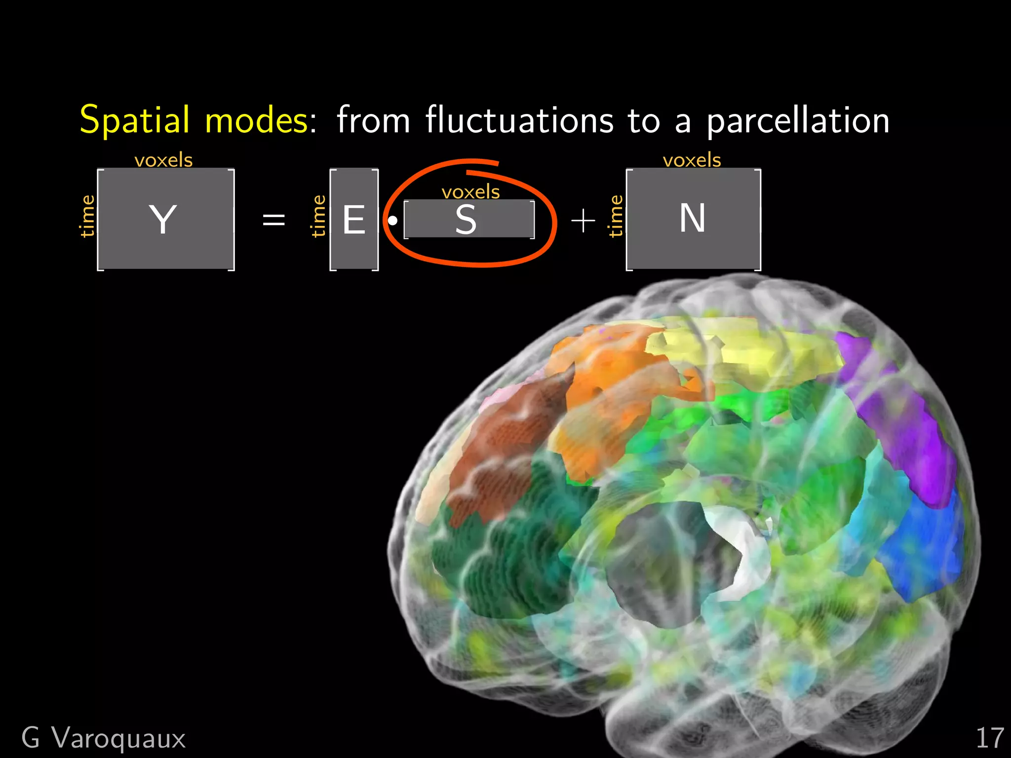
![1 The group-level ICA maps
ICA extracts a brain parcellation
However
No overall control of residuals
Does not select for what we interpret
G Varoquaux [Varoquaux NeuroImage 2010] 12](https://image.slidesharecdn.com/slides-110908185048-phpapp02/75/Learning-and-comparing-multi-subject-models-of-brain-functional-connecitivity-19-2048.jpg)
![1 Multi-subject dictionary learning
Subject Group
Time series maps maps
25 x
Subject level spatial patterns:
Ys = Us Vs T + Es , Es ∼ N (0, σI)
Group level spatial patterns:
Vs = V + Fs , Fs ∼ N (0, ζI)
Sparsity and spatial-smoothness prior:
1
V ∼ exp (−ξ Ω(V)), Ω(v) = v 1 + vT Lv
2
G Varoquaux [Varoquaux Inf Proc Med Imag 2011] 13](https://image.slidesharecdn.com/slides-110908185048-phpapp02/75/Learning-and-comparing-multi-subject-models-of-brain-functional-connecitivity-20-2048.jpg)
![1 Multi-subject dictionary learning
Estimation: maximum a posteriori
argmin Ys − Us Vs T 2
Fro + µ Vs − V 2
Fro + λ Ω(V)
Us ,Vs ,V sujets
Data fit Subject Penalization: sparse
variability and smooth maps
Alternate optimization on Us , Vs , V:
Update Us : standard dictionary learning procedure
[Mairal2010]
Update Vs : ridge regression on (Vs − V)T
Update V: proximal operator for λ Ω:
S
1 s
argmin v −v 2
2 + γ Ω(v) = prox ¯,
v V = mean Vs
¯
v s=1 2
γ/
S Ω s
G Varoquaux [Varoquaux Inf Proc Med Imag 2011] 14](https://image.slidesharecdn.com/slides-110908185048-phpapp02/75/Learning-and-comparing-multi-subject-models-of-brain-functional-connecitivity-21-2048.jpg)
![1 Multi-subject dictionary learning
Estimation: maximum a posteriori
argmin Ys − Us Vs T 2
Fro + µ Vs − V 2
Fro + λ Ω(V)
Us ,Vs ,V sujets
Data fit Subject Penalization: sparse
variability and smooth maps
Parameter selection
µ: comparing variance (PCA spectrum) at subject
and group level
λ: cross-validation
G Varoquaux [Varoquaux Inf Proc Med Imag 2011] 14](https://image.slidesharecdn.com/slides-110908185048-phpapp02/75/Learning-and-comparing-multi-subject-models-of-brain-functional-connecitivity-22-2048.jpg)
![1 Multi-subject dictionary learning
Individual maps + Atlas of functional regions
G Varoquaux [Varoquaux Inf Proc Med Imag 2011] 15](https://image.slidesharecdn.com/slides-110908185048-phpapp02/75/Learning-and-comparing-multi-subject-models-of-brain-functional-connecitivity-23-2048.jpg)
![1 Multi-subject dictionary learning
Multi-subject dictionary learning ICA
G Varoquaux [Varoquaux Inf Proc Med Imag 2011] 16](https://image.slidesharecdn.com/slides-110908185048-phpapp02/75/Learning-and-comparing-multi-subject-models-of-brain-functional-connecitivity-24-2048.jpg)
![1 Multi-subject dictionary learning
Multi-subject dictionary learning ICA
G Varoquaux [Varoquaux Inf Proc Med Imag 2011] 16](https://image.slidesharecdn.com/slides-110908185048-phpapp02/75/Learning-and-comparing-multi-subject-models-of-brain-functional-connecitivity-25-2048.jpg)
![1 Multi-subject dictionary learning
Default mode Base ganglia
G Varoquaux [Varoquaux Inf Proc Med Imag 2011] 16](https://image.slidesharecdn.com/slides-110908185048-phpapp02/75/Learning-and-comparing-multi-subject-models-of-brain-functional-connecitivity-26-2048.jpg)

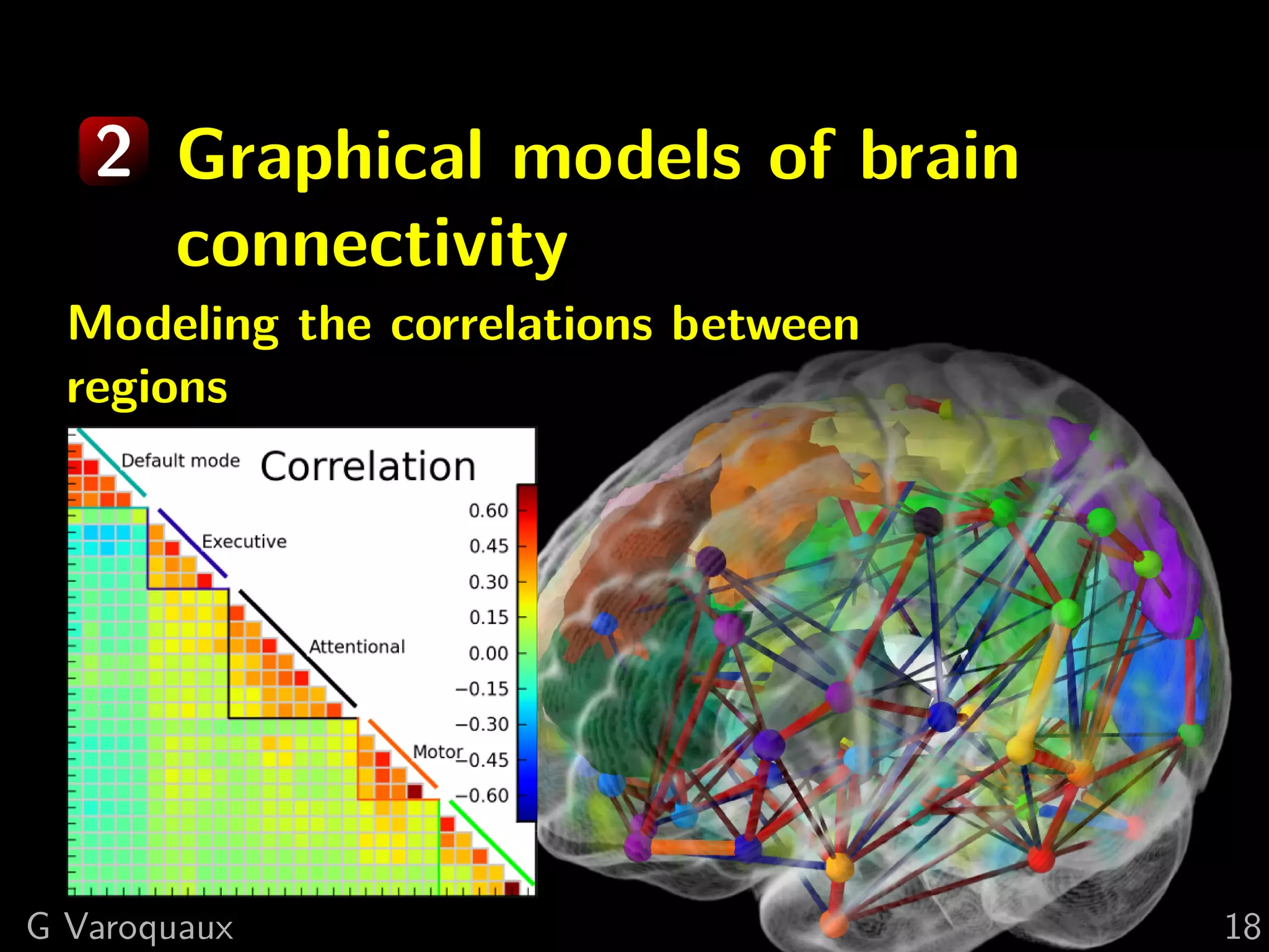
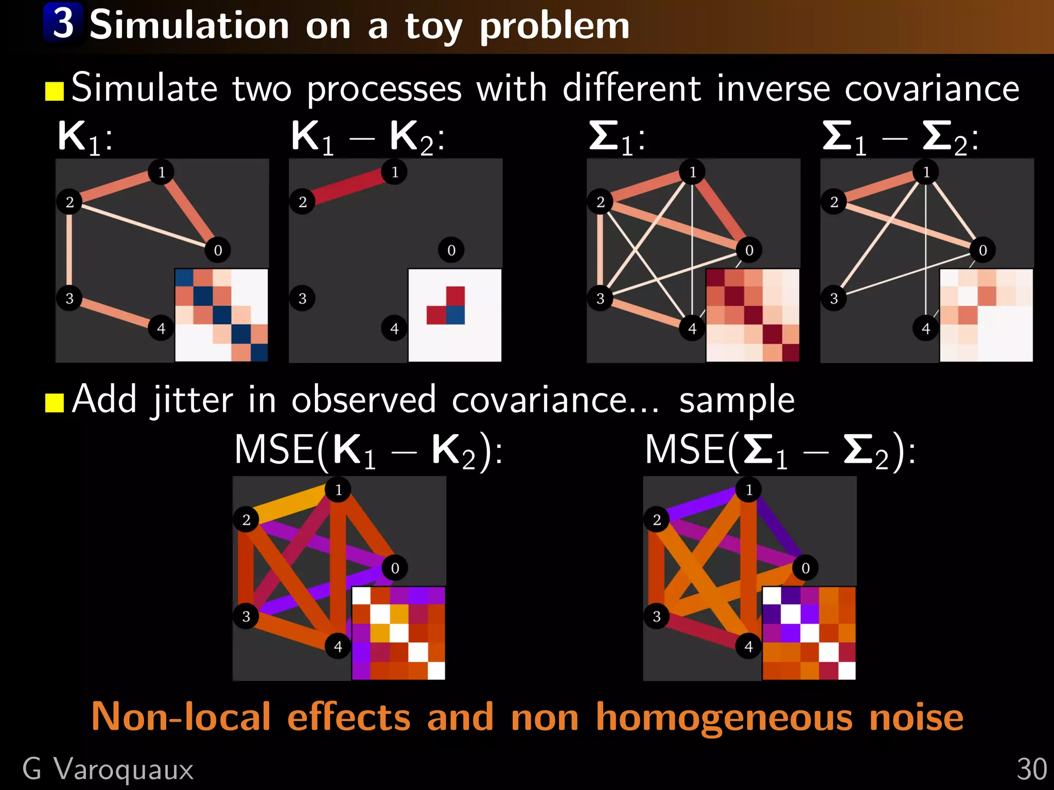
![2 Graphical model for correlation
Specify the probability of observing fMRI data
Multivariate normal P(X) ∝ |Σ−1 |e − 2 X Σ X
1 T −1
Parametrized by inverse covariance matrix K = Σ−1
Observations: Direct connections:
Covariance matrix Inverse covariance
1 1
2 2
0 0
3 3
4 4
[Smith 2011, Varoquaux NIPS 2010]
G Varoquaux 19](https://image.slidesharecdn.com/slides-110908185048-phpapp02/75/Learning-and-comparing-multi-subject-models-of-brain-functional-connecitivity-30-2048.jpg)
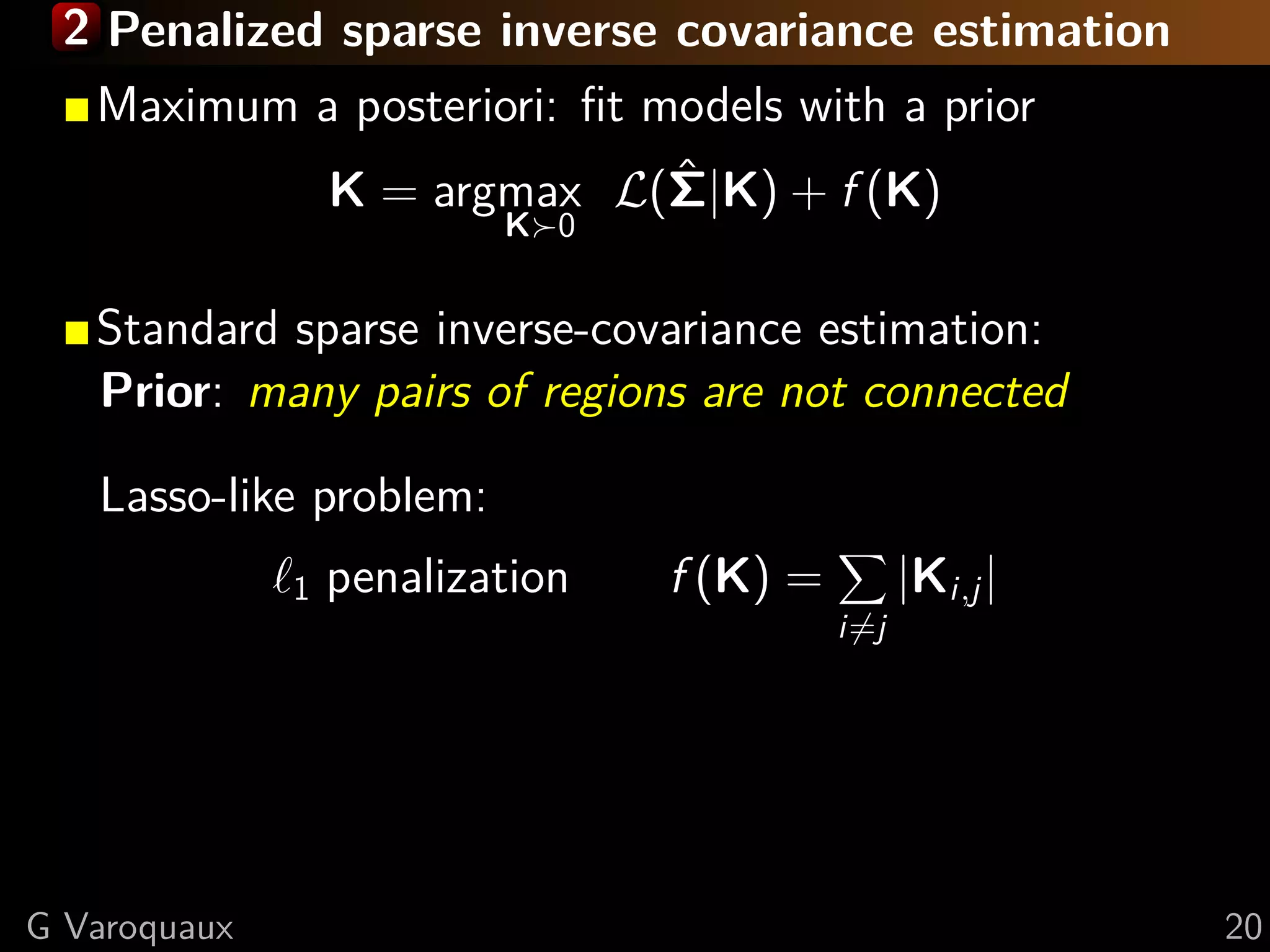
![2 Penalized sparse inverse covariance estimation
Maximum a posteriori: fit models with a prior
K = argmax L(Σ|K) + f (K)
ˆ
K 0
Our contribution: Population prior:
same independence structure across subjects
⇒ Estimate together all {Ks } from {Σs }
ˆ
A. Gramfort
Group-lasso (mixed norms):
21 penalization f {Ks } = λ (Ks )2
i,j
i=j s
Convex optimization problem
G Varoquaux [Varoquaux NIPS 2010] 20](https://image.slidesharecdn.com/slides-110908185048-phpapp02/75/Learning-and-comparing-multi-subject-models-of-brain-functional-connecitivity-32-2048.jpg)
![2 Population-sparse graph perform better
ˆ
Σ−1
Sparse
inverse
Population
prior
Likelihood of new data (nested cross-validation)
Subject data, Σ−1 -57.1
Subject data, sparse inverse 43.0
Group average data, Σ−1 40.6
Group average data, sparse inverse 41.8
Population prior 45.6
G Varoquaux [Varoquaux NIPS 2010] 21](https://image.slidesharecdn.com/slides-110908185048-phpapp02/75/Learning-and-comparing-multi-subject-models-of-brain-functional-connecitivity-33-2048.jpg)
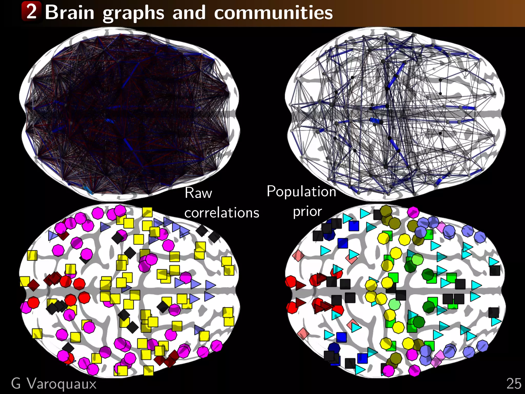
![2 Brain graphs
Raw Population
correlations prior
G Varoquaux [Varoquaux NIPS 2010] 22](https://image.slidesharecdn.com/slides-110908185048-phpapp02/75/Learning-and-comparing-multi-subject-models-of-brain-functional-connecitivity-34-2048.jpg)
![2 Graphs of brain function?
Cognitive function arises from the interplay of
specialized brain regions:
The functional segregation of local areas [...]
contrasts sharply with their global integration during
perception and behavior [Tononi 1994]
A proposed measure of functional segregation
Graph modularity =
divide in communities to
maximize intra-class connections
versus extra-class
G Varoquaux 23](https://image.slidesharecdn.com/slides-110908185048-phpapp02/75/Learning-and-comparing-multi-subject-models-of-brain-functional-connecitivity-35-2048.jpg)
![2 Graph cuts to isolate functional communities
Find communities to maximize modularity:
2
k A(Vc , Vc ) A(V , Vc )
Q= −
c=1 A(V , V ) A(V , V )
A(Va , Vb ) is the sum of edges going from Va to Vb
Rewrite as an eigenvalue problem [White 2005]
1
1
0
0
A · 1 1 0 0
⇒ Spectral clustering = spectral embedding + k-means
Similar to normalized graph cuts
G Varoquaux 24](https://image.slidesharecdn.com/slides-110908185048-phpapp02/75/Learning-and-comparing-multi-subject-models-of-brain-functional-connecitivity-36-2048.jpg)
![2 Brain integration between communities
Proposed measure for functional integration:
mutual information (Tononi)
1
Integration: Ic1 = log det(Kc1 )
2
Mutual information: Mc1 ,c2 = Ic1 ∪c2 − Ic1 − Is2
G Varoquaux [Varoquaux NIPS 2010] 26](https://image.slidesharecdn.com/slides-110908185048-phpapp02/75/Learning-and-comparing-multi-subject-models-of-brain-functional-connecitivity-38-2048.jpg)
![2 Brain integration between communities
Proposed measure for functional integration:
mutual information (Tononi)
With population prior: Occipital pole
Default mode network visual areas Medial visual areas
Fronto-parietal Lateral visual
networks areas
Fronto-lateral Posterior inferior
network temporal 1
Pars Posterior inferior
opercularis temporal 2
Raw Dorsal motor Right Thalamus
correlations: Cingulo-insular
Ventral motor network
Auditory Left Putamen
Basal ganglia
G Varoquaux [Varoquaux NIPS 2010] 26](https://image.slidesharecdn.com/slides-110908185048-phpapp02/75/Learning-and-comparing-multi-subject-models-of-brain-functional-connecitivity-39-2048.jpg)
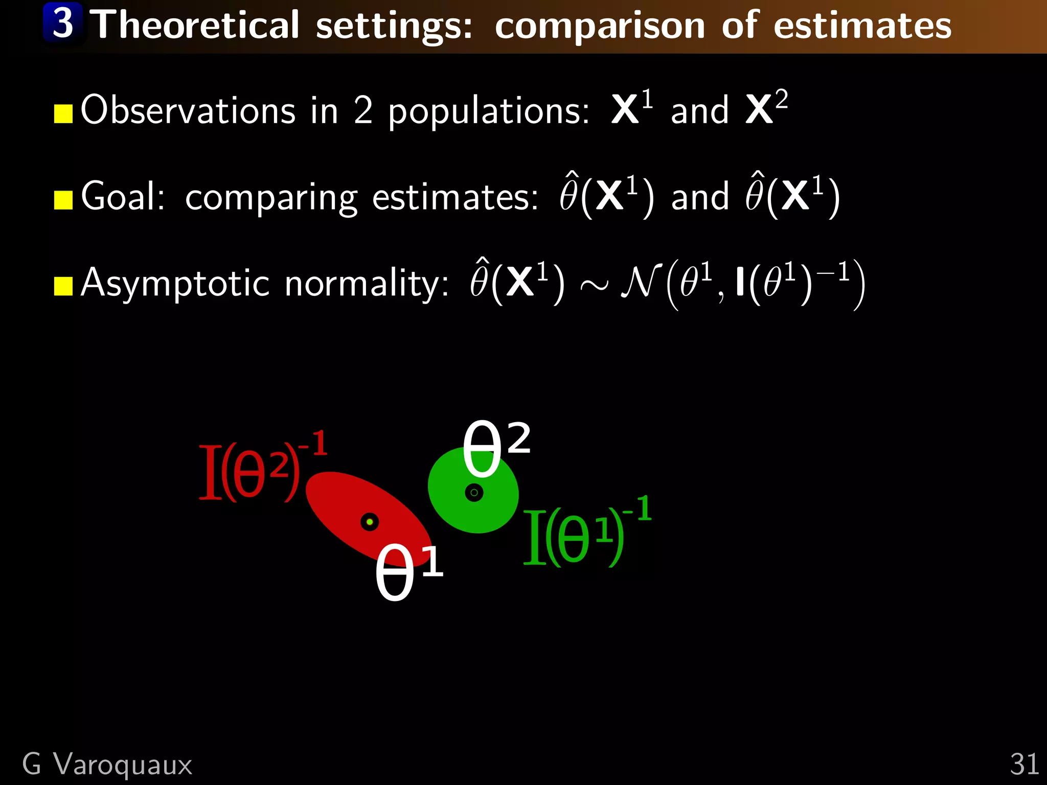
![3 Theoretical settings: comparison of estimates
[Rao 1945] Fisher information I defines a metric on
the manifold of models.
We use it to choose a global parametrization for
comparisons
if old
an
M
G Varoquaux 31](https://image.slidesharecdn.com/slides-110908185048-phpapp02/75/Learning-and-comparing-multi-subject-models-of-brain-functional-connecitivity-47-2048.jpg)
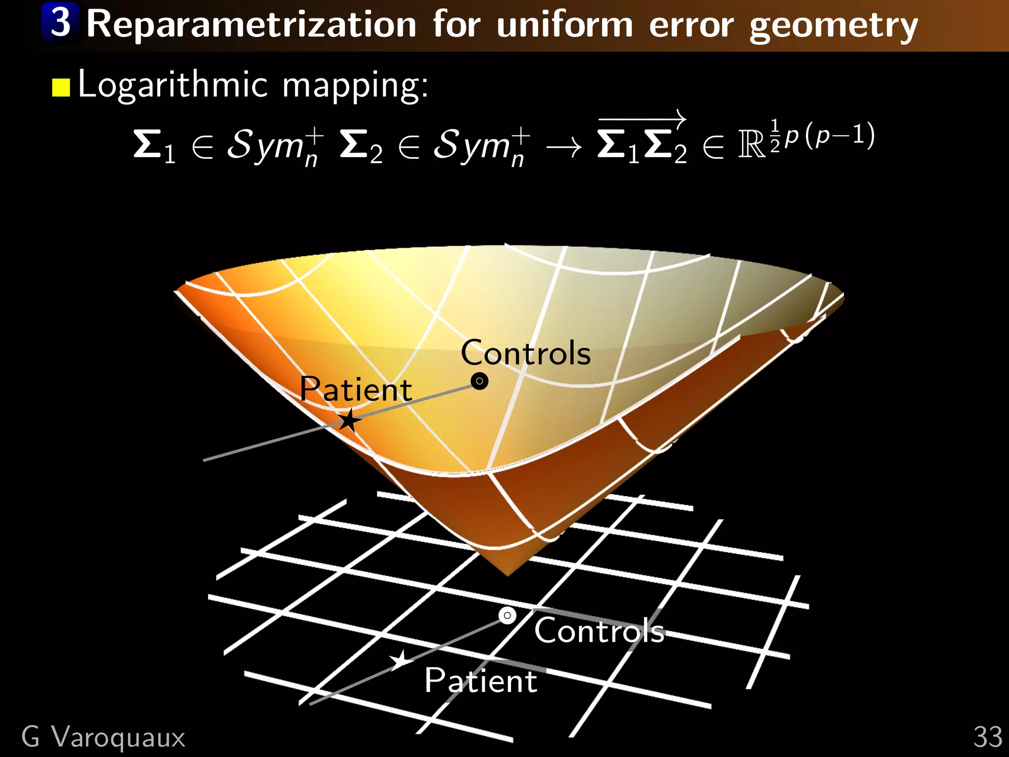
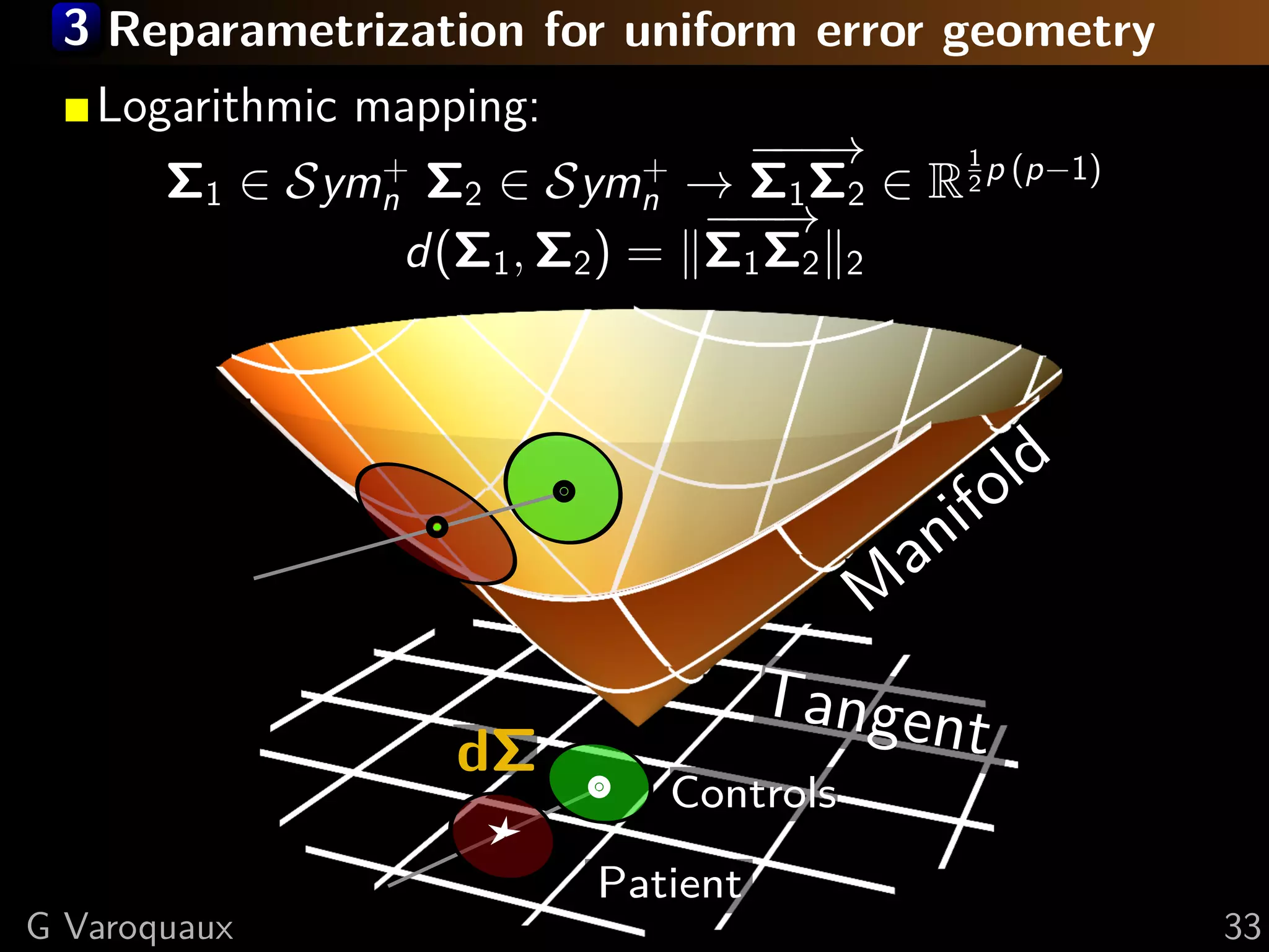
![3 Covariance manifold – Symn
+
Metric tensor (Fisher information) [Lenglet 2006]
dΣ1 , dΣ2 Σ = 1 trace(Σ−1 dΣ1 Σ−1 dΣ2 )
2
+
Nice properties of the Symn manifold (Lie group):
metric can be fully integrated, gives rise to global
mapping to a vector space (Logarithmic map).
Σ1 , Σ2 = log Σ1 − 2 Σ2 Σ1 − 2
2 1 1 2
Σ1
,
Locally: Σ1 , Σ2 ∝ trace(Σ1 − 2 Σ2 Σ1 − 2 ) − p
1 1
Σ1
= dΣ Fro
dΣ = Σ1 Σ2 Σ1
−1/2 −1/2
where
G Varoquaux 32](https://image.slidesharecdn.com/slides-110908185048-phpapp02/75/Learning-and-comparing-multi-subject-models-of-brain-functional-connecitivity-48-2048.jpg)
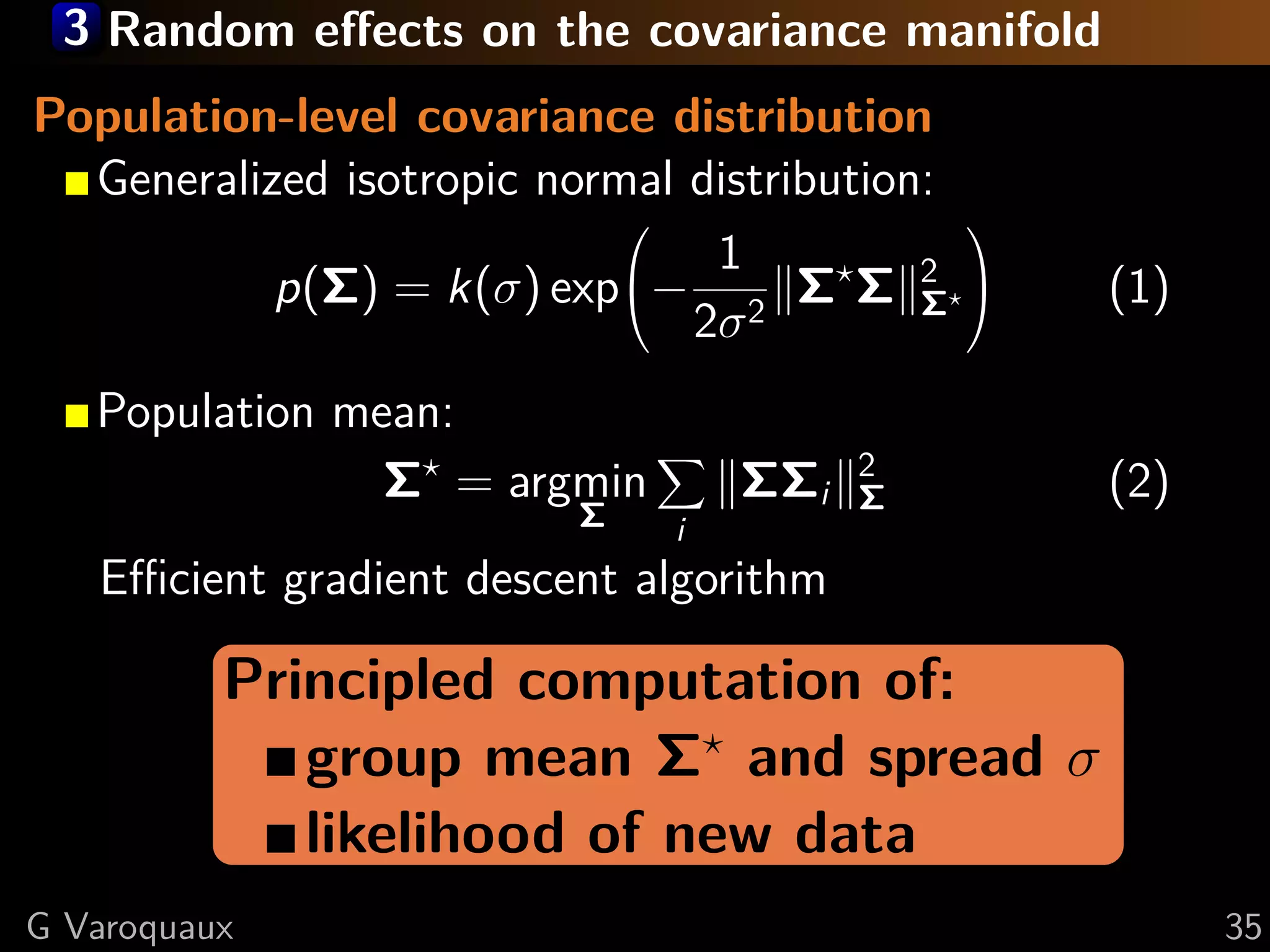
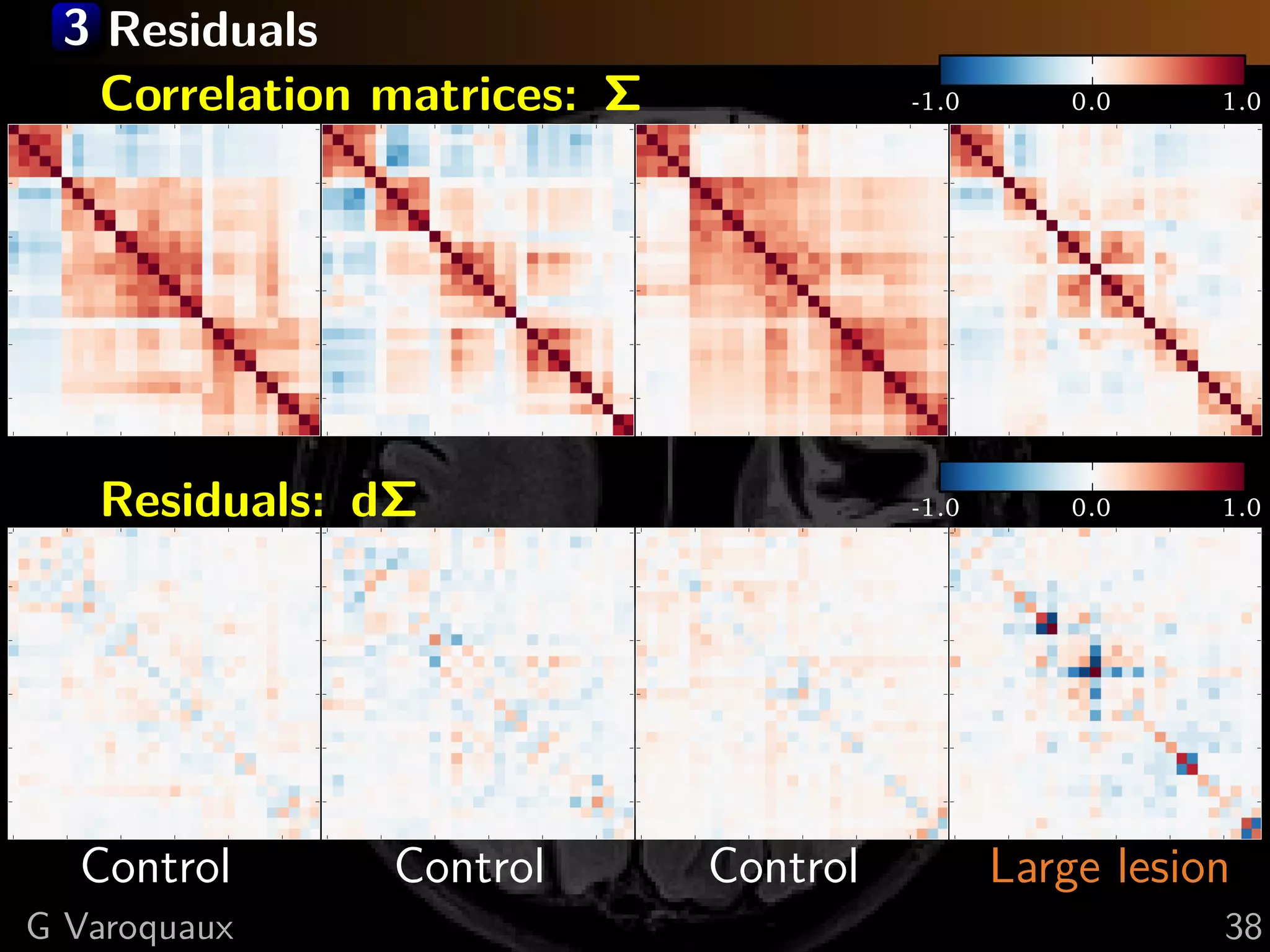
![3 Random effects on the covariance manifold
Population-level covariance distribution
Generalized isotropic normal distribution:
1
p(Σ) = k(σ) exp− 2 Σ Σ 2 Σ
(1)
2σ
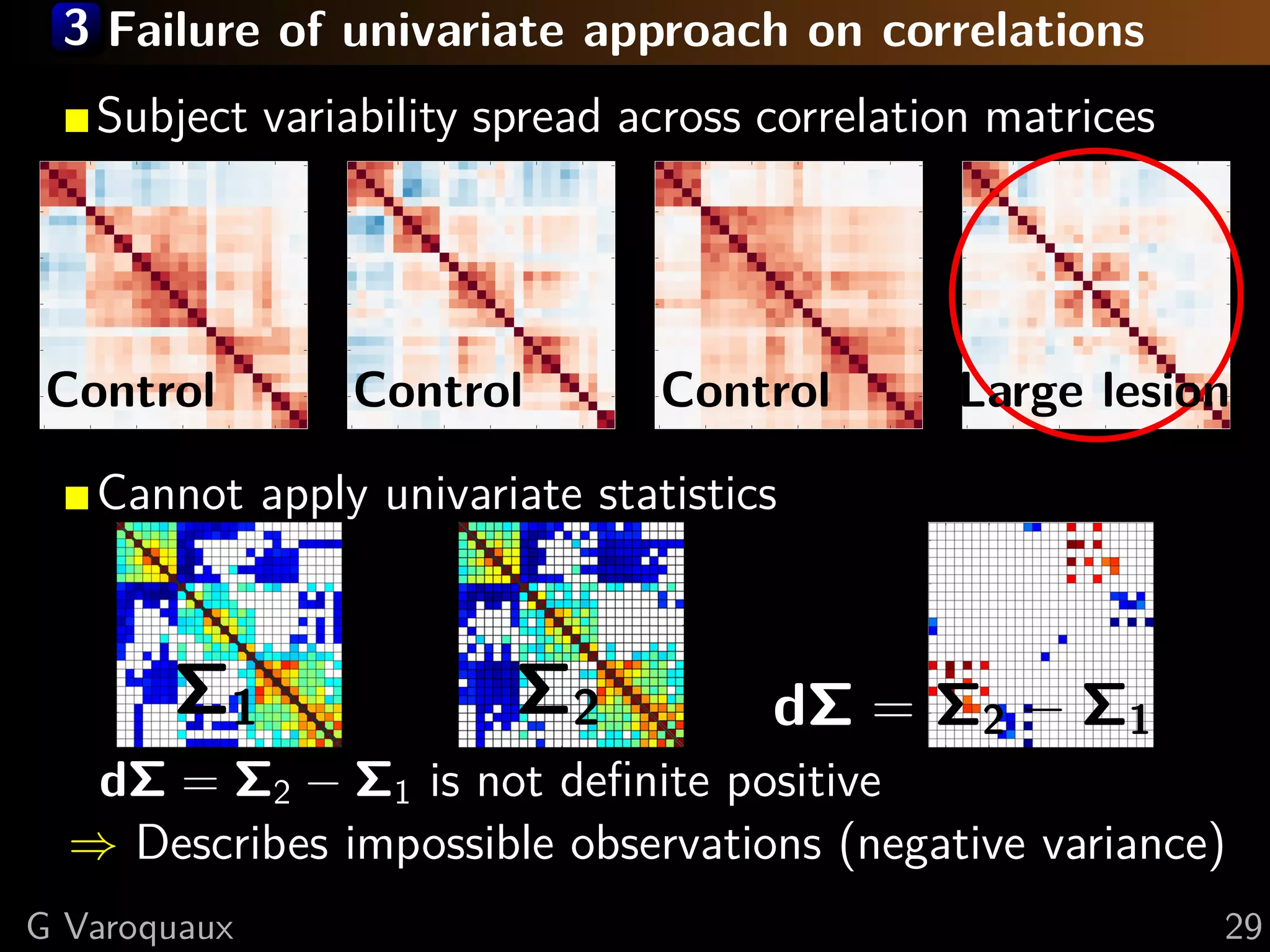
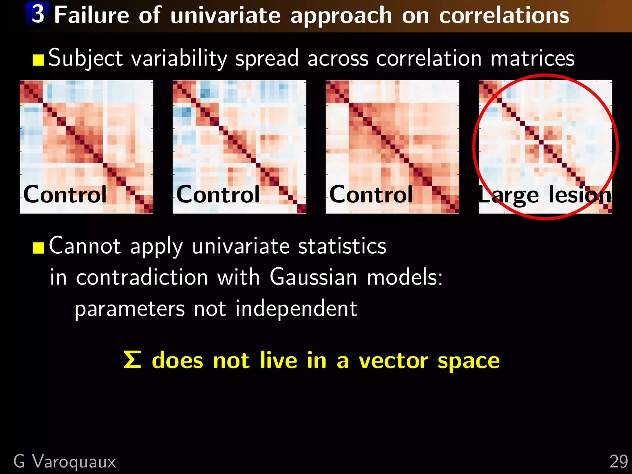
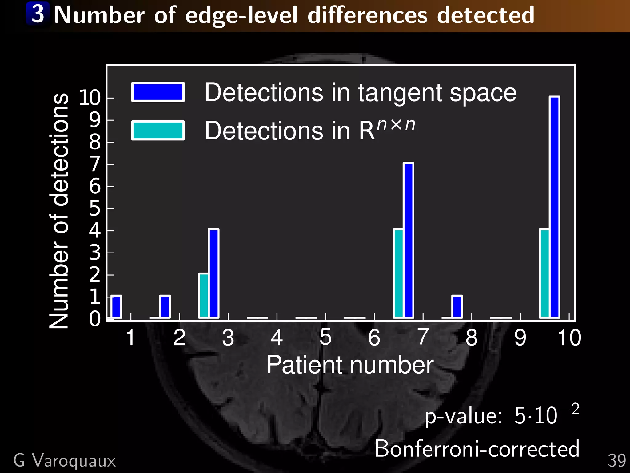
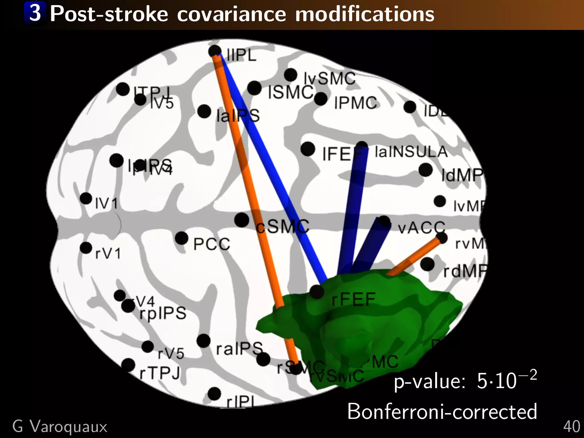
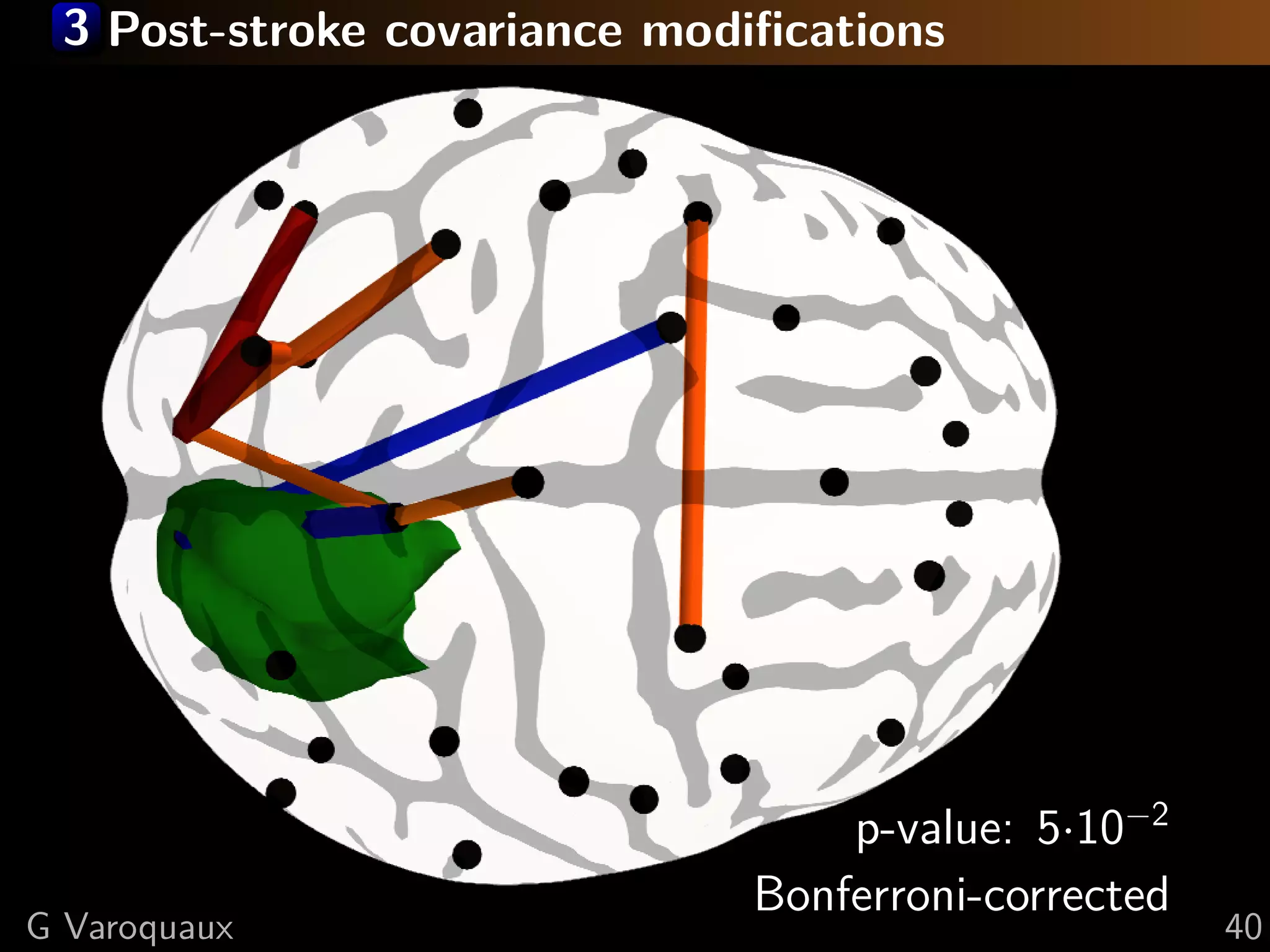
Edge-level statistics
Under null hypothesis: subject ∈ group model (1)
−→
dΣ ∼ N (0, σI) : Independant coefficients
⇒ Univariate statistics on dΣi,j
[Varoquaux MICCAI 2010]
G Varoquaux 35](https://image.slidesharecdn.com/slides-110908185048-phpapp02/75/Learning-and-comparing-multi-subject-models-of-brain-functional-connecitivity-53-2048.jpg)
![Bibliography
[Varoquaux NeuroImage 2010] G. Varoquaux, S. Sadaghiani, P. Pinel, A.
Kleinschmidt, J.B. Poline, B. Thirion A group model for stable multi-subject ICA
on fMRI datasets, NeuroImage 51 p. 288 (2010)
http://hal.inria.fr/hal-00489507/en
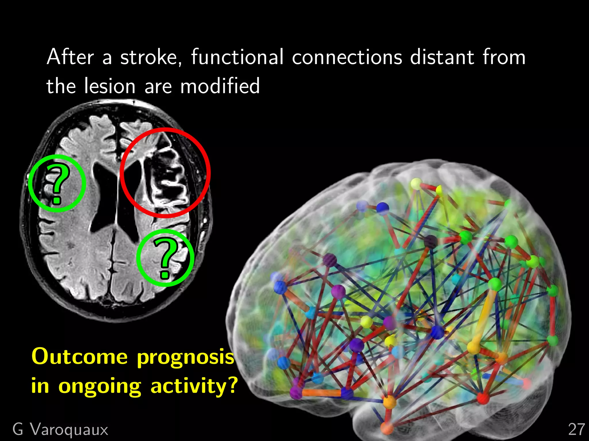
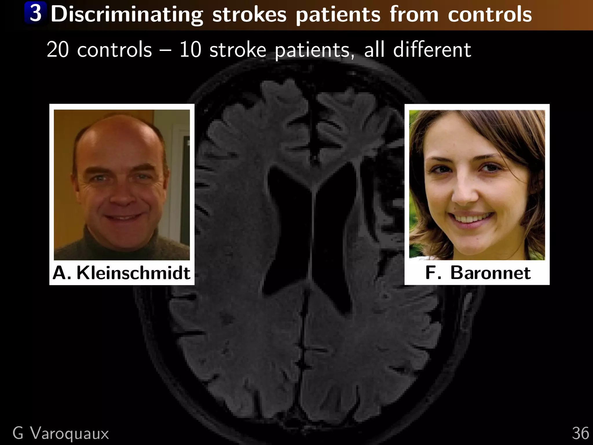
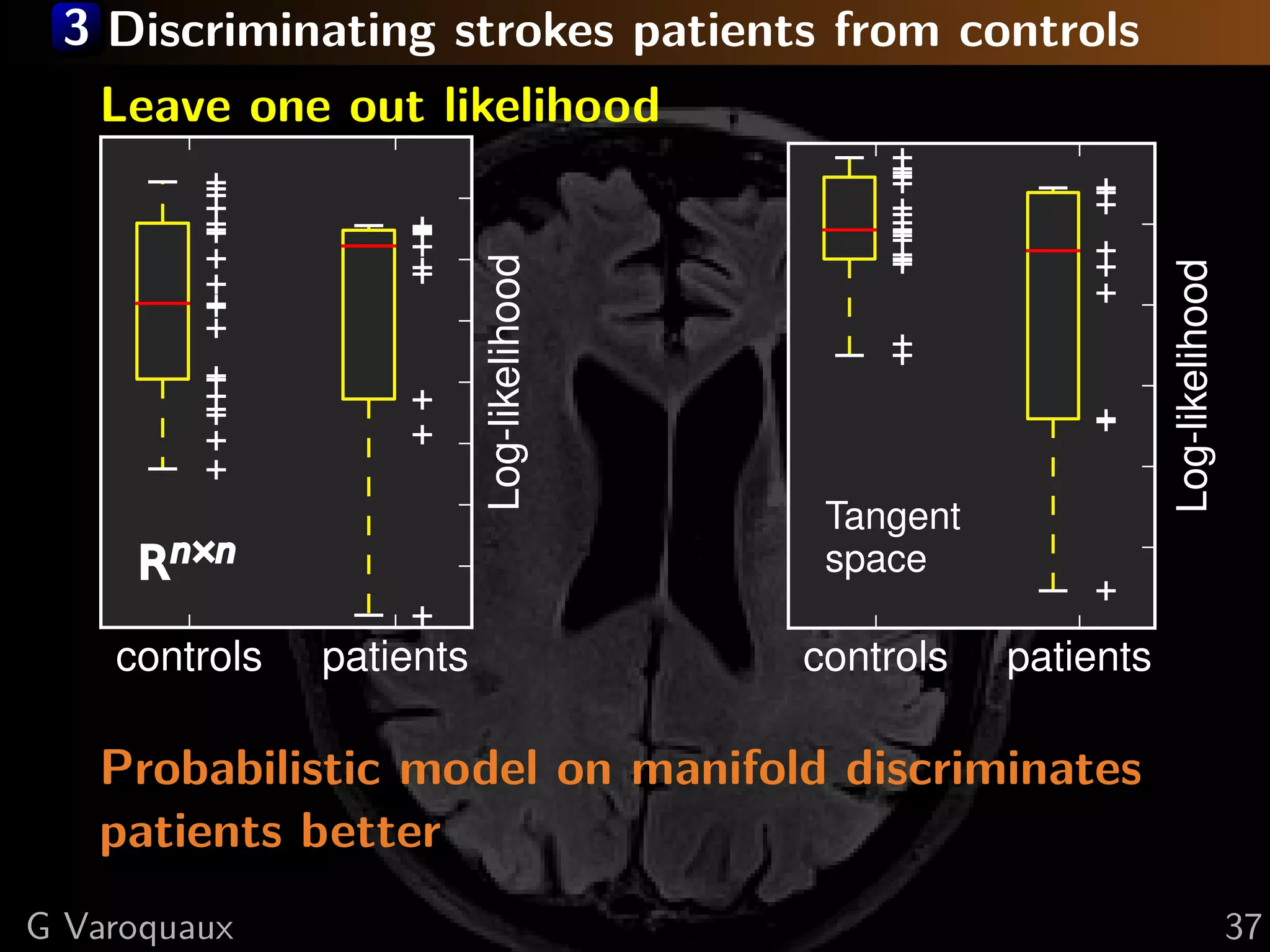
[Varoquaux MICCAI 2010] G. Varoquaux, F. Baronnet, A. Kleinschmidt, P.
Fillard and B. Thirion, Detection of brain functional-connectivity difference in
post-stroke patients using group-level covariance modeling, MICCAI (2010)
http://hal.inria.fr/inria-00512417/en
[Varoquaux NIPS 2010] G. Varoquaux, A. Gramfort, J.B. Poline and B. Thirion,
Brain covariance selection: better individual functional connectivity models using
population prior, NIPS (2010)
http://hal.inria.fr/inria-00512451/en
[Varoquaux IPMI 2011] G. Varoquaux, A. Gramfort, F. Pedregosa, V. Michel,
and B. Thirion, Multi-subject dictionary learning to segment an atlas of brain
spontaneous activity, Information Processing in Medical Imaging p. 562 (2011)
http://hal.inria.fr/inria-00588898/en
[Ramachandran 2011] P. Ramachandran, G. Varoquaux Mayavi: 3d visualization
of scientific data, Computing in Science & Engineering 13 p. 40 (2011)
http://hal.inria.fr/inria-00528985/en
G Varoquaux 43](https://image.slidesharecdn.com/slides-110908185048-phpapp02/75/Learning-and-comparing-multi-subject-models-of-brain-functional-connecitivity-62-2048.jpg)

The document discusses multi-subject models of brain functional connectivity, including the use of statistical and generative models to account for subject variability in neuroimaging data. It explores methods such as Independent Component Analysis (ICA), multi-subject dictionary learning, and graphical models for analyzing brain connectivity and detecting differences in connectivity across groups. Additionally, it emphasizes the need for population-level models and proper statistical methods to improve diagnostic markers and understanding of brain function in various conditions.


![[Harvard CS264] 13 - The R-Stream High-Level Program Transformation Tool / Pr...](https://cdn.slidesharecdn.com/ss_thumbnails/reservoirlabsharvard-presentation-110412184012-phpapp02-thumbnail.jpg?width=640&height=640&fit=bounds)


![Vibe Coding vs. Spec-Driven Development [Free Meetup]](https://cdn.slidesharecdn.com/ss_thumbnails/vibecodingvsspecdrivendevelopment-251209105622-43f455e7-thumbnail.jpg?width=640&height=640&fit=bounds)