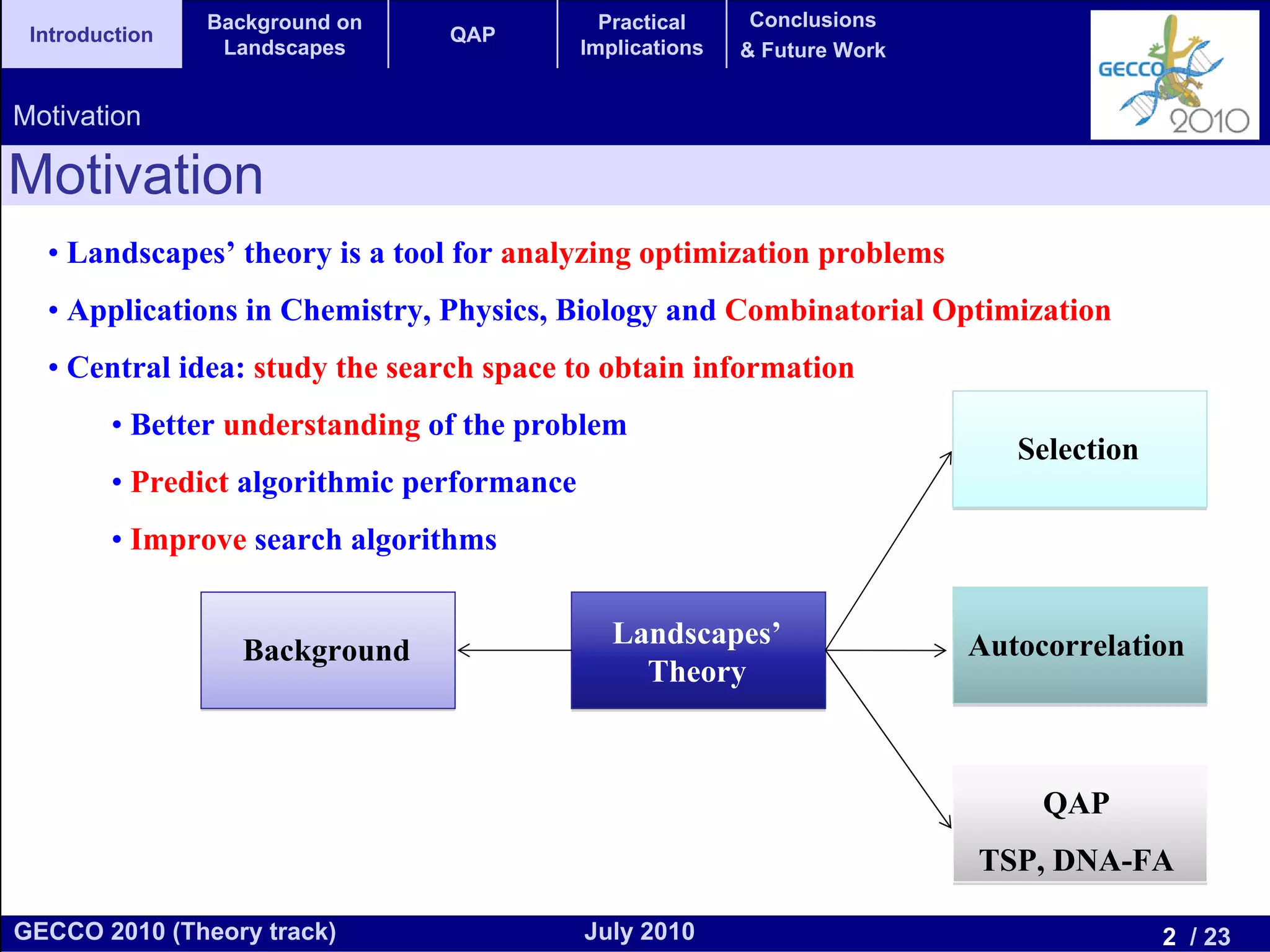
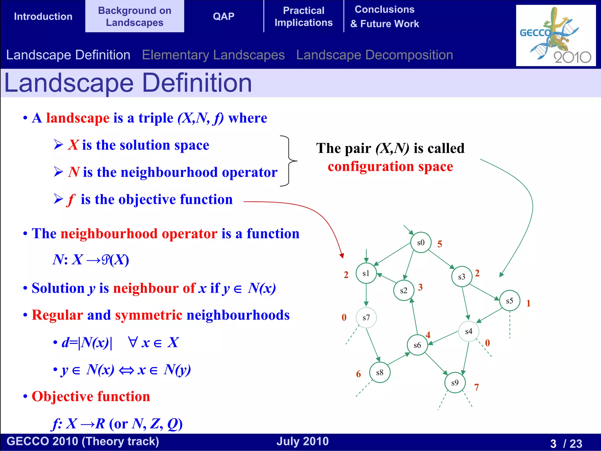
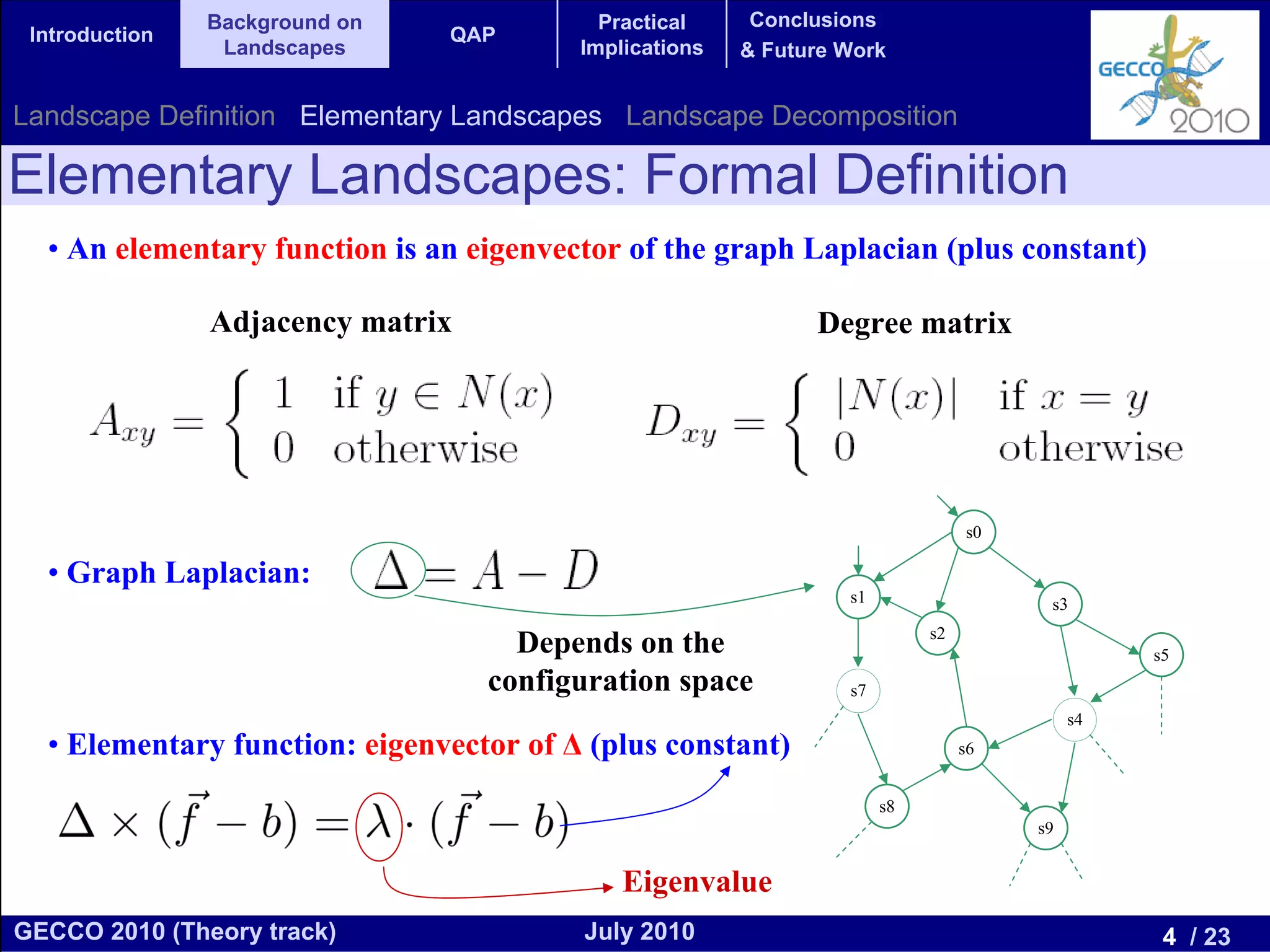
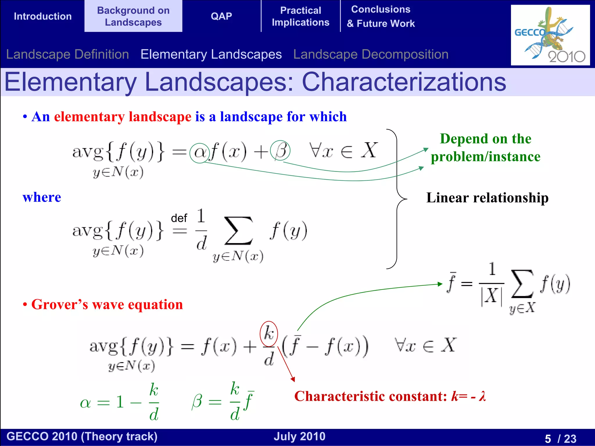
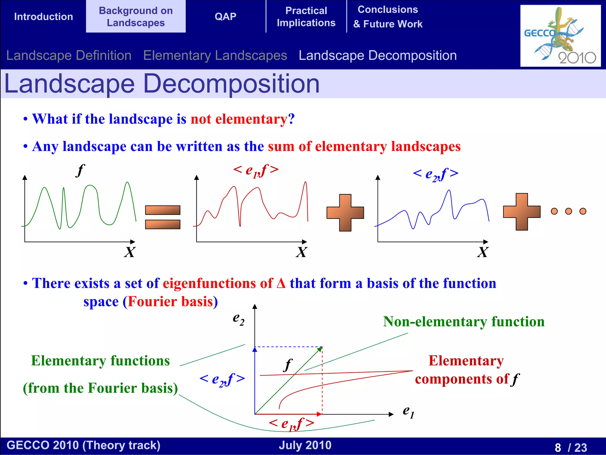
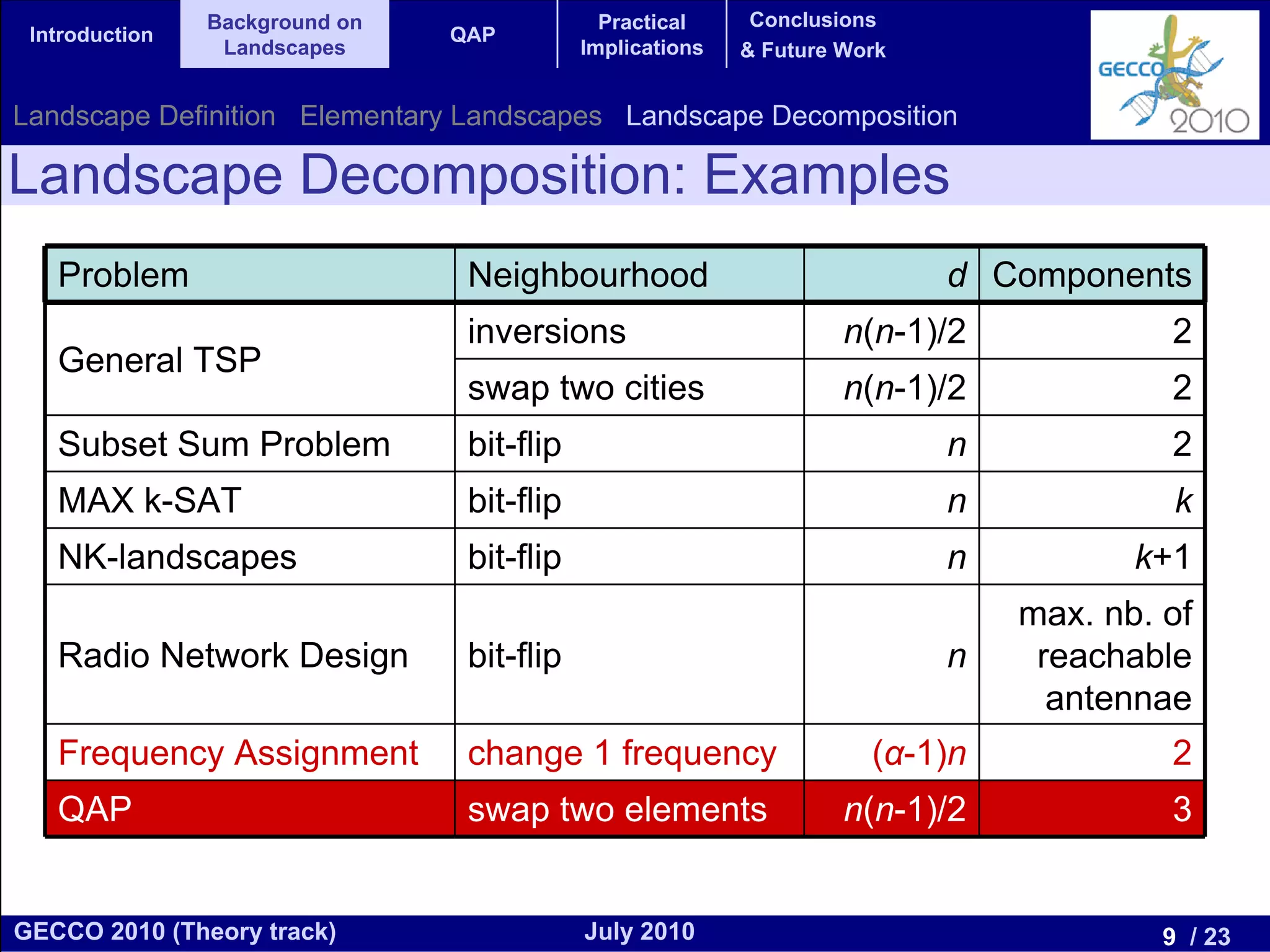
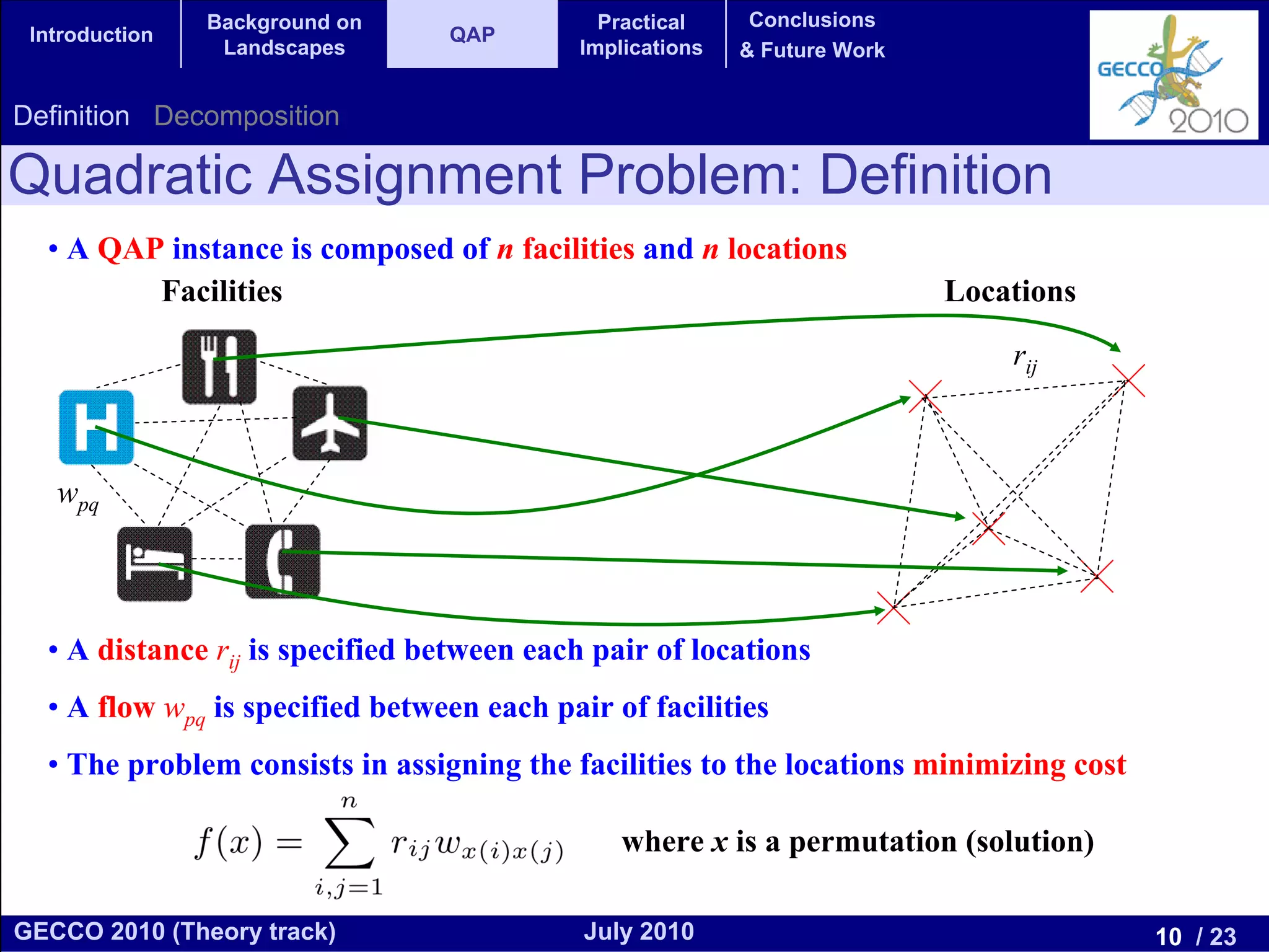
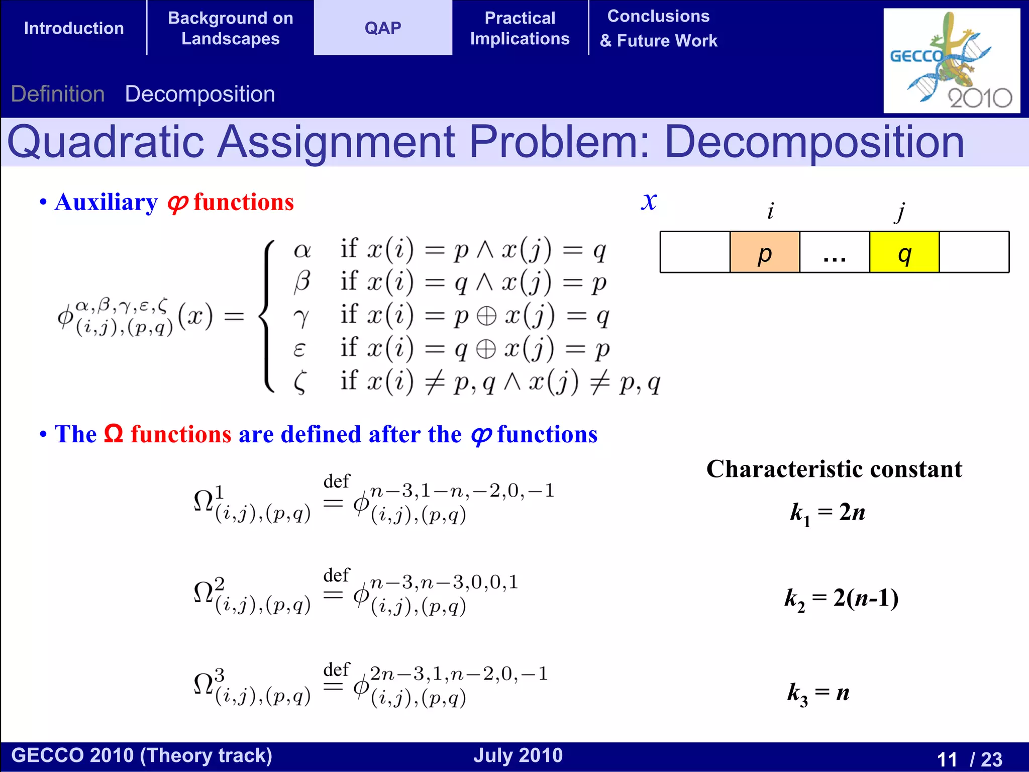
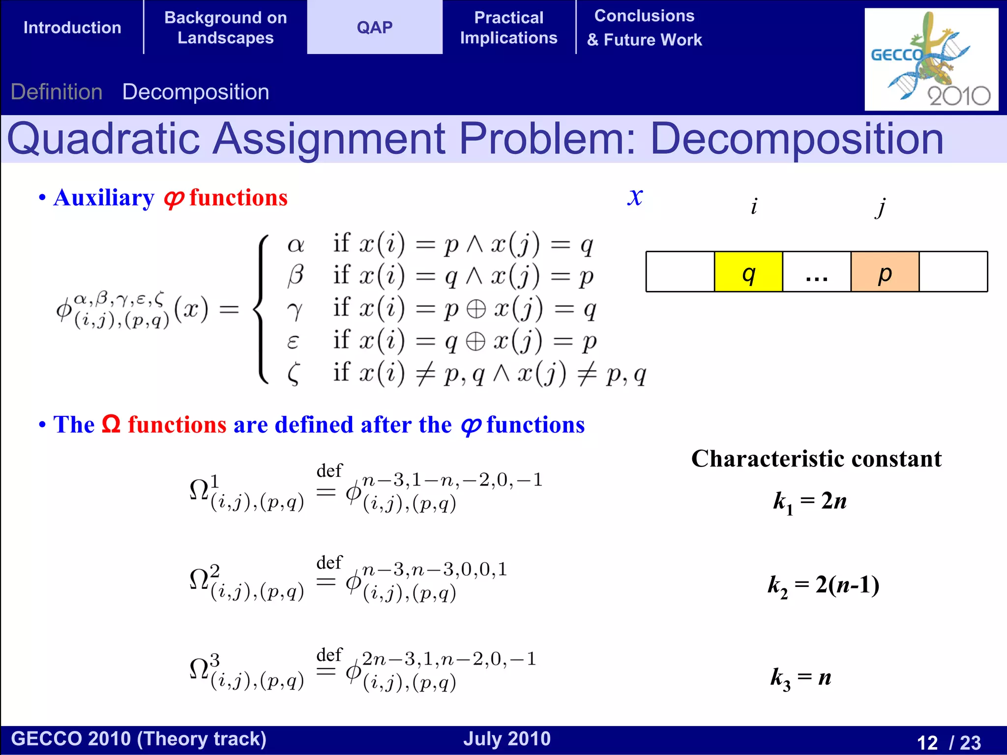
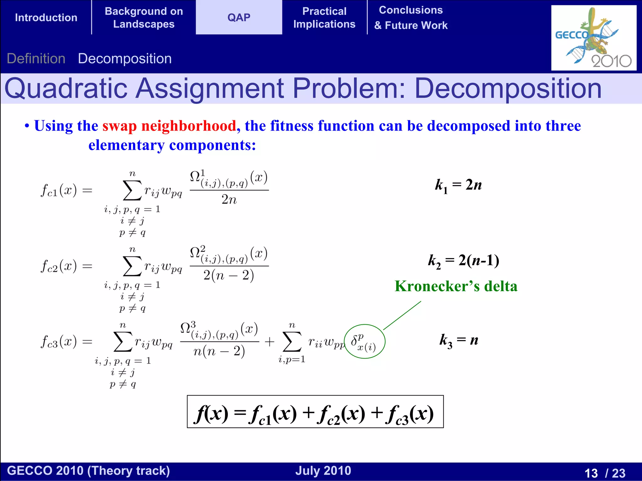
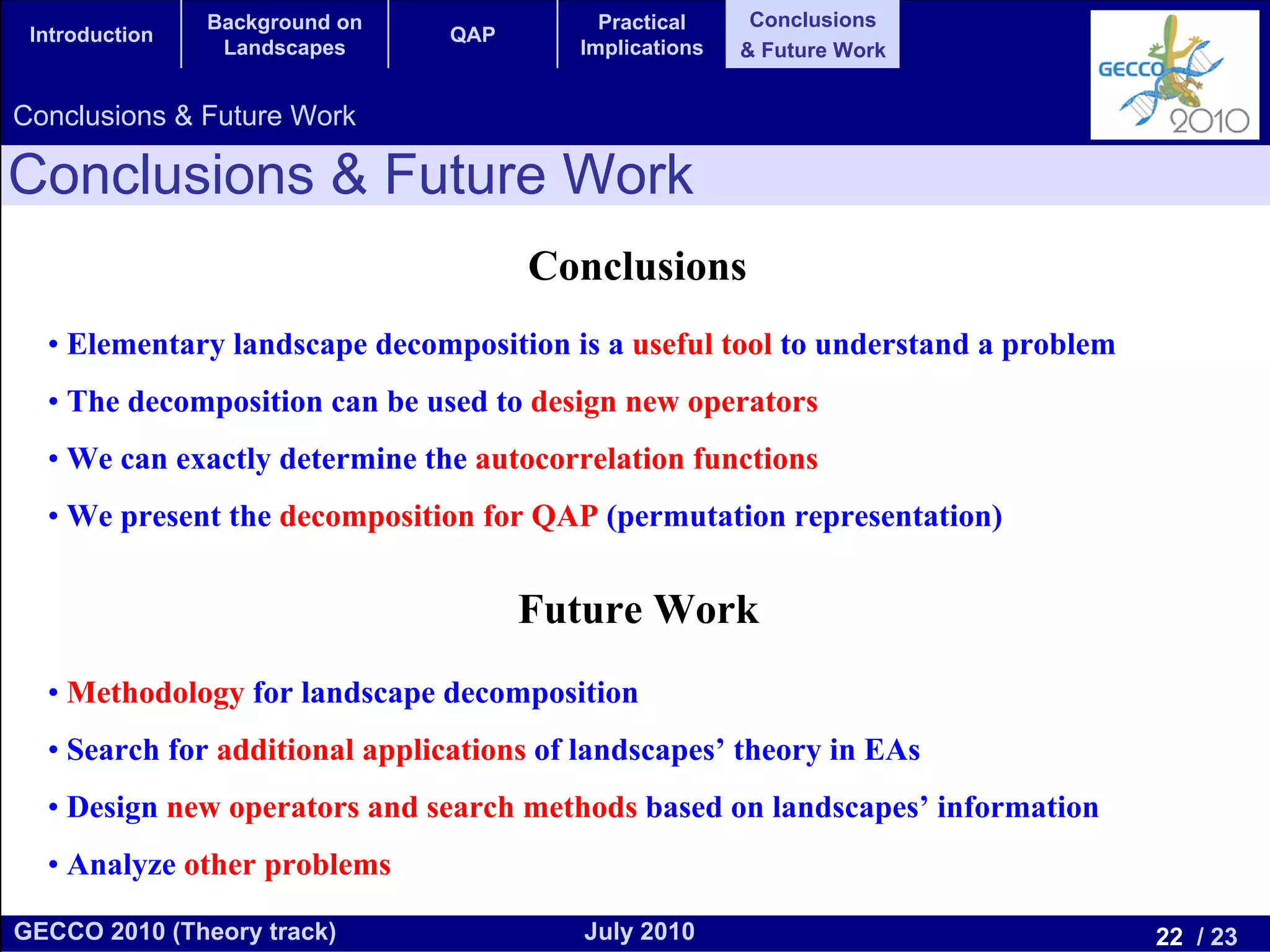
Background on           Practical     Conclusions
 Introduction                   QAP
                 Landscapes           Implications   & Future Work


     Elementary Landscape Decomposition of
        the Quadratic Assignment Problem


    Francisco Chicano, Gabriel Luque, and Enrique Alba


GECCO 2010 (Theory track)             July 2010                      1 / 23
Background on                 Practical     Conclusions
 Introduction                   QAP
                 Landscapes                 Implications   & Future Work


Motivation

Motivation
  • Landscapes’ theory is a tool for analyzing optimization problems
  • Applications in Chemistry, Physics, Biology and Combinatorial Optimization
  • Central idea: study the search space to obtain information
        • Better understanding of the problem
                                                                              Selection
        • Predict algorithmic performance
        • Improve search algorithms

                                               Landscapes’                 Autocorrelation
                  Background
                                                 Theory


                                                                                QAP
                                                                           TSP, DNA-FA

GECCO 2010 (Theory track)                   July 2010                                     2 / 23
Background on                  Practical         Conclusions
 Introduction                         QAP
                 Landscapes                  Implications       & Future Work


Landscape Definition Elementary Landscapes Landscape Decomposition

Landscape Definition
  • A landscape is a triple (X,N, f) where
            X is the solution space                  The pair (X,N) is called
            N is the neighbourhood operator           configuration space

            f is the objective function

  • The neighbourhood operator is a function                                        s0       5
        N: X →P(X)
                                                            2        s1                           s3       2
  • Solution y is neighbour of x if y ∈ N(x)                                   s2    3
                                                                                                                   s5   1
  • Regular and symmetric neighbourhoods                    0        s7
                                                                                                      s4
                                                                                         4
        • d=|N(x)|   ∀x∈X                                                           s6                         0

        • y ∈ N(x) ⇔ x ∈ N(y)                                    6        s8
                                                                                                 s9
                                                                                                           7
  • Objective function
        f: X →R (or N, Z, Q)
GECCO 2010 (Theory track)                      July 2010                                                                    3 / 23
Background on              Practical     Conclusions
 Introduction                   QAP
                 Landscapes              Implications   & Future Work


Landscape Definition Elementary Landscapes Landscape Decomposition

Elementary Landscapes: Formal Definition
  • An elementary function is an eigenvector of the graph Laplacian (plus constant)

                Adjacency matrix                              Degree matrix


                                                                                s0

  • Graph Laplacian:
                                                                 s1                   s3
                                                                           s2
                                     Depends on the                                            s5
                                   configuration space           s7
                                                                                          s4
  • Elementary function: eigenvector of Δ (plus constant)                       s6


                                                                      s8
                                                                                     s9


                                             Eigenvalue
GECCO 2010 (Theory track)                July 2010                                              4 / 23
Background on                 Practical     Conclusions
 Introduction                         QAP
                 Landscapes                 Implications   & Future Work


Landscape Definition Elementary Landscapes Landscape Decomposition

Elementary Landscapes: Characterizations
  • An elementary landscape is a landscape for which
                                                                            Depend on the
                                                                           problem/instance

  where                                                                    Linear relationship
                                def


  • Grover’s wave equation


                                                Characteristic constant: k= - λ

GECCO 2010 (Theory track)                   July 2010                                         5 / 23
Background on              Practical     Conclusions
 Introduction                   QAP
                 Landscapes              Implications   & Future Work


Landscape Definition Elementary Landscapes Landscape Decomposition

Elementary Landscapes: Properties
  • Several properties of elementary landscapes are the following


  where
  • Local maxima and minima
                                          Local maxima


                                             Local minima
                                                                        X
GECCO 2010 (Theory track)                July 2010                          6 / 23
Background on                Practical     Conclusions
 Introduction                   QAP
                 Landscapes                Implications   & Future Work


Landscape Definition Elementary Landscapes Landscape Decomposition

Elementary Landscapes: Examples
      Problem                   Neighbourhood                                 d           k
                                2-opt                               n(n-3)/2           n-1
      Symmetric TSP
                                swap two cities                     n(n-1)/2         2(n-1)
                                inversions                          n(n-1)/2       n(n+1)/2
      Antisymmetric TSP
                                swap two cities                     n(n-1)/2            2n
      Graph α-Coloring          recolor 1 vertex                          (α-1)n        2α
      Graph Matching            swap two elements                   n(n-1)/2         2(n-1)
      Graph Bipartitioning      Johnson graph                               n2/4     2(n-1)
      NEAS                      bit-flip                                      n          4
      Max Cut                   bit-flip                                      n          4
      Weight Partition          bit-flip                                      n          4

GECCO 2010 (Theory track)                  July 2010                                     7 / 23
Background on                 Practical      Conclusions
 Introduction                         QAP
                     Landscapes                 Implications    & Future Work


Landscape Definition Elementary Landscapes Landscape Decomposition

Landscape Decomposition
  • What if the landscape is not elementary?
  • Any landscape can be written as the sum of elementary landscapes
                f                        < e1,f >                          < e2,f >


                        X                                X                             X

  • There exists a set of eigenfunctions of Δ that form a basis of the function
           space (Fourier basis)
                                     e2                     Non-elementary function

    Elementary functions                             f                          Elementary
                                    < e2,f >                                  components of f
  (from the Fourier basis)
                                                                         e1
                                               < e1,f >
GECCO 2010 (Theory track)                           July 2010                                   8 / 23
Background on                 Practical     Conclusions
 Introduction                   QAP
                 Landscapes                 Implications   & Future Work


Landscape Definition Elementary Landscapes Landscape Decomposition

Landscape Decomposition: Examples
   Problem                       Neighbourhood                             d Components
                                 inversions                         n(n-1)/2            2
   General TSP
                                 swap two cities                    n(n-1)/2            2
   Subset Sum Problem            bit-flip                                  n            2
   MAX k-SAT                     bit-flip                                  n             k
   NK-landscapes                 bit-flip                                  n          k+1
                                                                               max. nb. of
   Radio Network Design          bit-flip                                  n    reachable
                                                                                 antennae
   Frequency Assignment          change 1 frequency                   (α-1)n            2
   QAP                           swap two elements                  n(n-1)/2            3


GECCO 2010 (Theory track)                   July 2010                                   9 / 23
Background on                 Practical     Conclusions
 Introduction                    QAP
                 Landscapes                 Implications   & Future Work


Definition Decomposition

Quadratic Assignment Problem: Definition
  • A QAP instance is composed of n facilities and n locations
         Facilities                                                        Locations

                                                                               rij


   wpq


  • A distance rij is specified between each pair of locations
  • A flow wpq is specified between each pair of facilities
  • The problem consists in assigning the facilities to the locations minimizing cost

                                                where x is a permutation (solution)

GECCO 2010 (Theory track)                   July 2010                                   10 / 23
Background on                 Practical     Conclusions
 Introduction                         QAP
                 Landscapes                 Implications   & Future Work


Definition Decomposition

Quadratic Assignment Problem: Decomposition
  • Auxiliary ϕ functions                                      x           i             j
                                                                           p      …      q


  • The Ω functions are defined after the ϕ functions
                                def
                                                                      Characteristic constant
                                                                               k1 = 2n

                                def
                                                                               k2 = 2(n-1)

                                def
                                                                               k3 = n

GECCO 2010 (Theory track)                   July 2010                                        11 / 23
Background on                 Practical     Conclusions
 Introduction                         QAP
                 Landscapes                 Implications   & Future Work


Definition Decomposition

Quadratic Assignment Problem: Decomposition
  • Auxiliary ϕ functions                                      x           i             j

                                                                           q      …      p


  • The Ω functions are defined after the ϕ functions
                                def
                                                                      Characteristic constant
                                                                               k1 = 2n

                                def
                                                                               k2 = 2(n-1)

                                def
                                                                               k3 = n

GECCO 2010 (Theory track)                   July 2010                                        12 / 23
Background on                 Practical     Conclusions
 Introduction                       QAP
                 Landscapes                 Implications   & Future Work


Definition Decomposition

Quadratic Assignment Problem: Decomposition
  • Using the swap neighborhood, the fitness function can be decomposed into three
            elementary components:

                                                                     k1 = 2n


                                                                    k2 = 2(n-1)
                                                              Kronecker’s delta


                                                                      k3 = n


                                f(x) = fc1(x) + fc2(x) + fc3(x)

GECCO 2010 (Theory track)                   July 2010                                13 / 23
Background on                   Practical     Conclusions
 Introduction                       QAP
                 Landscapes                   Implications   & Future Work


Selection Strategy Autocorrelation Subproblems

New Selection Strategy
  • Selection operators usually take into account the fitness value of the individuals

                                Average-based selection
                                                          avg
                                 avg                                              Minimizing


                                                                Fitness-based selection
                                                                        Neighbourhoods

                                                                                    X


  • We can improve the selection operator by selecting the individuals according to
           the average value in their neighbourhoods


GECCO 2010 (Theory track)                     July 2010                                   14 / 23
Background on                Practical     Conclusions
 Introduction                   QAP
                 Landscapes                Implications   & Future Work


Selection Strategy Autocorrelation Subproblems

New Selection Strategy
  • In elementary landscapes the traditional and the new operator are the same!
        Recall that...


  • However, they are not the same in non-elementary landscapes. If we have n
          elementary components, then:


                                                                      Elementary components
  • The new selection strategy could be useful for plateaus
                                                                          Average-based selection
                                      Fitness-based selection
                                                 ?                            Minimizing
                    avg                    avg

                                                                                           X
GECCO 2010 (Theory track)                  July 2010                                           15 / 23
Background on                Practical     Conclusions
 Introduction                       QAP
                    Landscapes                Implications   & Future Work


Selection Strategy Autocorrelation Subproblems

Autocorrelation
  • Let {x0, x1, ...} a simple random walk on the configuration space where xi+1∈N(xi)
  • The random walk induces a time series {f(x0), f(x1), ...} on a landscape.
  • The autocorrelation function is defined as:                                      s0
                                                                                              5


                                                              2                                             2
                                                                      s1                           s3
                                                                                      3
                                                                                s2                                       1
                                                                                                                    s5
                                                              0
  • The autocorrelation length and coefficient:                       s7
                                                                                          4            s4       0
                                                                                     s6

                                                                  6
                                                                           s8
                                                                                                  s9
                                                                                                            7

  • Autocorrelation length conjecture:

                The number of local optima in a search space is roughly                               Solutions
                                                                                                  reached from x0
                                                                                                    after l moves
GECCO 2010 (Theory track)                     July 2010                                                                  16 / 23
Background on                 Practical     Conclusions
 Introduction                      QAP
                 Landscapes                 Implications   & Future Work


Selection Strategy Autocorrelation Subproblems

Autocorrelation Length Conjecture
  • The higher the value of l and ξ the smaller the number of local optima
  • l and ξ is a measure of ruggedness                Angel, Zissimopoulos. Theoretical
                                                     Computer Science 263:159-172 (2001)
   Length
                                     SA (configuration 1)              SA (configuration 2)
 Coefficient      Ruggedness
                                  % rel. error     nb. of steps % rel. error       nb. of steps
                    10 ≤ ζ < 20             0.2            50,500            0.1       101,395
                    20 ≤ ζ < 30             0.3            53,300            0.2       106,890
                    30 ≤ ζ < 40             0.3            58,700            0.2       118,760
                    40 ≤ ζ < 50             0.5            62,700            0.3       126,395
                    50 ≤ ζ < 60             0.7            66,100            0.4       133,055
                    60 ≤ ζ < 70             1.0            75,300            0.6       151,870
                    70 ≤ ζ < 80             1.3            76,800            1.0       155,230
                    80 ≤ ζ < 90             1.9            79,700            1.4       159,840
                   90 ≤ ζ < 100             2.0            82,400            1.8       165,610

GECCO 2010 (Theory track)                    July 2010                                        17 / 23
Background on               Practical      Conclusions
 Introduction                   QAP
                 Landscapes               Implications    & Future Work


Selection Strategy Autocorrelation Subproblems

Autocorrelation and Landscapes
  • If f is a sum of elementary landscapes:      Fourier coefficients


  • Summing all the squared coefficients with the same ki:


  where


GECCO 2010 (Theory track)                     July 2010                   18 / 23
Background on                Practical     Conclusions
 Introduction                   QAP
                 Landscapes                Implications   & Future Work


Selection Strategy Autocorrelation Subproblems

Autocorrelation for QAP
  • Using the landscape decomposition we can compute l and ξ


  • The bounds for these parameters are:


  • We designed an O(n2) algorithm for this computation (optimal complexity)
  • We computed l and ξ for all the instances in the QAPLIB


GECCO 2010 (Theory track)                  July 2010                           19 / 23
Background on                Practical     Conclusions
 Introduction                   QAP
                 Landscapes                Implications   & Future Work


Selection Strategy Autocorrelation Subproblems

Autocorrelation for QAP
  • Using the landscape decomposition we can compute l and ξ


  • The bounds for these parameters are:


  • We designed an O(n2) algorithm for this computation (optimal complexity)
  • We computed l and ξ for all the instances in the QAPLIB


GECCO 2010 (Theory track)                  July 2010                           20 / 23
Background on               Practical     Conclusions
 Introduction                   QAP
                 Landscapes               Implications   & Future Work


Selection Strategy Autocorrelation Subproblems

Subproblems of QAP: TSP and DNA-FA
  • TSP is a particular case of QAP with two elementary components (fc1 and fc2)


  • The autocorrelation parameters are:


  • DNA Fragment Assembly is a technique to reconstruct an original DNA sequence
          a large number of fragments    Alba, Luque, Khuri, CEC 2005:57-65
  • Two fitness functions are possible and both define QAP subproblems


GECCO 2010 (Theory track)                 July 2010                                21 / 23
Background on              Practical     Conclusions
 Introduction                   QAP
                 Landscapes              Implications   & Future Work


Conclusions & Future Work

Conclusions & Future Work
                                      Conclusions
  • Elementary landscape decomposition is a useful tool to understand a problem
  • The decomposition can be used to design new operators
  • We can exactly determine the autocorrelation functions
  • We present the decomposition for QAP (permutation representation)


                                      Future Work
  • Methodology for landscape decomposition
  • Search for additional applications of landscapes’ theory in EAs
  • Design new operators and search methods based on landscapes’ information
  • Analyze other problems

GECCO 2010 (Theory track)                July 2010                                22 / 23
Elementary Landscape Decomposition of
    the Quadratic Assignment Problem
Thanks for your attention !!!


GECCO 2010 (Theory track)   July 2010    23 / 23

Elementary Landscape Decomposition of the Quadratic Assignment Problem

  • 1.
    Background on Practical Conclusions Introduction QAP Landscapes Implications & Future Work Elementary Landscape Decomposition of the Quadratic Assignment Problem Francisco Chicano, Gabriel Luque, and Enrique Alba GECCO 2010 (Theory track) July 2010 1 / 23
  • 2.
    Background on Practical Conclusions Introduction QAP Landscapes Implications & Future Work Motivation Motivation • Landscapes’ theory is a tool for analyzing optimization problems • Applications in Chemistry, Physics, Biology and Combinatorial Optimization • Central idea: study the search space to obtain information • Better understanding of the problem Selection • Predict algorithmic performance • Improve search algorithms Landscapes’ Autocorrelation Background Theory QAP TSP, DNA-FA GECCO 2010 (Theory track) July 2010 2 / 23
  • 3.
    Background on Practical Conclusions Introduction QAP Landscapes Implications & Future Work Landscape Definition Elementary Landscapes Landscape Decomposition Landscape Definition • A landscape is a triple (X,N, f) where X is the solution space The pair (X,N) is called N is the neighbourhood operator configuration space f is the objective function • The neighbourhood operator is a function s0 5 N: X →P(X) 2 s1 s3 2 • Solution y is neighbour of x if y ∈ N(x) s2 3 s5 1 • Regular and symmetric neighbourhoods 0 s7 s4 4 • d=|N(x)| ∀x∈X s6 0 • y ∈ N(x) ⇔ x ∈ N(y) 6 s8 s9 7 • Objective function f: X →R (or N, Z, Q) GECCO 2010 (Theory track) July 2010 3 / 23
  • 4.
    Background on Practical Conclusions Introduction QAP Landscapes Implications & Future Work Landscape Definition Elementary Landscapes Landscape Decomposition Elementary Landscapes: Formal Definition • An elementary function is an eigenvector of the graph Laplacian (plus constant) Adjacency matrix Degree matrix s0 • Graph Laplacian: s1 s3 s2 Depends on the s5 configuration space s7 s4 • Elementary function: eigenvector of Δ (plus constant) s6 s8 s9 Eigenvalue GECCO 2010 (Theory track) July 2010 4 / 23
  • 5.
    Background on Practical Conclusions Introduction QAP Landscapes Implications & Future Work Landscape Definition Elementary Landscapes Landscape Decomposition Elementary Landscapes: Characterizations • An elementary landscape is a landscape for which Depend on the problem/instance where Linear relationship def • Grover’s wave equation Characteristic constant: k= - λ GECCO 2010 (Theory track) July 2010 5 / 23
  • 6.
    Background on Practical Conclusions Introduction QAP Landscapes Implications & Future Work Landscape Definition Elementary Landscapes Landscape Decomposition Elementary Landscapes: Properties • Several properties of elementary landscapes are the following where • Local maxima and minima Local maxima Local minima X GECCO 2010 (Theory track) July 2010 6 / 23
  • 7.
    Background on Practical Conclusions Introduction QAP Landscapes Implications & Future Work Landscape Definition Elementary Landscapes Landscape Decomposition Elementary Landscapes: Examples Problem Neighbourhood d k 2-opt n(n-3)/2 n-1 Symmetric TSP swap two cities n(n-1)/2 2(n-1) inversions n(n-1)/2 n(n+1)/2 Antisymmetric TSP swap two cities n(n-1)/2 2n Graph α-Coloring recolor 1 vertex (α-1)n 2α Graph Matching swap two elements n(n-1)/2 2(n-1) Graph Bipartitioning Johnson graph n2/4 2(n-1) NEAS bit-flip n 4 Max Cut bit-flip n 4 Weight Partition bit-flip n 4 GECCO 2010 (Theory track) July 2010 7 / 23
  • 8.
    Background on Practical Conclusions Introduction QAP Landscapes Implications & Future Work Landscape Definition Elementary Landscapes Landscape Decomposition Landscape Decomposition • What if the landscape is not elementary? • Any landscape can be written as the sum of elementary landscapes f < e1,f > < e2,f > X X X • There exists a set of eigenfunctions of Δ that form a basis of the function space (Fourier basis) e2 Non-elementary function Elementary functions f Elementary < e2,f > components of f (from the Fourier basis) e1 < e1,f > GECCO 2010 (Theory track) July 2010 8 / 23
  • 9.
    Background on Practical Conclusions Introduction QAP Landscapes Implications & Future Work Landscape Definition Elementary Landscapes Landscape Decomposition Landscape Decomposition: Examples Problem Neighbourhood d Components inversions n(n-1)/2 2 General TSP swap two cities n(n-1)/2 2 Subset Sum Problem bit-flip n 2 MAX k-SAT bit-flip n k NK-landscapes bit-flip n k+1 max. nb. of Radio Network Design bit-flip n reachable antennae Frequency Assignment change 1 frequency (α-1)n 2 QAP swap two elements n(n-1)/2 3 GECCO 2010 (Theory track) July 2010 9 / 23
  • 10.
    Background on Practical Conclusions Introduction QAP Landscapes Implications & Future Work Definition Decomposition Quadratic Assignment Problem: Definition • A QAP instance is composed of n facilities and n locations Facilities Locations rij wpq • A distance rij is specified between each pair of locations • A flow wpq is specified between each pair of facilities • The problem consists in assigning the facilities to the locations minimizing cost where x is a permutation (solution) GECCO 2010 (Theory track) July 2010 10 / 23
  • 11.
    Background on Practical Conclusions Introduction QAP Landscapes Implications & Future Work Definition Decomposition Quadratic Assignment Problem: Decomposition • Auxiliary ϕ functions x i j p … q • The Ω functions are defined after the ϕ functions def Characteristic constant k1 = 2n def k2 = 2(n-1) def k3 = n GECCO 2010 (Theory track) July 2010 11 / 23
  • 12.
    Background on Practical Conclusions Introduction QAP Landscapes Implications & Future Work Definition Decomposition Quadratic Assignment Problem: Decomposition • Auxiliary ϕ functions x i j q … p • The Ω functions are defined after the ϕ functions def Characteristic constant k1 = 2n def k2 = 2(n-1) def k3 = n GECCO 2010 (Theory track) July 2010 12 / 23
  • 13.
    Background on Practical Conclusions Introduction QAP Landscapes Implications & Future Work Definition Decomposition Quadratic Assignment Problem: Decomposition • Using the swap neighborhood, the fitness function can be decomposed into three elementary components: k1 = 2n k2 = 2(n-1) Kronecker’s delta k3 = n f(x) = fc1(x) + fc2(x) + fc3(x) GECCO 2010 (Theory track) July 2010 13 / 23
  • 14.
    Background on Practical Conclusions Introduction QAP Landscapes Implications & Future Work Selection Strategy Autocorrelation Subproblems New Selection Strategy • Selection operators usually take into account the fitness value of the individuals Average-based selection avg avg Minimizing Fitness-based selection Neighbourhoods X • We can improve the selection operator by selecting the individuals according to the average value in their neighbourhoods GECCO 2010 (Theory track) July 2010 14 / 23
  • 15.
    Background on Practical Conclusions Introduction QAP Landscapes Implications & Future Work Selection Strategy Autocorrelation Subproblems New Selection Strategy • In elementary landscapes the traditional and the new operator are the same! Recall that... • However, they are not the same in non-elementary landscapes. If we have n elementary components, then: Elementary components • The new selection strategy could be useful for plateaus Average-based selection Fitness-based selection ? Minimizing avg avg X GECCO 2010 (Theory track) July 2010 15 / 23
  • 16.
    Background on Practical Conclusions Introduction QAP Landscapes Implications & Future Work Selection Strategy Autocorrelation Subproblems Autocorrelation • Let {x0, x1, ...} a simple random walk on the configuration space where xi+1∈N(xi) • The random walk induces a time series {f(x0), f(x1), ...} on a landscape. • The autocorrelation function is defined as: s0 5 2 2 s1 s3 3 s2 1 s5 0 • The autocorrelation length and coefficient: s7 4 s4 0 s6 6 s8 s9 7 • Autocorrelation length conjecture: The number of local optima in a search space is roughly Solutions reached from x0 after l moves GECCO 2010 (Theory track) July 2010 16 / 23
  • 17.
    Background on Practical Conclusions Introduction QAP Landscapes Implications & Future Work Selection Strategy Autocorrelation Subproblems Autocorrelation Length Conjecture • The higher the value of l and ξ the smaller the number of local optima • l and ξ is a measure of ruggedness Angel, Zissimopoulos. Theoretical Computer Science 263:159-172 (2001) Length SA (configuration 1) SA (configuration 2) Coefficient Ruggedness % rel. error nb. of steps % rel. error nb. of steps 10 ≤ ζ < 20 0.2 50,500 0.1 101,395 20 ≤ ζ < 30 0.3 53,300 0.2 106,890 30 ≤ ζ < 40 0.3 58,700 0.2 118,760 40 ≤ ζ < 50 0.5 62,700 0.3 126,395 50 ≤ ζ < 60 0.7 66,100 0.4 133,055 60 ≤ ζ < 70 1.0 75,300 0.6 151,870 70 ≤ ζ < 80 1.3 76,800 1.0 155,230 80 ≤ ζ < 90 1.9 79,700 1.4 159,840 90 ≤ ζ < 100 2.0 82,400 1.8 165,610 GECCO 2010 (Theory track) July 2010 17 / 23
  • 18.
    Background on Practical Conclusions Introduction QAP Landscapes Implications & Future Work Selection Strategy Autocorrelation Subproblems Autocorrelation and Landscapes • If f is a sum of elementary landscapes: Fourier coefficients • Summing all the squared coefficients with the same ki: where GECCO 2010 (Theory track) July 2010 18 / 23
  • 19.
    Background on Practical Conclusions Introduction QAP Landscapes Implications & Future Work Selection Strategy Autocorrelation Subproblems Autocorrelation for QAP • Using the landscape decomposition we can compute l and ξ • The bounds for these parameters are: • We designed an O(n2) algorithm for this computation (optimal complexity) • We computed l and ξ for all the instances in the QAPLIB GECCO 2010 (Theory track) July 2010 19 / 23
  • 20.
    Background on Practical Conclusions Introduction QAP Landscapes Implications & Future Work Selection Strategy Autocorrelation Subproblems Autocorrelation for QAP • Using the landscape decomposition we can compute l and ξ • The bounds for these parameters are: • We designed an O(n2) algorithm for this computation (optimal complexity) • We computed l and ξ for all the instances in the QAPLIB GECCO 2010 (Theory track) July 2010 20 / 23
  • 21.
    Background on Practical Conclusions Introduction QAP Landscapes Implications & Future Work Selection Strategy Autocorrelation Subproblems Subproblems of QAP: TSP and DNA-FA • TSP is a particular case of QAP with two elementary components (fc1 and fc2) • The autocorrelation parameters are: • DNA Fragment Assembly is a technique to reconstruct an original DNA sequence a large number of fragments Alba, Luque, Khuri, CEC 2005:57-65 • Two fitness functions are possible and both define QAP subproblems GECCO 2010 (Theory track) July 2010 21 / 23
  • 22.
    Background on Practical Conclusions Introduction QAP Landscapes Implications & Future Work Conclusions & Future Work Conclusions & Future Work Conclusions • Elementary landscape decomposition is a useful tool to understand a problem • The decomposition can be used to design new operators • We can exactly determine the autocorrelation functions • We present the decomposition for QAP (permutation representation) Future Work • Methodology for landscape decomposition • Search for additional applications of landscapes’ theory in EAs • Design new operators and search methods based on landscapes’ information • Analyze other problems GECCO 2010 (Theory track) July 2010 22 / 23
  • 23.
    Elementary Landscape Decompositionof the Quadratic Assignment Problem Thanks for your attention !!! GECCO 2010 (Theory track) July 2010 23 / 23