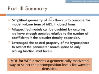
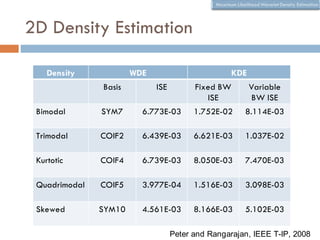
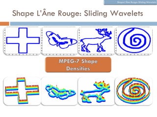
The document discusses using wavelet representations for density estimation and shape analysis. It proposes using a constrained maximum likelihood objective to estimate density coefficients in a multi-resolution wavelet basis. Model selection criteria like MDL, AIC and BIC are compared for selecting the number of resolution levels in the wavelet expansion, with MDL shown to be invariant to the multi-resolution analysis used. The criteria are tested on 1D densities with different shapes, with MDL and MSE performing best in distinguishing the densities.

1. SQUARE-ROOT WAVELET
DENSITIES AND SHAPE ANALYSIS
Anand Rangarajan, Center for Vision, Graphics and Medical Imaging
(CVGMI), University of Florida, Gainesville

2. Square-root densities
Walking the straight and narrow….on a sphere

3. Square-root densities
Wavelets
∞
p( x) = ∑
k
α j0 , k φ j0 , k ( x) + ∑ β j ,kψ
j ≥ j0 , k
j ,k ( x)
Shape is a point on hypersphere
due to Fisher-Rao geometry

4. Wavelet Representations
Father Mother
 Wavelets can approximate any f∊ℒ2, i.e.
∞
f ( x) = ∑ α j0 , k φ j0 , k ( x) + ∑ β j ,kψ
j ≥ j0 , k
j ,k ( x)
Translation index k Resolution level
 Only work with compactly supported, orthogonal
basis families: Haar, Daubechies, Symlets, Coiflets

5. Expand p, Not p !
 Expand in multi-resolution basis:
∞
p( x) = ∑ k
α j0 , k φ j0 , k ( x) + ∑ β j ,kψ
j ≥ j0 , k
j ,k ( x)
 Integrability constraints: ∞
h(α j0 , k , β j ,k ) = ∑ k
α 2
j0 , k + ∑ β
j ≥ j0 , k
2
j ,k =1
 Estimate coefficients using a constrained maximum
likelihood objective:
(  
)
N ∞
L (Θ ) = − log ∏ p ( xi | Θ ) + λ  ∑ α j ,k + ∑ β j ,k − 1
2 2 2
  0
i= 1  k j ≥ j0 , k 
Asymptotic Hessian of
negative log likelihood E{ H Objective is
L
convex
}= 4I where Θ = α { j0 , k ,β j ,k }

6. 2D Density Estimation
Density WDE KDE
Basis ISE Fixed BW Variable
ISE BW ISE
Bimodal SYM7 6.773E-03 1.752E-02 8.114E-03
Trimodal COIF2 6.439E-03 6.621E-03 1.037E-02
Kurtotic COIF4 6.739E-03 8.050E-03 7.470E-03
Quadrimodal COIF5 3.977E-04 1.516E-03 3.098E-03
Skewed SYM10 4.561E-03 8.166E-03 5.102E-03
Peter and Rangarajan, IEEE T-IP, 2008

7. Shape L’Âne Rouge: Sliding Wavelets

9. How Do We Select the Number of
Levels?
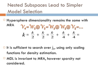
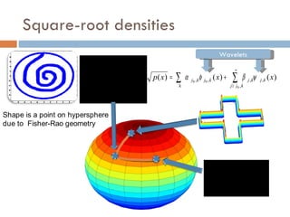
 In the wavelet expansion of p we need set j0
(starting level) and j1 (ending level)
j 1
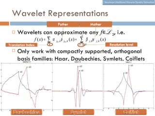
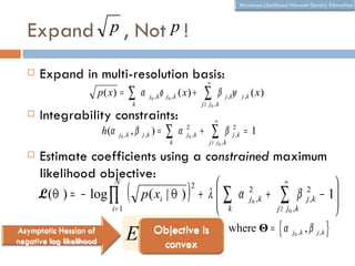
p( x) = ∑ k
α j0 , k φ j0 , k ( x) + ∑ β j ,kψ
j > j0 , k
j ,k ( x)
 Balasubramanian [32] proposed geometric
approach by analyzing the posterior of a model
class p(M) ∫ p(Θ ) p( E | Θ )dΘ
p(M | E ) =
p( E )
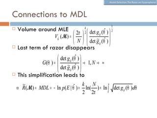
 The model selection criterion (razor) is
 ~
 det g ij (Θˆ ) 
ˆ (Mk =ln( ln p( E | Θˆ ) +det g V Θ M )Θ  +
N ( 1 
Total volume of manifold
R(M ) = − ln p( E | Θ ) + ) − ) + ln ∫ ln ij ( )d
R ln 
2 2π  V ˆ (M )  2 Volume ofg ij (Θˆ ) 
 det distinguishable
 Θ  
distributions around ML
Scales with Volume of model Ratio of expected Fisher
ML fit parameters and class manifold to empirical Fisher
samples.

10. Connections to MDL
1
 Volume around MLE k
 2π   det g ij (Θˆ ) 
2
2
VΘˆ (M ) =   ~
 N   det g ij (Θˆ ) 
 Last term of razor disappears
 det gij (Θˆ ) 
G(Θ ) =  ~
 → 1, N → ∞
 det gij (Θˆ ) 
 
 This simplification leads to
~ ˆ ) + k ln( N ) + ln det g (Θ )dΘ
⇒ R (M ) = MDL = − ln p( E | Θ
2 2π ∫ ij

11. Geometric Intuition
e rs
re f
z or p .
Th e ra these
Space of distributions Counting volumes

12. MDL for Wavelet Densities on the
Hypersphere
saupto50Color
Space of distributions

13. Intuition Behind Shrinking Surface Area
 Volume gets pushed into corners as dimensions
increase.
d Vs/Vc
1 1
2 .785
3 .524
4 .308
5 .164
6 .08
 In 100 dimensions diagonal of unit length for
sphere is only 10% of way to the cube diagonal.

14. Nested Subspaces Lead to Simpler
Model Selection
 Hypersphere dimensionality remains the same with
MRA
k k k k k
k= + = + + =
2 2 2 4 4
 It is sufficient to search over j0, using only scaling
functions for density estimation.
 MDL is invariant to MRA, however sparsity not
considered.

15. Other Model Selection Criteria
 Two-term MDL (MDL2) (Rissanen 1978)
MDL = − ln p( E | Θ
2 ˆ ) + k ln N 
2  2π 
 Akaike Information Criterion (AIC) (Akaike 1973)
AIC = − 2 ln p( E | Θˆ ) + 2k
 Bayesian Information Criterion (BIC) (Schwarz 1978)
BIC = − 2 ln p( E | Θˆ ) + 2k ln( N )
 Also compared to other distance measures
 Hellinger divergence (HELL)
 Mean Squared Error (MSE)
 L1

16. 1D Model Selection with Coiflets
Density
COIF1 (j0) COIF2 (j0)
MDL3 MDL2 AIC BIC MSE HELL L1 MDL3 MDL2 AIC BIC MSE HELL L1
Gaussian
0 0 1 0 1 1 1 -1 -1 0 -1 0 0 0
Skewed
Uni. 1 1 1 1 2 1 1 0 0 1 0 1 0 1
Str.
Skewed
Uni. 2 2 3 2 4 3 3 2 2 2 2 4 2 3
Kurtotic
Uni. 2 2 2 1 4 2 2 2 2 2 2 2 2 2
Outlier
2 2 3 2 5 3 4 2 2 2 2 4 2 4
Bimodal
1 0 1 0 2 1 1 0 0 0 0 1 0 1
Sep.
Bimodal 1 1 2 1 2 1 2 1 1 1 1 1 1 1
Skewed
Bimodal 1 1 1 1 2 2 2 1 1 1 1 1 1 1
Trimodal
1 1 1 1 1 1 1 1 1 1 1 1 2 1
Claw
2 2 2 2 2 2 2 2 2 2 2 2 2 2
Dbl. Claw
1 0 1 0 2 1 1 0 0 0 0 1 0 1
Asym.
Claw 2 1 2 1 3 2 3 2 1 2 1 3 2 3
Asym.
Dbl. Claw 1 1 1 0 2 1 2 0 0 2 0 2 2 2

17. MSE, j0=4 BIC, j0=0
MDL3 vs. BIC and MSE
MDL3, j0=2 MDL3, j0=1

18. Part III Summary
 Simplified geometry of p allows us to compute the
model volume term of MDL in closed form.
 Misspecified models can be avoided by assuring
we have enough samples relative to the number of
coefficients in the wavelet density expansion.
 Leveraged the nested property of the hypersphere
to restrict the parameter search space to only
scaling function start levels.
MDL for WDE provides a geometrically motivated
way to select the decomposition levels for wavelet
densities.

19. Shape L’Âne Rouge
A red donkey solves Klotski

20. Shape L’Âne Rouge: Sliding Wavelets

21. Geometry of Shape Matching
ap
oint Shape
on h is
ype
rsph
ere
Point set representation Wavelet density estimation
Fast Shape Similarity Using Hellinger Divergence
∫( ) 2
D( p1 || p2 ) = p(x | Θ 1 ) − p ( x | Θ 2 ) dx
(
= 2− 2 Θ 1Θ
T
2 )
Or Geodesic Distance
D( p1 , p2 ) = cos − 1 (Θ 1 Θ 2 )
T

22. Slidin
Localized Alignment Via
g
T T
 1 1 1   1 1 1 
 0 0 3 0 0 0 3 0 0 0 3 0 0 0 0 0  0 0 0 0 0 3 0 0 0 3 0 0 0 3 0 0
   
 Local shape differences will cause coefficients to
Permutations ⇒ Translations
shift.

 Slide coefficients back into alignment.

23. Penalize Excessive Sliding
 Location operator, r ( j , k ) , gives centroid of each (j,k) basis.
 Sliding cost equal to square of Euclidean distance.

24. Sliding Objective
 Objective minimizes over penalized permutation
assignments
  r
E (π ) = −  ∑ α j , kα j ,π ( k ) + ∑ β j , k β j ,π ( k ) 
(1)
0
( 2)
0
(1) ( 2)
 o n o pe
rato
tion  j0 , k j > j0 , k cati
ta  Lo 2
r mu + λ  ∑ r ( j0 , k ) − r ( π ( j0 , k ) ) + ∑ r ( j , k ) − r (π ( j , k ) ) 
2
P e
h t  j0 , k j ,k 
W e ig
 Solve
a lty via linear assignment using cost matrix
Pen
C = Θ 1Θ + λ D
T
Θiis vectorized list of ith shape’s coefficients and
2
 where
D is the matrix of distances between basis locations.

25. Effects of λ Peter and Rangarajan, CVPR 2008

26. Recognition Results on MPEG-7 DB
 All recognition rates are based on MPEG-7 bulls-
eye criterion.
 D2 shape distributions (Osada et al.) only at

27. Summary
 The geometry associated with the p wavelet
representation allows us to represent densities as
points on a unit hypersphere.
 For the first time, non-rigid alignment can be
addressed using linear assignment framework.
 Advantages of our method: no topological
restrictions, very little pre-processing, closed-form
metric.
Sliding wavelets provide a fast and accurate
method of shape matching