Download as PDF, PPTX


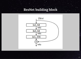
![U-Net Building Blocks (2)U-Net Building Blocks (2)
class up_block(nn.HybridBlock):
def __init__(self, channels, shrink=True, **kwargs):
super(up_block, self).__init__(**kwargs)
self.upsampler = nn.Conv2DTranspose(channels=channels, ker
strides=2, padding=1,
self.conv1 = conv_block(channels, 1)
self.conv3_0 = conv_block(channels, 3)
if shrink:
self.conv3_1 = conv_block(int(channels/2), 3)
else:
self.conv3_1 = conv_block(channels, 3)
def hybrid_forward(self, F, x, s):
x = self.upsampler(x)
x = self.conv1(x)
x = F.relu(x)
x = F.Crop(*[x,s], center crop=True)
23](https://image.slidesharecdn.com/largescalelanduseclassificationofsatelliteimagery-180620032048/85/Landuse-Classification-from-Satellite-Imagery-using-Deep-Learning-23-320.jpg)

![Cloud Classifier DoFnCloud Classifier DoFn
class FilterCloudyFn(apache_beam.DoFn):
def process(self, element):
"""
Returns clear images after filtering the cloudy ones
:param element:
:return:
"""
clear_images = []
batch = self.load_batch(element)
batch = batch.as_in_context(self.ctx)
preds = mx.nd.argmax(self.net(batch), axis=1)
idxs = np.arange(len(element))[preds.asnumpy() == 0]
clear_images.extend([element[i] for i in idxs])
yield clear_images
33](https://image.slidesharecdn.com/largescalelanduseclassificationofsatelliteimagery-180620032048/85/Landuse-Classification-from-Satellite-Imagery-using-Deep-Learning-33-320.jpg)
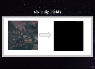
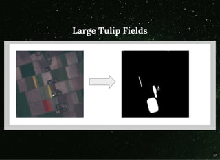
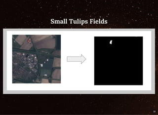


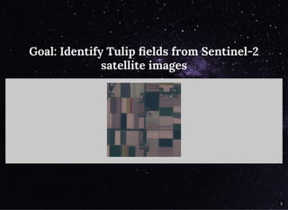
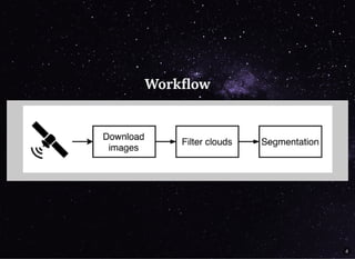
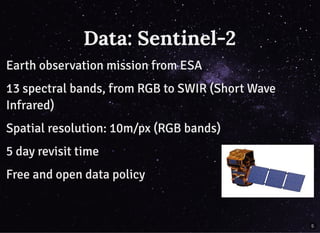
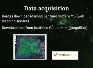
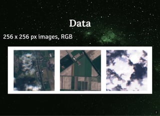
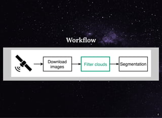
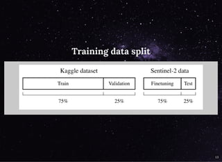
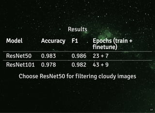
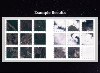
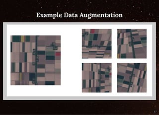
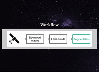
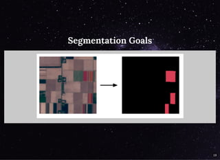
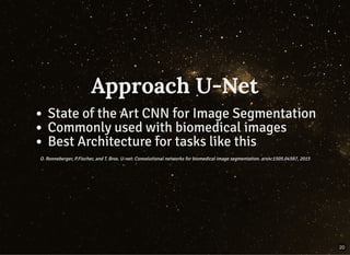
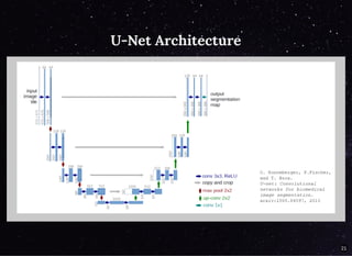
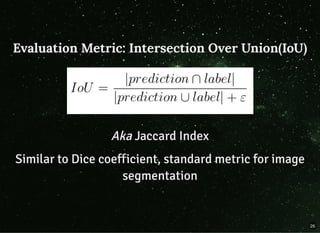
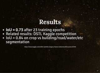
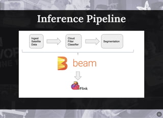
The document discusses a workflow for large-scale land use classification using Sentinel-2 satellite imagery, focusing on the identification of tulip fields. It details the data acquisition process, the use of cloud filtering through neural networks (ResNet50), and the application of U-Net architecture for image segmentation. The results indicate high model accuracy for filtering and segmentation tasks, with future work planned for further applications in agricultural analysis.