![For quick literature review
Several review/survey papers and book chapters
[Salvi et al., 2002]
[Zhang, 2005]
[Remondino and Fraser, 2006]
Y. Oyamada (Keio Univ. and TUM) Camera Calibration April 3, 2012 3 / 44](https://image.slidesharecdn.com/cameracalibration-121219105826-phpapp02/85/Camera-calibration-3-320.jpg)
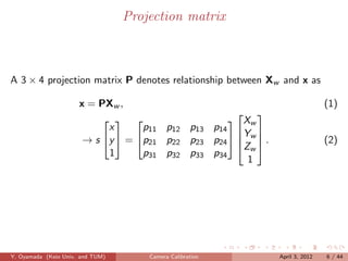
![Intrinsic and extrinsic parameters
A projection matrix can be decomposed into two components, intrinsic
and extrinsic parameters, as
x = PXw = A [R|t] Xw , (3)
Xw
x αx s x0 r11 r12 r13 t1
Y
→ y = 0 αy y0 r21 r22 r23 t2 w ,
Zw (4)
1 0 0 1 r31 r32 r33 t3
1
where
Intrinsic: 3 × 3 calibration matrix A.
Extrinsic: 3 × 3 Rotation matrix R and 3 × 1 translation vector t.
Y. Oyamada (Keio Univ. and TUM) Camera Calibration April 3, 2012 7 / 44](https://image.slidesharecdn.com/cameracalibration-121219105826-phpapp02/85/Camera-calibration-7-320.jpg)
![Extrinsic parameters
Denotes transformation between Xw and Xc as
Xc = [R|t] Xw , (5)
Xc X
r11 r12 r13 t1 w
Yc
= r21 r22 r23 t2 Yw . (6)
Zc Zw
r31 r32 r33 t3
1 1
Y. Oyamada (Keio Univ. and TUM) Camera Calibration April 3, 2012 8 / 44](https://image.slidesharecdn.com/cameracalibration-121219105826-phpapp02/85/Camera-calibration-8-320.jpg)
![Intrinsic parameters
Project a 3D point Xc to image plane as
x = A [R|t] Xw = AXc , (7)
Xc
x αx s x0
Y
→ y = 0 αy y0 c ,
Zc (8)
1 0 0 1
1
where
αx and αy are focal lengths in pixel unit.
x0 and y0 are image center in pixel unit.
s is skew parameter.
Y. Oyamada (Keio Univ. and TUM) Camera Calibration April 3, 2012 9 / 44](https://image.slidesharecdn.com/cameracalibration-121219105826-phpapp02/85/Camera-calibration-9-320.jpg)
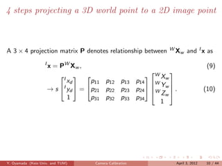
![1/4: A 3D world point to a 3D camera point
Change the world coordinate system to the camera one.
From a 3D point WX in metric system w.r.t. the world coordinate
w
To a 3D point C Xw in metric system w.r.t. the camera coordinate
C
Xw = [C Rw |C Tw ]W Xw , (11)
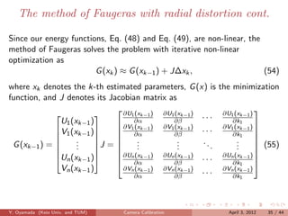
C
W Xw
Xw
C Y R11 R12 R13 t14 W
Y
→ s C w = R21 R22 R23 t24 W w .
Zw Zw (12)
R31 R32 R33 t34
1 1
Y. Oyamada (Keio Univ. and TUM) Camera Calibration April 3, 2012 11 / 44](https://image.slidesharecdn.com/cameracalibration-121219105826-phpapp02/85/Camera-calibration-11-320.jpg)
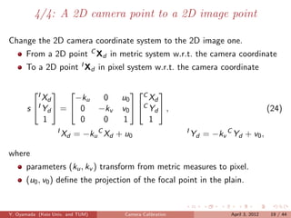
![2/4: A 3D camera point to a 2D camera point
Change the 3D camera coordinate system to the 2D camera one.
From a 3D point C Xw in metric system w.r.t. the camera coordinate
To a 2D point C Xu in metric system w.r.t. the camera coordinate
C
Xu = [C Rw |C Tw ]W Xw , (13)
W Xw
C
Xu f 0 0 0 W
Y
→ s C Yu = 0 f 0 0 W w ,
Zw (14)
1 0 0 1 0
1
C f W C f W
Xu = W Xw Yu = WZ
Yw ,
Zw w
where f denotes focal length in metric system.
Y. Oyamada (Keio Univ. and TUM) Camera Calibration April 3, 2012 12 / 44](https://image.slidesharecdn.com/cameracalibration-121219105826-phpapp02/85/Camera-calibration-12-320.jpg)
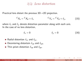
![3/4: Lens distortion: Radial distortion
Caused by flawed radial curvature of lens.
Modeled by [Tsai, 1987] 1 .
δxr = k1 C Xd (C Xd + C Yd )
2 2
δyr = k1 C Yd (C Xd + C Yd )
2 2
(17)
1
R. Y. Tsai. A versatile camera calibration technique for high-accuracy 3d machine vision metrology using off-the-shelf tv
cameras and lenses. IEEE Transactions on Robotics and Automation, 3(4):323–344, 1987
Y. Oyamada (Keio Univ. and TUM) Camera Calibration April 3, 2012 14 / 44](https://image.slidesharecdn.com/cameracalibration-121219105826-phpapp02/85/Camera-calibration-14-320.jpg)
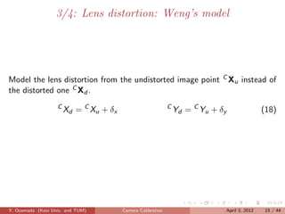
![3/4: Lens distortion: Decentering distortion
Since the optical center of the lens is not correctly aligned with the
center of the camera.
Modeled by [Weng et al., 1992] 2 ,
δxd = p1 (3C Xu + C Yu ) + 2p2 C Xu C Yu
2 2
(19)
δyd = 2p1 C Xu C Yu + p2 (C Xu + 3C Yu )
2 2
(20)
2
J. Weng, P. Cohen, and M. Herniou. Camera calibration with distortion models and accuracy evaluation. IEEE
Transactions on Pattern Analysis and Machine Intelligence, 14(10):965–980, 1992. ISSN 0162-8828. doi: 10.1109/34.159901.
URL http://dx.doi.org/10.1109/34.159901
Y. Oyamada (Keio Univ. and TUM) Camera Calibration April 3, 2012 16 / 44](https://image.slidesharecdn.com/cameracalibration-121219105826-phpapp02/85/Camera-calibration-16-320.jpg)
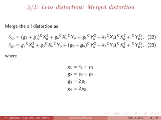
![3/4: Lens distortion: Thin prism distortion
From imperfection in lens design and manufacturing as well as camera
assembly.
Modeled by adding a thin prism to the optic system, causing radial
and tangential distortions [Weng et al., 1992].
δxp = s1 (C Xu + C Yu )
2 2
δyp = s2 (C Xu + C Yu )
2 2
(21)
Y. Oyamada (Keio Univ. and TUM) Camera Calibration April 3, 2012 17 / 44](https://image.slidesharecdn.com/cameracalibration-121219105826-phpapp02/85/Camera-calibration-17-320.jpg)
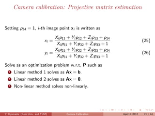
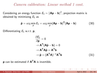
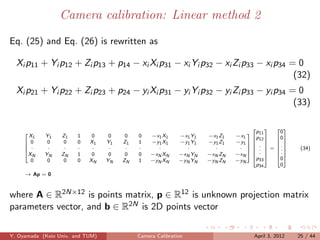
![Camera calibration: Linear method 1
Proposed by [Hall et al., 1982] 3 .
Eq. (25) and Eq. (26) is rewritten as
Xi p11 + Yi p12 + Zi p13 + p14 − xi Xi p31 − xi Yi p32 − xi Zi p33 = xi (27)
Xi p21 + Yi p22 + Zi p23 + p24 − yi Xi p31 − yi Yi p32 − yi Zi p33 = yi (28)
Given N corresponding points {Xi } and {xi }, generate following equation:
p11 x1
X1 Y1 Z1 1 0 0 0 0 −x1 X1 −x1 Y1 −x1 Z1 p
y1
0 0 0 0 X1 Y1 Z1 1 −y1 X1 −y1 Y1 12
−y1 Z1
. .
· · · · · · · · · · · . = . (29)
−xN ZN .
.
X
N YN ZN 1 0 0 0 0 −xN XN −xN YN p
x
0 0 0 0 XN YN ZN 1 −yN XN −yN YN −yN ZN 32 N
p33 yN
→ Ap = b
where A ∈ R2N×11 , p ∈ R11 , and b ∈ R2N .
3
E. L. Hall, J. B. K. Tio, C. A. McPherson, and F. A. Sadjadi. Measuring curved surfaces for robot vision. Computer, 15
(12):42–54, 1982. ISSN 0018-9162. doi: 10.1109/MC.1982.1653915. URL http://dx.doi.org/10.1109/MC.1982.1653915
Y. Oyamada (Keio Univ. and TUM) Camera Calibration April 3, 2012 22 / 44](https://image.slidesharecdn.com/cameracalibration-121219105826-phpapp02/85/Camera-calibration-22-320.jpg)
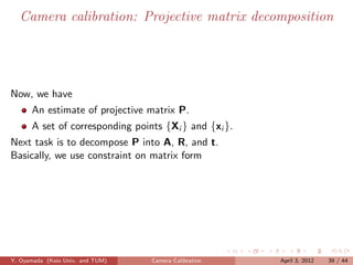
![Projective matrix decomposition cont.
Consider
P = A[R|t]
αx s x0 r11 r12 r13 t1
= 0 αy y0 r21 r22 r23 t2
0 0 1 r31 r32 r33 t3
T
αx s x0 r1 t1
= 0 αy y0 rT 2 t2
0 0 1 rT
3 t3
T T + x rT
αx r1 + sr2 0 3 αx tx + s · t2 + x0 tz
= αy rT + y0 rT
2 3 αx ty + y0 tz (58)
rT
3 tz
where rT = (rj1 , rj2 , rj3 ), for j = 1, 2, 3.
j
Y. Oyamada (Keio Univ. and TUM) Camera Calibration April 3, 2012 40 / 44](https://image.slidesharecdn.com/cameracalibration-121219105826-phpapp02/85/Camera-calibration-40-320.jpg)
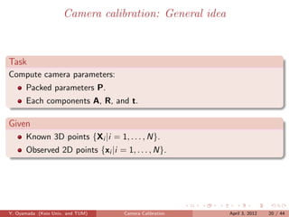
![Camera calibration methods
1 [Hall et al., 1982]
2 [Faugeras and Toscani, 1986]
3 [Salvi et al., 2002]
4 [Tsai, 1987]
5 [Weng et al., 1992]
Y. Oyamada (Keio Univ. and TUM) Camera Calibration April 3, 2012 42 / 44](https://image.slidesharecdn.com/cameracalibration-121219105826-phpapp02/85/Camera-calibration-42-320.jpg)

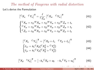
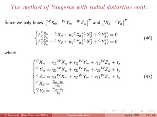
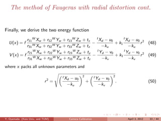
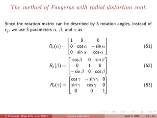
The document summarizes camera calibration techniques. It discusses: 1) Projecting 3D world points to 2D image points using a projection matrix with intrinsic and extrinsic parameters. 2) Computing camera parameters by estimating the projection matrix from known 3D points and corresponding 2D image points using linear and non-linear optimization methods. 3) Modeling lens distortion and different distortion types that must be accounted for during calibration.


![5G Explained! A High Level Overview [Introduction]](https://cdn.slidesharecdn.com/ss_thumbnails/5gexplainedahighleveloverview-260119165306-cc137a3e-thumbnail.jpg?width=640&height=640&fit=bounds)


