Matrices

A matrix is a rectangular array of real numbers.
Matrix A has 2 horizontal rows and 3 vertical columns.
3 1 −2 
A=
 7 −1 0.5

Each entry can be identified by its position in the
matrix.
7 is in Row 2 Column 1.
-2 is in Row 1 Column 3.
A matrix with m rows and n columns is of order m × n.
A is of order 2 × 3.
If m = n the matrix is said to be a square matrix of order n.
Copyright © by Houghton Mifflin Company, Inc. All rights reserved. 2

Examples: Find the order of each matrix

2 3 1 0  A has three rows and
A = 4
 2 1 4  four columns.

1
 1 6 2  The order of A is 3 × 4.


B has one row and five columns.
B = [ 2 5 2 −1 0] The order of B is 1 × 5.
B is called a row matrix.

3 1 
C=  C is a 2 × 2 square matrix.
6 2


An m × n matrix can be written
 a11 a12 L a1n 
a a22 L a2 n 
A = ai j  =  21
   M
.
M M 
 
am1 am1 am1 amn 

Two matrices A = [aij] and B = [bij] are equal if they
have the same order and aij = bij for every i and j.
0.5 9  1 
For example,  = 2 3  since both matrices
1 7  0.25 7 
 4
  
 
are of order 2 × 2 and all corresponding entries are equal.

Matrices
• Write a null matrix or Zero Matrix?
• Write a column matrix?


Matrices
• Diagonal Matrix – A square matrix whose
every element other than the diagonal
elements are ZERO is called a diagonal
matrix.
• Diagonal elements – The elements aij are
called diagonal elements when i=j


Matrices
• Scalar matrix -A diagonal matrix whose
diagonal elements are equal

• Identity Matrix (Unit matrix) – A diagonal
matrix whose diagonal elements are equal
to one


Matrices
• Triangular matrix – A square matrix whose
elements below or above the diagonal are
zero.
• What is an upper triangular matrix?
• What is a lower triangular matrix?


To add matrices:
1. Check to see if the matrices have the same order.
2. Add corresponding entries.
Example: Find the sums A + B and B + C.
1 5 
A= 2 1  B =  2 0 6  C = 3 −3 0 
  −1 0 −3 3 2 4 
0 6     
 
A has order 3 × 2 and B has order 2 × 3. So they cannot
be added. C has order 2 × 3 and can be added to B.
 2 0 6  3 −3 0  5 −3 6 
B+C =   + 3 2 4  =  2 2 1 
 −1 0 −3    

To subtract matrices:
1. Check to see if the matrices have the same order.
2. Subtract corresponding entries.
Example: Find the differences A – B and B – C.
3 7   2 −1  −1 5 1 
A=  B =  4 −5 C =  2 1 6 
2 1     
A and B are both of order 2 × 2 and can be subtracted.
 3 7   2 −1  1 8 
A−B =   −  4 −5 =  −2 6 
2 1     
Since B is of order 2 × 2 and C is of order 3 × 2,
they cannot be subtracted.

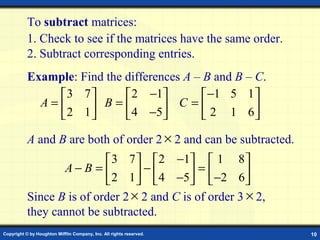
If A = [aij] is an m × n matrix and c is a scalar
(a real number), then the m × n matrix cA = [caij] is the
scalar multiple of A by c.  2 5 −1
3 4 0 
Example: Find 2A and –3A for A =  .
2 7
 2

 2(2) 2(5) 2( −1)   4 10 −2 
2 A =  2(3) 2(4) 2(0)  = 6 8 0 
   
 2(2) 2(7) 2(2)   4 14 4 
   
 −3(2) −3(5) −3( −1)   −6 −15 3 
1
− A =  −3(3) −3(4) −3(0)  =  −9 −12 0 
   
3
 −3(2) −3(7) −3(2)   −6 −21 −6 
   

Example: Calculate the value of 3A – 2B + C with
 2 −1 5 2 5 2
A = 3 5  B = 1 0  and C = 1 0 
     
 4 −2 
   3 −1 
   3 −1 
 

 2 −1 5 2  5 2
3 A − 2 B + C = 3  3 5  − 2 1 0  +  1 0 
     
 4 −2 
   3 − 1   3 −1 
   
 6 −3  10 4  5 2  1 − 5
= 9 15 −  2
   0  + 1 0  =  8 15 
    
12 −6   6 −2   3 −1   9 − 5 
       


Multiplication of Matrices
• The product AB of two matrices A and B is
defined only when the number of columns
A is same as the number of rows of B.
• A = m x n matrix
• B = n x p matrix.
• The order of AB is m x p.


Multiplication of Matrices
• AB may not be equal to BA
• If product AB is defined product BA may
not be defined.
• If A is a square matrix then A can be
multiplied by itself.


Transpose of a Matrix
• Let A be a matrix. The matrix obtained by
interchanging the rows and columns is
called the transpose of the matrix A.


Symmetric and Skew Symmetric
Matrices
• For a square matrix A if A=AT then it is a
symmetric matrix.

For a square matrix A if A= -AT then it is a
skew symmetric matrix.

Square matrix A + AT symmetric
Square matrix A – AT is skew symmetric

• If square matrices AB= BA then A,B are
commutative
• If square matrices AB=-BA the A,B are anti
commutative
• If A2 = A then A is idempotent


Determinant of a matrix
• The square matrix A has a uniquely
determined determinant associated with the
matrix.
• The determinant of a product of a matrix is
the product of their determinants.


Singular and Non singular
matrices
• A square matrix A is singular if determinant
A is zero.
• A square matrix A is non singular is
determinant A is not equal to Zero.


Elementary Operations in matrices.

1. Interchange two rows or columns of a matrix.
2. Multiply a row or column of a matrix by a non
zero constant.
3. Add a multiple of one row or column of a matrix
to another.


What is the use of Elementary
operations
• A sequence of elementary row operations
transforms the matrix of a system into the
matrix of another system with the same
solutions as the original system.
• Take matrix A X B = AB
• If we make elementary row operation in AB
then it is equivalent to making the same
operation in A and multiplying it with B.

An augmented matrix and a coefficient matrix are
associated with each system of linear equations.

2 x + 3 y − z = 12
For the system 
 x − 8y = 16

2 3 - 1 12
The augmented matrix is  .
1 - 8 0 16

 2 3 −1
The coefficient matrix is  .
1 −8 0 


Example: Apply the elementary row operation R1 ↔ R2
to the augmented matrix of the system  x + 2 y = 8 .

3x − y = 10

Row Operation Augmented Matrix System
1 2 8  x + 2y = 8
3 
 -1 10 
 3x − y = 10
R1 ↔ R2 ↓ ↓
3 -1 10 3x − y = 10
1  
 2 8  x + 2y = 8

Note that the two systems are equivalent.

Example: Apply the elementary row operation 3R2

3x − y = 10

1 2 8  x + 2y = 8
3 
 -1 10 
 3x − y = 10
3R2 ↓ ↓
1 2 8 
9 -3 30
 


Example: Apply the row operation –3R1 + R2

3x − y = 10

1 2 8  x + 2y = 8
3 
 -1 10 
 3x − y = 10
–3R1 + R2 ↓ ↓
1 2 8  x + 2y = 8
0  
 -7 - 14 −7 y = −14


Matrices

More Related Content

What's hot

Similar to Matrices

Matrices