SlideShare a Scribd company logo
Mohamad Tafrikan (moh.tafrikan@gmail.com) Page 1
GAUSS AND JACOBY ELIMINATION METHOD
1) Solve the linear equation system follow using Gauss Method
{
Solution:
{
( , ( + ( ,
The linear equation system (1) is , where:
Since . We will use the Gauss formula:
and . The linear equation system (1) will be ,
we will compute values of .
( *
( *
( *
( *
( *
( *
Now presented by:
Mohamad Tafrikan (moh.tafrikan@gmail.com) Page 2
{
The linear equation system (2) is , where:
Since . We will use the Gauss formula:
and . The linear equation system (2) will be , we
will compute values of .
( *
( *
Now presented by:
{
We get , and then , we get: and .
using this formula to get :
{
( ∑ )
( ∑ ) ( )
( ∑ ) ( ( )*
So, solution for (1) is { }
Mohamad Tafrikan (moh.tafrikan@gmail.com) Page 3
2) Solve the linear equation system follow using Gauss Elimination Method
{
Solution:
{
By change of row:
[ ] ⃗⃗⃗⃗⃗⃗⃗⃗⃗⃗⃗⃗⃗⃗⃗⃗⃗⃗⃗⃗⃗⃗⃗⃗⃗⃗⃗⃗⃗⃗⃗⃗⃗⃗⃗⃗⃗⃗⃗⃗⃗⃗⃗⃗⃗⃗⃗⃗⃗⃗⃗⃗⃗⃗⃗⃗⃗⃗⃗⃗⃗⃗⃗⃗⃗⃗⃗⃗⃗⃗⃗⃗⃗⃗⃗ [ ]
[ ] [ ]
The linear equation system (1) will be , we will compute values of
by , where .
( *
( *
( *
( *
( *
( *
* + ⃗⃗⃗⃗⃗⃗⃗⃗⃗⃗⃗⃗⃗⃗⃗⃗⃗⃗⃗⃗⃗⃗⃗⃗⃗⃗⃗⃗⃗⃗⃗⃗⃗⃗⃗⃗⃗⃗⃗⃗⃗⃗⃗⃗⃗⃗⃗⃗⃗⃗⃗⃗⃗⃗⃗⃗⃗⃗⃗⃗⃗⃗⃗⃗⃗⃗⃗⃗⃗⃗⃗⃗⃗⃗⃗ * +
We get a new linear equation system , that is
* +
Mohamad Tafrikan (moh.tafrikan@gmail.com) Page 4
We will use the Gauss formula: and .
The linear equation system (2) will be , we will compute values of .
( *
( *
[ ]
Now presented by:
{
We get , , .
By change of column:
[ ] [ ]
The linear equation system (3) will be , we will compute values of
by , where .
( *
( *
( *
( *
( *
( *
* + ⃗⃗⃗⃗⃗⃗⃗⃗⃗⃗⃗⃗⃗⃗⃗⃗⃗⃗⃗⃗⃗⃗⃗⃗⃗⃗⃗⃗⃗⃗⃗⃗⃗⃗⃗⃗⃗⃗⃗⃗⃗⃗⃗⃗⃗⃗⃗⃗⃗⃗⃗⃗⃗⃗⃗⃗⃗⃗⃗⃗⃗⃗⃗⃗⃗⃗⃗⃗⃗⃗⃗⃗⃗⃗⃗⃗⃗⃗⃗⃗⃗⃗⃗⃗⃗⃗⃗⃗⃗⃗ [ ]
Mohamad Tafrikan (moh.tafrikan@gmail.com) Page 5
We get a new linear equation system , that is
[ ]
We will use the Gauss formula: and .
The linear equation system (2) will be , we will compute values of .
( *
( *
[ ]
Now presented by:
{
We get , , .
BY DECOMPOSITION
[ ] [ ] [ ]
Where each entry of is determined by:
{
∑
∑
We get each entry of and ,
{
∑
(
∑
+
Mohamad Tafrikan (moh.tafrikan@gmail.com) Page 6
If we have a system we can solve its system by Decomposition Assume
, defined:
[ ] [ ] [ ]
We get:
{
∑
And form of defined by
[ ] [ ] [ ]
So, we get the solutions of is
{
( ∑ )
Example 1: Solve this system
{
Solution:
(3)3 (2) 2 (5) 5 (6) 6
(-1) (4) (3) (5)
(1) (-1) (3) (1)
And then we get:
[ ], * + * +
And we get
[ ] [ ] [ ]
So we get solution
Exercise 2. No 3.
Mohamad Tafrikan (moh.tafrikan@gmail.com) Page 7
Solve this a linear equation system by Decomposition!
* + * + * +
Solution:
(1)1 (2) 2 (3) 3 (4) 4 (2)2
(1) (4) (9) (16) (10)
(1) (8) (27) (64) (44)
(1) (16) (81) (256) (190)
And we get
* + * + * +
So we get solution
Solution by MATLAB:
>> A=[1 2 3 4;1 4 9 16;1 8 27 64;1 16 81 256]
A =
1 2 3 4
1 4 9 16
1 8 27 64
1 16 81 256
>> b=[2;10;44;190]
b =
2
10
44
190
>> x=(Ab)'
x = -1.0000 1.0000 -1.0000 1.0000
JACOBI METHOD
Suppose a system n-equation,
{ (1)
Mohamad Tafrikan (moh.tafrikan@gmail.com) Page 8
If , Eq. (1) can we write:
{ (2)
Where , and
( *
[ ] [ ] (3)
So, solution of Eq. (1) is
(4)
Alghoritm for Jacobi Method:
1. ( ) with initial value ( )
2.
3.
( ∑ )
4. ‖ ‖
5. For
Example 1:
{
By using (4), we get:
{
With initial value , we get:
Mohamad Tafrikan (moh.tafrikan@gmail.com) Page 9
And the next we will calculate by using MS Excel, we obtain:
Table 1
0 0 0 0
1 7.2 8.3 8.4
2 9.71 10.7 11.5
3 10.57 11.571 12.482
4 10.8535 11.8534 12.8282
5 10.95098 11.95099 12.94138
6 10.983375 11.983374 12.980394
7 10.9944162 11.9944163 12.9933498
8 10.99811159 11.99811158 12.9977665
9 10.99936446 11.99936446 12.99924463
Assume , since ‖ ‖ ‖ ‖ , then,
process stopped. So, we get final solution:
, or .
GAUSS-SEIDEL METHOD
Suppose a system n-equation,
{ (5)
If , Eq. (1) can we write:
{
(6)
Where , and
Mohamad Tafrikan (moh.tafrikan@gmail.com) Page 10
[ ] [ ]
Solution of Eq.(5) is
(7)
Alghoritm for Gauss-Seidel Method:
1. ( ) with initial condition ( )
2.
3.

( ∑ )

( ∑ ∑ )

( ∑ )
4. ‖ ‖ , then
5. For
Example 2.
{
By using (6), with initial value , we get:
( )
( )
( )
And the next we will calculate by using MS Excel, we obtain:
Tabel 2
0 0 0 0
1 7.2 9.02 11.644
2 10.4308 11.67188 12.820536
Mohamad Tafrikan (moh.tafrikan@gmail.com) Page 11
3 10.9312952 11.95723672 12.97770638
4 10.99126495 11.99466777 12.99718654
5 10.99890409 11.99932772 12.99964636
6 10.99986204 11.99991548 12.9999555
Assume , since ‖ ‖ ‖ ‖
,then, process stopped. So, we get final solution:
, or
Exercise page 89 number (1)
Use Jacobi method and Gauss-Seidel method to solve this system:
[ ] [ ] [ ]
(8)
With initial condition:
 By using Jacobi method
By using (4), we get:
{
With initial condition , we get:
And the next we will calculate by using MS Excel, we obtain:
Tabel 1
0 0 0 0 0 0 0
Mohamad Tafrikan (moh.tafrikan@gmail.com) Page 12
1 1.2 -3 2 -1.42 0.8 0.8
2 1.206 -2.8636 3.2794 -1.646 0.44086 0.35914
3 1.147936 -2.5552898 3.1008986 -2.0192692 0.87358 0.43272
4 1.09169802 -2.62921629
3.54091715
2
-
1.977922984
0.86700482
2 0.006575178
5
1.00131316
5 -2.58155443
3.54377891
4
-
2.061826638
1.01538009
7 0.148375275
6
0.96179561
3 -2.601802339
3.70257364
1
-
2.036178359
1.04463921
6 0.029259119
7
0.91266332
7 -2.595286119
3.72566523
2
-
2.060214779
1.10538006
8 0.060740852
8
0.89030797
2 -2.602097962
3.79128381
5
-
2.049953094
1.12595881
4 0.020578746
9
0.86655543
6 -2.601469385
3.80838238
3
-
2.057964588
1.15297405
7 0.027015243
1
0
0.85467021
6 -2.604128265
3.83723832
1
-
2.054246735
1.16461871
4 0.011644657
1
1
0.84339169
7 -2.604307402
3.84744106
3
-
2.057105832
1.17706750
4 0.012448789
1
2
0.83724727
6 -2.605423563 3.86053428
-
2.055810531
1.18325222
1 0.006184718
Assume , since ‖ ‖ ‖ ‖ ,
then, process stopped. So, we get final solution:
,
or .
 By using Gauss-Seidel method
By using (6), with initial value , we get:
( )
( )
( )
( )
( )
And the next we will calculate by using MS Excel, we obtain:
Mohamad Tafrikan (moh.tafrikan@gmail.com) Page 13
Tabel 1
0 0 0 0 0 0 0
1 1.2 -2.8636 2 -1.42 0.8 0.8
2 1.19236 -2.55979 3.260304 -1.66919 0.46814 0.33186
3 1.117419 -2.6365 3.091333 -2.06055 0.930169 0.462029324
4 1.091481 -2.57466 3.618334 -1.94957 0.853079 0.077090124
5 0.977438 -2.60858 3.514119 -2.09152 1.053798 0.200718593
6 0.96397 -2.59109 3.752752 -2.01513 1.033902 0.019895339
7 0.899536 -2.60569 3.706912 -2.07598 1.124904 0.091001323
8 0.89202 -2.59942 3.816874 -2.03865 1.120177 0.004726487
Assume , since ‖ ‖ ‖ ‖ , then,
process stopped. So, we get final solution:
, or
.
LAGRANGE INTERPOLATION
Suppose the data pair in [ ]available, the Lagrange interpolation is
the n-order polynomial interpolation, such that
Mohamad Tafrikan (moh.tafrikan@gmail.com) Page 14
Thus, the Lagrange interpolation results at the observation point are equal to the observed
value of itself. At point x which is not the point of observation Lagrange value is calculated
through the following formula:
∑
where ∏ ( ) is called coefficient of Lagrange.
Note that
{
So, for we get:
With the error is determined by the formula:
∏
So, the form of Lagrange interpolation for order-2 formula is as follows:
with a error determined as follows:
| |
Example 1.1
Given and a table of data pair :
10 11 12 13 14
Mohamad Tafrikan (moh.tafrikan@gmail.com) Page 15
2.302 6 2.397 9 2.484 9 2.564 9 2.639 1
By using Lagrange interpolation, find value of !
Solution:

First, we must compute , with


Then,
So,
With error:
, we get:
| |
Then

First, we must compute , with



Then,
Mohamad Tafrikan (moh.tafrikan@gmail.com) Page 16
So,
With error:
, we get:
| |
Then
Lagrange Interpolation Algorithm:
Declaration
Int ;
Real
Deskription
1. Input order polynomial (n)
2. Input pair for
3. Input point try xk;
4. Initial value ;
5. Load for i=0 to i=n
a. P(i)=1;
b. for j=0 to j=n
Mohamad Tafrikan (moh.tafrikan@gmail.com) Page 17
i. if then
c.
6. print (‘for x= ’, xk, ‘then y= ‘,L);
7. Stop
Program’s MATLAB Lagrange method
clear; help lagrang;
n = input('Order polinomial n = ');
x = zeros(n+1, 1);
y = zeros(n+1, 1);
z = zeros(n+1, 1);
for i = 1: n+1
fprintf('data ke-%2dn', i-1);
x(i) = input('x : ');
y(i) = input('y : ');
end
disp(' x y');
for i = 1: n+1
fprintf('%8.4f %10.6fn', x(i),y(i));
end
again=1;
while (lagi==1)
xk = input('input point xk: ');
L = 0;
for i = 1:n+1
P(i)=1;
for j= 1:n+1
if (i~=j)
P(i) = P(i)*(xk-x(j))/(x(i)-x(j));
end
end
L = L + P(i)*y(i);
end
fprintf('Value y= %10.8f on x= %8.6f n', L,xk);
disp(‘Press 1 to reload, Press 0 to exit');
again=input(' ');
end
Example 1.2
Estimate the error of √ at the point x=116 in the interval [100,144] using Lagrange
orde-2, calculated at , and .
Solution:
Mohamad Tafrikan (moh.tafrikan@gmail.com) Page 18
√ then
√
,
√
and
√
[ ]
√
|√ | ( *
Example 1.3
Draw the Lagrange chart for the following table, then estimate the value of y at point
x 1 3 5 7 9 11
y -3 4 5 -8 -3 0
>> myLAGRANG
input vektor sb-x: [1 3 5 7 9 11]
input vektor sb-y: [-3 4 5 -8 -3 0]
input point xk: 4.5
Value yk= 7.14111328 at xk= 4.500000
Mohamad Tafrikan (moh.tafrikan@gmail.com) Page 19
Example 1.4 : Interpolate at point x = 1.5 in the following observation table:
x -2 -1 1 2
y -6 0 0 6
>> myLAGRANG
Input vector sb-x: [-2 -1 1 2]
Input vector sb-y: [-6 0 0 6]
Input point xk: 1.5
Value yk= 1.87500000 at xk= 1.500000
Mohamad Tafrikan (moh.tafrikan@gmail.com) Page 20
NEWTON INTERPOLATION
Suppose is the -th Lagrange polynomial whose value corresponds to the value of
at points then model of divided difference of can written:
For coefficents that corresponds.
The coefficient or constant can be calculated in the following way:
 for , then
 for then such that
[ ]
using notation of divided difference:
 Divided Difference (Zeroth): [ ]
 Divided Difference (First): [ ]
{ [ ] [ ]}
 Divided Difference (Second):
[ ]
{ [ ] [ ]}
Mohamad Tafrikan (moh.tafrikan@gmail.com) Page 21
Divided Difference is more easily understood through the following table:
[ ] [ ] [ ] [ ] [ ]
[ ]
[ ]
{ [ ] [ ]}
[ ]
{ [ ] [ ]}
[ ]
[ ] [ ]
[ ]
[ ] [ ]
[ ]
[ ]
{ [ ] [ ]}
[ ]
{ [ ] [ ]}
[ ]
[ ] [ ]
[ ]
[ ]
{ [ ] [ ]}
[ ]
{ [ ] [ ]}
[ ]
[ ]
{ [ ] [ ]}
[ ]
-
Example 2.1
Given the following table. Look for the polynomial approach y value on x=2.
X -1 0 3 6 7
Y 3 -6 39 822 1611
Solution:
Consider the following Dived Difference table:
[ ]
[ ] [ ] [ ] [ ]
-
From the table, we get:
[ ] [ ] [ ] [ ] and
[ ] ; such that:
( ) ( ) ( ) ( )
So, for x=2, we obtain
Mohamad Tafrikan (moh.tafrikan@gmail.com) Page 22
Program’s MATLAB
clear; help NForward;
N = input(‘pait data : ');
T = zeros(N, N+1);
disp('input data: ');
for i = 1: N
fprintf('data th-%2dn', i);
x(i) = input('x : ');
y(i) = input('y : ');
T(i,1) = x(i);
T(i,2) = y(i);
end
for kol = 3:N+1
br = (N+2-kol);
for brs = 1:br
T(brs,kol)=T(brs+1, kol-1)-T(brs, kol-1);
end
end
disp(' x y delta1 delta2 ..........');
for i = 1: N
for j=1:N+1
fprintf('%8.4f ',T(i,j));
end
fprintf('n');
end
%interpolasi
lagi=1;
while (lagi==1)
h=x(2)-x(1);
xk = input(‘input point interpolation: ');
t = (xk - x(1))/h;
yk = T(1,2) + t*T(1,3);
for kol = (N+1):-1:4
fak = kol-2;
t1 = 1;
for j = (kol-3) : -1 : 1
t1 = t1*(t-j);
fak = fak*j;
end
t1 = t*t1;
yk = yk + t1*T(1,kol)/fak;
end
fprintf('At x= %8.6f value of y = %12.8f n',xk,yk);
disp(‘Press 1 to reload, Press 0 to exit');
lagi=input(' ');
end

More Related Content

What's hot

Gaussian Integration
Gaussian IntegrationGaussian Integration
Gaussian IntegrationReza Rahimi
 
Interpolation functions
Interpolation functionsInterpolation functions
Interpolation functionsTarun Gehlot
 
Computer fandamental bangla by soikot pdf
Computer fandamental bangla by soikot pdfComputer fandamental bangla by soikot pdf
Computer fandamental bangla by soikot pdfShifat Ahmed
 
HSC ICT c program question answer/program solve
HSC ICT c program question answer/program solveHSC ICT c program question answer/program solve
HSC ICT c program question answer/program solveAmirul Islam
 
Newton's Backward Interpolation Formula with Example
Newton's Backward Interpolation Formula with ExampleNewton's Backward Interpolation Formula with Example
Newton's Backward Interpolation Formula with ExampleMuhammadUsmanIkram2
 
Newton’s Forward & backward interpolation
Newton’s Forward &  backward interpolation Newton’s Forward &  backward interpolation
Newton’s Forward & backward interpolation Meet Patel
 
Gauss Elimination Method With Partial Pivoting
Gauss Elimination Method With Partial PivotingGauss Elimination Method With Partial Pivoting
Gauss Elimination Method With Partial PivotingSM. Aurnob
 
TOC 8 | Derivation, Parse Tree & Ambiguity Check
TOC 8 | Derivation, Parse Tree & Ambiguity CheckTOC 8 | Derivation, Parse Tree & Ambiguity Check
TOC 8 | Derivation, Parse Tree & Ambiguity CheckMohammad Imam Hossain
 
Thomas algorithm
Thomas algorithmThomas algorithm
Thomas algorithmParidhi SK
 
unit-4-dynamic programming
unit-4-dynamic programmingunit-4-dynamic programming
unit-4-dynamic programminghodcsencet
 
GATE Engineering Maths : System of Linear Equations
GATE Engineering Maths : System of Linear EquationsGATE Engineering Maths : System of Linear Equations
GATE Engineering Maths : System of Linear EquationsParthDave57
 
Newton backward interpolation
Newton backward interpolationNewton backward interpolation
Newton backward interpolationMUHAMMADUMAIR647
 
Numerical method for solving non linear equations
Numerical method for solving non linear equationsNumerical method for solving non linear equations
Numerical method for solving non linear equationsMdHaque78
 
Applied numerical methods lec10
Applied numerical methods lec10Applied numerical methods lec10
Applied numerical methods lec10Yasser Ahmed
 
Newton Cotes Integration Method, Open Newton Cotes, Closed Newton Cotes Gauss...
Newton Cotes Integration Method, Open Newton Cotes, Closed Newton Cotes Gauss...Newton Cotes Integration Method, Open Newton Cotes, Closed Newton Cotes Gauss...
Newton Cotes Integration Method, Open Newton Cotes, Closed Newton Cotes Gauss...HadiaZahid2
 

What's hot (20)

Gaussian Integration
Gaussian IntegrationGaussian Integration
Gaussian Integration
 
Interpolation functions
Interpolation functionsInterpolation functions
Interpolation functions
 
Computer fandamental bangla by soikot pdf
Computer fandamental bangla by soikot pdfComputer fandamental bangla by soikot pdf
Computer fandamental bangla by soikot pdf
 
HSC ICT c program question answer/program solve
HSC ICT c program question answer/program solveHSC ICT c program question answer/program solve
HSC ICT c program question answer/program solve
 
Computer fundamental full
Computer fundamental fullComputer fundamental full
Computer fundamental full
 
Newton's Backward Interpolation Formula with Example
Newton's Backward Interpolation Formula with ExampleNewton's Backward Interpolation Formula with Example
Newton's Backward Interpolation Formula with Example
 
TOC 10 | Turing Machine
TOC 10 | Turing MachineTOC 10 | Turing Machine
TOC 10 | Turing Machine
 
Newton’s Forward & backward interpolation
Newton’s Forward &  backward interpolation Newton’s Forward &  backward interpolation
Newton’s Forward & backward interpolation
 
Gauss Elimination Method With Partial Pivoting
Gauss Elimination Method With Partial PivotingGauss Elimination Method With Partial Pivoting
Gauss Elimination Method With Partial Pivoting
 
TOC 8 | Derivation, Parse Tree & Ambiguity Check
TOC 8 | Derivation, Parse Tree & Ambiguity CheckTOC 8 | Derivation, Parse Tree & Ambiguity Check
TOC 8 | Derivation, Parse Tree & Ambiguity Check
 
Thomas algorithm
Thomas algorithmThomas algorithm
Thomas algorithm
 
unit-4-dynamic programming
unit-4-dynamic programmingunit-4-dynamic programming
unit-4-dynamic programming
 
GATE Engineering Maths : System of Linear Equations
GATE Engineering Maths : System of Linear EquationsGATE Engineering Maths : System of Linear Equations
GATE Engineering Maths : System of Linear Equations
 
Newton backward interpolation
Newton backward interpolationNewton backward interpolation
Newton backward interpolation
 
Numerical method for solving non linear equations
Numerical method for solving non linear equationsNumerical method for solving non linear equations
Numerical method for solving non linear equations
 
Programming Language (chapter 5 for class 11 and 12)
Programming Language (chapter 5 for class 11 and 12)Programming Language (chapter 5 for class 11 and 12)
Programming Language (chapter 5 for class 11 and 12)
 
MS Excel bengali complete tutorial with image
MS Excel bengali complete tutorial with imageMS Excel bengali complete tutorial with image
MS Excel bengali complete tutorial with image
 
Applied numerical methods lec10
Applied numerical methods lec10Applied numerical methods lec10
Applied numerical methods lec10
 
Sor
SorSor
Sor
 
Newton Cotes Integration Method, Open Newton Cotes, Closed Newton Cotes Gauss...
Newton Cotes Integration Method, Open Newton Cotes, Closed Newton Cotes Gauss...Newton Cotes Integration Method, Open Newton Cotes, Closed Newton Cotes Gauss...
Newton Cotes Integration Method, Open Newton Cotes, Closed Newton Cotes Gauss...
 

Similar to Jacobi method and lagrange interpolation

Engineering Mathematics-IV_B.Tech_Semester-IV_Unit-V
Engineering Mathematics-IV_B.Tech_Semester-IV_Unit-VEngineering Mathematics-IV_B.Tech_Semester-IV_Unit-V
Engineering Mathematics-IV_B.Tech_Semester-IV_Unit-VRai University
 
engineeringmathematics-iv_unit-v
engineeringmathematics-iv_unit-vengineeringmathematics-iv_unit-v
engineeringmathematics-iv_unit-vKundan Kumar
 
INVERSION OF MATRIX BY GAUSS ELIMINATION METHOD
INVERSION OF MATRIX BY GAUSS ELIMINATION METHODINVERSION OF MATRIX BY GAUSS ELIMINATION METHOD
INVERSION OF MATRIX BY GAUSS ELIMINATION METHODreach2arkaELECTRICAL
 
Week 9-Quadratic Function.pptx
Week 9-Quadratic Function.pptxWeek 9-Quadratic Function.pptx
Week 9-Quadratic Function.pptxLyaniCebrian1
 
Numerical solution of linear volterra fredholm integro-
Numerical solution of linear volterra fredholm integro-Numerical solution of linear volterra fredholm integro-
Numerical solution of linear volterra fredholm integro-Alexander Decker
 
Sixth order hybrid block method for the numerical solution of first order ini...
Sixth order hybrid block method for the numerical solution of first order ini...Sixth order hybrid block method for the numerical solution of first order ini...
Sixth order hybrid block method for the numerical solution of first order ini...Alexander Decker
 
Uniform Order Legendre Approach for Continuous Hybrid Block Methods for the S...
Uniform Order Legendre Approach for Continuous Hybrid Block Methods for the S...Uniform Order Legendre Approach for Continuous Hybrid Block Methods for the S...
Uniform Order Legendre Approach for Continuous Hybrid Block Methods for the S...IOSR Journals
 
Derivation and Application of Six-Point Linear Multistep Numerical Method for...
Derivation and Application of Six-Point Linear Multistep Numerical Method for...Derivation and Application of Six-Point Linear Multistep Numerical Method for...
Derivation and Application of Six-Point Linear Multistep Numerical Method for...IOSR Journals
 
Solving Quadratic Equation by Completing the Square.pptx
Solving Quadratic Equation by Completing the Square.pptxSolving Quadratic Equation by Completing the Square.pptx
Solving Quadratic Equation by Completing the Square.pptxDebbieranteErmac
 
Numerical solution of system of linear equations
Numerical solution of system of linear equationsNumerical solution of system of linear equations
Numerical solution of system of linear equationsreach2arkaELECTRICAL
 
Simultaneous Equations Practical Construction
Simultaneous Equations Practical ConstructionSimultaneous Equations Practical Construction
Simultaneous Equations Practical ConstructionDaniel Ross
 
Solution of matlab chapter 3
Solution of matlab chapter 3Solution of matlab chapter 3
Solution of matlab chapter 3AhsanIrshad8
 
dddddddddddddddddddddddddddddddddddddddddddddddddddddAlgorithm.pptx
dddddddddddddddddddddddddddddddddddddddddddddddddddddAlgorithm.pptxdddddddddddddddddddddddddddddddddddddddddddddddddddddAlgorithm.pptx
dddddddddddddddddddddddddddddddddddddddddddddddddddddAlgorithm.pptxSubramaniyanChandras1
 
WCS Specialist Maths An Introduction to Matrices PowerPoint
WCS Specialist Maths An Introduction to Matrices PowerPointWCS Specialist Maths An Introduction to Matrices PowerPoint
WCS Specialist Maths An Introduction to Matrices PowerPointKingp18
 
Solving First Derivative Equation
Solving First Derivative EquationSolving First Derivative Equation
Solving First Derivative EquationAulia Khalqillah
 
Ch 1 Final 10Math.pdf
Ch 1 Final 10Math.pdfCh 1 Final 10Math.pdf
Ch 1 Final 10Math.pdfHabibDawar3
 

Similar to Jacobi method and lagrange interpolation (20)

Engineering Mathematics-IV_B.Tech_Semester-IV_Unit-V
Engineering Mathematics-IV_B.Tech_Semester-IV_Unit-VEngineering Mathematics-IV_B.Tech_Semester-IV_Unit-V
Engineering Mathematics-IV_B.Tech_Semester-IV_Unit-V
 
engineeringmathematics-iv_unit-v
engineeringmathematics-iv_unit-vengineeringmathematics-iv_unit-v
engineeringmathematics-iv_unit-v
 
INVERSION OF MATRIX BY GAUSS ELIMINATION METHOD
INVERSION OF MATRIX BY GAUSS ELIMINATION METHODINVERSION OF MATRIX BY GAUSS ELIMINATION METHOD
INVERSION OF MATRIX BY GAUSS ELIMINATION METHOD
 
Ca 1.6
Ca 1.6Ca 1.6
Ca 1.6
 
Week 9-Quadratic Function.pptx
Week 9-Quadratic Function.pptxWeek 9-Quadratic Function.pptx
Week 9-Quadratic Function.pptx
 
Numerical solution of linear volterra fredholm integro-
Numerical solution of linear volterra fredholm integro-Numerical solution of linear volterra fredholm integro-
Numerical solution of linear volterra fredholm integro-
 
Sixth order hybrid block method for the numerical solution of first order ini...
Sixth order hybrid block method for the numerical solution of first order ini...Sixth order hybrid block method for the numerical solution of first order ini...
Sixth order hybrid block method for the numerical solution of first order ini...
 
Uniform Order Legendre Approach for Continuous Hybrid Block Methods for the S...
Uniform Order Legendre Approach for Continuous Hybrid Block Methods for the S...Uniform Order Legendre Approach for Continuous Hybrid Block Methods for the S...
Uniform Order Legendre Approach for Continuous Hybrid Block Methods for the S...
 
Derivation and Application of Six-Point Linear Multistep Numerical Method for...
Derivation and Application of Six-Point Linear Multistep Numerical Method for...Derivation and Application of Six-Point Linear Multistep Numerical Method for...
Derivation and Application of Six-Point Linear Multistep Numerical Method for...
 
Mqm em
Mqm emMqm em
Mqm em
 
Chapter001
Chapter001Chapter001
Chapter001
 
Solving Quadratic Equation by Completing the Square.pptx
Solving Quadratic Equation by Completing the Square.pptxSolving Quadratic Equation by Completing the Square.pptx
Solving Quadratic Equation by Completing the Square.pptx
 
Numerical solution of system of linear equations
Numerical solution of system of linear equationsNumerical solution of system of linear equations
Numerical solution of system of linear equations
 
Simultaneous Equations Practical Construction
Simultaneous Equations Practical ConstructionSimultaneous Equations Practical Construction
Simultaneous Equations Practical Construction
 
Solution of matlab chapter 3
Solution of matlab chapter 3Solution of matlab chapter 3
Solution of matlab chapter 3
 
Calculus Homework Help
Calculus Homework HelpCalculus Homework Help
Calculus Homework Help
 
dddddddddddddddddddddddddddddddddddddddddddddddddddddAlgorithm.pptx
dddddddddddddddddddddddddddddddddddddddddddddddddddddAlgorithm.pptxdddddddddddddddddddddddddddddddddddddddddddddddddddddAlgorithm.pptx
dddddddddddddddddddddddddddddddddddddddddddddddddddddAlgorithm.pptx
 
WCS Specialist Maths An Introduction to Matrices PowerPoint
WCS Specialist Maths An Introduction to Matrices PowerPointWCS Specialist Maths An Introduction to Matrices PowerPoint
WCS Specialist Maths An Introduction to Matrices PowerPoint
 
Solving First Derivative Equation
Solving First Derivative EquationSolving First Derivative Equation
Solving First Derivative Equation
 
Ch 1 Final 10Math.pdf
Ch 1 Final 10Math.pdfCh 1 Final 10Math.pdf
Ch 1 Final 10Math.pdf
 

Recently uploaded

RNA INTERFERENCE: UNRAVELING GENETIC SILENCING
RNA INTERFERENCE: UNRAVELING GENETIC SILENCINGRNA INTERFERENCE: UNRAVELING GENETIC SILENCING
RNA INTERFERENCE: UNRAVELING GENETIC SILENCINGAADYARAJPANDEY1
 
Earliest Galaxies in the JADES Origins Field: Luminosity Function and Cosmic ...
Earliest Galaxies in the JADES Origins Field: Luminosity Function and Cosmic ...Earliest Galaxies in the JADES Origins Field: Luminosity Function and Cosmic ...
Earliest Galaxies in the JADES Origins Field: Luminosity Function and Cosmic ...Sérgio Sacani
 
Pests of sugarcane_Binomics_IPM_Dr.UPR.pdf
Pests of sugarcane_Binomics_IPM_Dr.UPR.pdfPests of sugarcane_Binomics_IPM_Dr.UPR.pdf
Pests of sugarcane_Binomics_IPM_Dr.UPR.pdfPirithiRaju
 
Richard's entangled aventures in wonderland
Richard's entangled aventures in wonderlandRichard's entangled aventures in wonderland
Richard's entangled aventures in wonderlandRichard Gill
 
insect taxonomy importance systematics and classification
insect taxonomy importance systematics and classificationinsect taxonomy importance systematics and classification
insect taxonomy importance systematics and classificationanitaento25
 
INSIGHT Partner Profile: Tampere University
INSIGHT Partner Profile: Tampere UniversityINSIGHT Partner Profile: Tampere University
INSIGHT Partner Profile: Tampere UniversitySteffi Friedrichs
 
Topography and sediments of the floor of the Bay of Bengal
Topography and sediments of the floor of the Bay of BengalTopography and sediments of the floor of the Bay of Bengal
Topography and sediments of the floor of the Bay of BengalMd Hasan Tareq
 
Structures and textures of metamorphic rocks
Structures and textures of metamorphic rocksStructures and textures of metamorphic rocks
Structures and textures of metamorphic rockskumarmathi863
 
Circulatory system_ Laplace law. Ohms law.reynaults law,baro-chemo-receptors-...
Circulatory system_ Laplace law. Ohms law.reynaults law,baro-chemo-receptors-...Circulatory system_ Laplace law. Ohms law.reynaults law,baro-chemo-receptors-...
Circulatory system_ Laplace law. Ohms law.reynaults law,baro-chemo-receptors-...muralinath2
 
EY - Supply Chain Services 2018_template.pptx
EY - Supply Chain Services 2018_template.pptxEY - Supply Chain Services 2018_template.pptx
EY - Supply Chain Services 2018_template.pptxAlguinaldoKong
 
In silico drugs analogue design: novobiocin analogues.pptx
In silico drugs analogue design: novobiocin analogues.pptxIn silico drugs analogue design: novobiocin analogues.pptx
In silico drugs analogue design: novobiocin analogues.pptxAlaminAfendy1
 
Anemia_ different types_causes_ conditions
Anemia_ different types_causes_ conditionsAnemia_ different types_causes_ conditions
Anemia_ different types_causes_ conditionsmuralinath2
 
Predicting property prices with machine learning algorithms.pdf
Predicting property prices with machine learning algorithms.pdfPredicting property prices with machine learning algorithms.pdf
Predicting property prices with machine learning algorithms.pdfbinhminhvu04
 
Transport in plants G1.pptx Cambridge IGCSE
Transport in plants G1.pptx Cambridge IGCSETransport in plants G1.pptx Cambridge IGCSE
Transport in plants G1.pptx Cambridge IGCSEjordanparish425
 
Comparative structure of adrenal gland in vertebrates
Comparative structure of adrenal gland in vertebratesComparative structure of adrenal gland in vertebrates
Comparative structure of adrenal gland in vertebratessachin783648
 
Mammalian Pineal Body Structure and Also Functions
Mammalian Pineal Body Structure and Also FunctionsMammalian Pineal Body Structure and Also Functions
Mammalian Pineal Body Structure and Also FunctionsYOGESH DOGRA
 
A Giant Impact Origin for the First Subduction on Earth
A Giant Impact Origin for the First Subduction on EarthA Giant Impact Origin for the First Subduction on Earth
A Giant Impact Origin for the First Subduction on EarthSérgio Sacani
 
Musical Meetups Knowledge Graph (MMKG): a collection of evidence for historic...
Musical Meetups Knowledge Graph (MMKG): a collection of evidence for historic...Musical Meetups Knowledge Graph (MMKG): a collection of evidence for historic...
Musical Meetups Knowledge Graph (MMKG): a collection of evidence for historic...Alba Morales
 
The ASGCT Annual Meeting was packed with exciting progress in the field advan...
The ASGCT Annual Meeting was packed with exciting progress in the field advan...The ASGCT Annual Meeting was packed with exciting progress in the field advan...
The ASGCT Annual Meeting was packed with exciting progress in the field advan...Health Advances
 
Astronomy Update- Curiosity’s exploration of Mars _ Local Briefs _ leadertele...
Astronomy Update- Curiosity’s exploration of Mars _ Local Briefs _ leadertele...Astronomy Update- Curiosity’s exploration of Mars _ Local Briefs _ leadertele...
Astronomy Update- Curiosity’s exploration of Mars _ Local Briefs _ leadertele...NathanBaughman3
 

Recently uploaded (20)

RNA INTERFERENCE: UNRAVELING GENETIC SILENCING
RNA INTERFERENCE: UNRAVELING GENETIC SILENCINGRNA INTERFERENCE: UNRAVELING GENETIC SILENCING
RNA INTERFERENCE: UNRAVELING GENETIC SILENCING
 
Earliest Galaxies in the JADES Origins Field: Luminosity Function and Cosmic ...
Earliest Galaxies in the JADES Origins Field: Luminosity Function and Cosmic ...Earliest Galaxies in the JADES Origins Field: Luminosity Function and Cosmic ...
Earliest Galaxies in the JADES Origins Field: Luminosity Function and Cosmic ...
 
Pests of sugarcane_Binomics_IPM_Dr.UPR.pdf
Pests of sugarcane_Binomics_IPM_Dr.UPR.pdfPests of sugarcane_Binomics_IPM_Dr.UPR.pdf
Pests of sugarcane_Binomics_IPM_Dr.UPR.pdf
 
Richard's entangled aventures in wonderland
Richard's entangled aventures in wonderlandRichard's entangled aventures in wonderland
Richard's entangled aventures in wonderland
 
insect taxonomy importance systematics and classification
insect taxonomy importance systematics and classificationinsect taxonomy importance systematics and classification
insect taxonomy importance systematics and classification
 
INSIGHT Partner Profile: Tampere University
INSIGHT Partner Profile: Tampere UniversityINSIGHT Partner Profile: Tampere University
INSIGHT Partner Profile: Tampere University
 
Topography and sediments of the floor of the Bay of Bengal
Topography and sediments of the floor of the Bay of BengalTopography and sediments of the floor of the Bay of Bengal
Topography and sediments of the floor of the Bay of Bengal
 
Structures and textures of metamorphic rocks
Structures and textures of metamorphic rocksStructures and textures of metamorphic rocks
Structures and textures of metamorphic rocks
 
Circulatory system_ Laplace law. Ohms law.reynaults law,baro-chemo-receptors-...
Circulatory system_ Laplace law. Ohms law.reynaults law,baro-chemo-receptors-...Circulatory system_ Laplace law. Ohms law.reynaults law,baro-chemo-receptors-...
Circulatory system_ Laplace law. Ohms law.reynaults law,baro-chemo-receptors-...
 
EY - Supply Chain Services 2018_template.pptx
EY - Supply Chain Services 2018_template.pptxEY - Supply Chain Services 2018_template.pptx
EY - Supply Chain Services 2018_template.pptx
 
In silico drugs analogue design: novobiocin analogues.pptx
In silico drugs analogue design: novobiocin analogues.pptxIn silico drugs analogue design: novobiocin analogues.pptx
In silico drugs analogue design: novobiocin analogues.pptx
 
Anemia_ different types_causes_ conditions
Anemia_ different types_causes_ conditionsAnemia_ different types_causes_ conditions
Anemia_ different types_causes_ conditions
 
Predicting property prices with machine learning algorithms.pdf
Predicting property prices with machine learning algorithms.pdfPredicting property prices with machine learning algorithms.pdf
Predicting property prices with machine learning algorithms.pdf
 
Transport in plants G1.pptx Cambridge IGCSE
Transport in plants G1.pptx Cambridge IGCSETransport in plants G1.pptx Cambridge IGCSE
Transport in plants G1.pptx Cambridge IGCSE
 
Comparative structure of adrenal gland in vertebrates
Comparative structure of adrenal gland in vertebratesComparative structure of adrenal gland in vertebrates
Comparative structure of adrenal gland in vertebrates
 
Mammalian Pineal Body Structure and Also Functions
Mammalian Pineal Body Structure and Also FunctionsMammalian Pineal Body Structure and Also Functions
Mammalian Pineal Body Structure and Also Functions
 
A Giant Impact Origin for the First Subduction on Earth
A Giant Impact Origin for the First Subduction on EarthA Giant Impact Origin for the First Subduction on Earth
A Giant Impact Origin for the First Subduction on Earth
 
Musical Meetups Knowledge Graph (MMKG): a collection of evidence for historic...
Musical Meetups Knowledge Graph (MMKG): a collection of evidence for historic...Musical Meetups Knowledge Graph (MMKG): a collection of evidence for historic...
Musical Meetups Knowledge Graph (MMKG): a collection of evidence for historic...
 
The ASGCT Annual Meeting was packed with exciting progress in the field advan...
The ASGCT Annual Meeting was packed with exciting progress in the field advan...The ASGCT Annual Meeting was packed with exciting progress in the field advan...
The ASGCT Annual Meeting was packed with exciting progress in the field advan...
 
Astronomy Update- Curiosity’s exploration of Mars _ Local Briefs _ leadertele...
Astronomy Update- Curiosity’s exploration of Mars _ Local Briefs _ leadertele...Astronomy Update- Curiosity’s exploration of Mars _ Local Briefs _ leadertele...
Astronomy Update- Curiosity’s exploration of Mars _ Local Briefs _ leadertele...
 

Jacobi method and lagrange interpolation

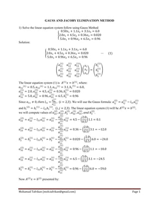
  • 1. Mohamad Tafrikan (moh.tafrikan@gmail.com) Page 1 GAUSS AND JACOBY ELIMINATION METHOD 1) Solve the linear equation system follow using Gauss Method { Solution: { ( , ( + ( , The linear equation system (1) is , where: Since . We will use the Gauss formula: and . The linear equation system (1) will be , we will compute values of . ( * ( * ( * ( * ( * ( * Now presented by:
  • 2. Mohamad Tafrikan (moh.tafrikan@gmail.com) Page 2 { The linear equation system (2) is , where: Since . We will use the Gauss formula: and . The linear equation system (2) will be , we will compute values of . ( * ( * Now presented by: { We get , and then , we get: and . using this formula to get : { ( ∑ ) ( ∑ ) ( ) ( ∑ ) ( ( )* So, solution for (1) is { }
  • 3. Mohamad Tafrikan (moh.tafrikan@gmail.com) Page 3 2) Solve the linear equation system follow using Gauss Elimination Method { Solution: { By change of row: [ ] ⃗⃗⃗⃗⃗⃗⃗⃗⃗⃗⃗⃗⃗⃗⃗⃗⃗⃗⃗⃗⃗⃗⃗⃗⃗⃗⃗⃗⃗⃗⃗⃗⃗⃗⃗⃗⃗⃗⃗⃗⃗⃗⃗⃗⃗⃗⃗⃗⃗⃗⃗⃗⃗⃗⃗⃗⃗⃗⃗⃗⃗⃗⃗⃗⃗⃗⃗⃗⃗⃗⃗⃗⃗⃗⃗ [ ] [ ] [ ] The linear equation system (1) will be , we will compute values of by , where . ( * ( * ( * ( * ( * ( * * + ⃗⃗⃗⃗⃗⃗⃗⃗⃗⃗⃗⃗⃗⃗⃗⃗⃗⃗⃗⃗⃗⃗⃗⃗⃗⃗⃗⃗⃗⃗⃗⃗⃗⃗⃗⃗⃗⃗⃗⃗⃗⃗⃗⃗⃗⃗⃗⃗⃗⃗⃗⃗⃗⃗⃗⃗⃗⃗⃗⃗⃗⃗⃗⃗⃗⃗⃗⃗⃗⃗⃗⃗⃗⃗⃗ * + We get a new linear equation system , that is * +
  • 4. Mohamad Tafrikan (moh.tafrikan@gmail.com) Page 4 We will use the Gauss formula: and . The linear equation system (2) will be , we will compute values of . ( * ( * [ ] Now presented by: { We get , , . By change of column: [ ] [ ] The linear equation system (3) will be , we will compute values of by , where . ( * ( * ( * ( * ( * ( * * + ⃗⃗⃗⃗⃗⃗⃗⃗⃗⃗⃗⃗⃗⃗⃗⃗⃗⃗⃗⃗⃗⃗⃗⃗⃗⃗⃗⃗⃗⃗⃗⃗⃗⃗⃗⃗⃗⃗⃗⃗⃗⃗⃗⃗⃗⃗⃗⃗⃗⃗⃗⃗⃗⃗⃗⃗⃗⃗⃗⃗⃗⃗⃗⃗⃗⃗⃗⃗⃗⃗⃗⃗⃗⃗⃗⃗⃗⃗⃗⃗⃗⃗⃗⃗⃗⃗⃗⃗⃗⃗ [ ]
  • 5. Mohamad Tafrikan (moh.tafrikan@gmail.com) Page 5 We get a new linear equation system , that is [ ] We will use the Gauss formula: and . The linear equation system (2) will be , we will compute values of . ( * ( * [ ] Now presented by: { We get , , . BY DECOMPOSITION [ ] [ ] [ ] Where each entry of is determined by: { ∑ ∑ We get each entry of and , { ∑ ( ∑ +
  • 6. Mohamad Tafrikan (moh.tafrikan@gmail.com) Page 6 If we have a system we can solve its system by Decomposition Assume , defined: [ ] [ ] [ ] We get: { ∑ And form of defined by [ ] [ ] [ ] So, we get the solutions of is { ( ∑ ) Example 1: Solve this system { Solution: (3)3 (2) 2 (5) 5 (6) 6 (-1) (4) (3) (5) (1) (-1) (3) (1) And then we get: [ ], * + * + And we get [ ] [ ] [ ] So we get solution Exercise 2. No 3.
  • 7. Mohamad Tafrikan (moh.tafrikan@gmail.com) Page 7 Solve this a linear equation system by Decomposition! * + * + * + Solution: (1)1 (2) 2 (3) 3 (4) 4 (2)2 (1) (4) (9) (16) (10) (1) (8) (27) (64) (44) (1) (16) (81) (256) (190) And we get * + * + * + So we get solution Solution by MATLAB: >> A=[1 2 3 4;1 4 9 16;1 8 27 64;1 16 81 256] A = 1 2 3 4 1 4 9 16 1 8 27 64 1 16 81 256 >> b=[2;10;44;190] b = 2 10 44 190 >> x=(Ab)' x = -1.0000 1.0000 -1.0000 1.0000 JACOBI METHOD Suppose a system n-equation, { (1)
  • 8. Mohamad Tafrikan (moh.tafrikan@gmail.com) Page 8 If , Eq. (1) can we write: { (2) Where , and ( * [ ] [ ] (3) So, solution of Eq. (1) is (4) Alghoritm for Jacobi Method: 1. ( ) with initial value ( ) 2. 3. ( ∑ ) 4. ‖ ‖ 5. For Example 1: { By using (4), we get: { With initial value , we get:
  • 9. Mohamad Tafrikan (moh.tafrikan@gmail.com) Page 9 And the next we will calculate by using MS Excel, we obtain: Table 1 0 0 0 0 1 7.2 8.3 8.4 2 9.71 10.7 11.5 3 10.57 11.571 12.482 4 10.8535 11.8534 12.8282 5 10.95098 11.95099 12.94138 6 10.983375 11.983374 12.980394 7 10.9944162 11.9944163 12.9933498 8 10.99811159 11.99811158 12.9977665 9 10.99936446 11.99936446 12.99924463 Assume , since ‖ ‖ ‖ ‖ , then, process stopped. So, we get final solution: , or . GAUSS-SEIDEL METHOD Suppose a system n-equation, { (5) If , Eq. (1) can we write: { (6) Where , and
  • 10. Mohamad Tafrikan (moh.tafrikan@gmail.com) Page 10 [ ] [ ] Solution of Eq.(5) is (7) Alghoritm for Gauss-Seidel Method: 1. ( ) with initial condition ( ) 2. 3.  ( ∑ )  ( ∑ ∑ )  ( ∑ ) 4. ‖ ‖ , then 5. For Example 2. { By using (6), with initial value , we get: ( ) ( ) ( ) And the next we will calculate by using MS Excel, we obtain: Tabel 2 0 0 0 0 1 7.2 9.02 11.644 2 10.4308 11.67188 12.820536
  • 11. Mohamad Tafrikan (moh.tafrikan@gmail.com) Page 11 3 10.9312952 11.95723672 12.97770638 4 10.99126495 11.99466777 12.99718654 5 10.99890409 11.99932772 12.99964636 6 10.99986204 11.99991548 12.9999555 Assume , since ‖ ‖ ‖ ‖ ,then, process stopped. So, we get final solution: , or Exercise page 89 number (1) Use Jacobi method and Gauss-Seidel method to solve this system: [ ] [ ] [ ] (8) With initial condition:  By using Jacobi method By using (4), we get: { With initial condition , we get: And the next we will calculate by using MS Excel, we obtain: Tabel 1 0 0 0 0 0 0 0
  • 12. Mohamad Tafrikan (moh.tafrikan@gmail.com) Page 12 1 1.2 -3 2 -1.42 0.8 0.8 2 1.206 -2.8636 3.2794 -1.646 0.44086 0.35914 3 1.147936 -2.5552898 3.1008986 -2.0192692 0.87358 0.43272 4 1.09169802 -2.62921629 3.54091715 2 - 1.977922984 0.86700482 2 0.006575178 5 1.00131316 5 -2.58155443 3.54377891 4 - 2.061826638 1.01538009 7 0.148375275 6 0.96179561 3 -2.601802339 3.70257364 1 - 2.036178359 1.04463921 6 0.029259119 7 0.91266332 7 -2.595286119 3.72566523 2 - 2.060214779 1.10538006 8 0.060740852 8 0.89030797 2 -2.602097962 3.79128381 5 - 2.049953094 1.12595881 4 0.020578746 9 0.86655543 6 -2.601469385 3.80838238 3 - 2.057964588 1.15297405 7 0.027015243 1 0 0.85467021 6 -2.604128265 3.83723832 1 - 2.054246735 1.16461871 4 0.011644657 1 1 0.84339169 7 -2.604307402 3.84744106 3 - 2.057105832 1.17706750 4 0.012448789 1 2 0.83724727 6 -2.605423563 3.86053428 - 2.055810531 1.18325222 1 0.006184718 Assume , since ‖ ‖ ‖ ‖ , then, process stopped. So, we get final solution: , or .  By using Gauss-Seidel method By using (6), with initial value , we get: ( ) ( ) ( ) ( ) ( ) And the next we will calculate by using MS Excel, we obtain:
  • 13. Mohamad Tafrikan (moh.tafrikan@gmail.com) Page 13 Tabel 1 0 0 0 0 0 0 0 1 1.2 -2.8636 2 -1.42 0.8 0.8 2 1.19236 -2.55979 3.260304 -1.66919 0.46814 0.33186 3 1.117419 -2.6365 3.091333 -2.06055 0.930169 0.462029324 4 1.091481 -2.57466 3.618334 -1.94957 0.853079 0.077090124 5 0.977438 -2.60858 3.514119 -2.09152 1.053798 0.200718593 6 0.96397 -2.59109 3.752752 -2.01513 1.033902 0.019895339 7 0.899536 -2.60569 3.706912 -2.07598 1.124904 0.091001323 8 0.89202 -2.59942 3.816874 -2.03865 1.120177 0.004726487 Assume , since ‖ ‖ ‖ ‖ , then, process stopped. So, we get final solution: , or . LAGRANGE INTERPOLATION Suppose the data pair in [ ]available, the Lagrange interpolation is the n-order polynomial interpolation, such that
  • 14. Mohamad Tafrikan (moh.tafrikan@gmail.com) Page 14 Thus, the Lagrange interpolation results at the observation point are equal to the observed value of itself. At point x which is not the point of observation Lagrange value is calculated through the following formula: ∑ where ∏ ( ) is called coefficient of Lagrange. Note that { So, for we get: With the error is determined by the formula: ∏ So, the form of Lagrange interpolation for order-2 formula is as follows: with a error determined as follows: | | Example 1.1 Given and a table of data pair : 10 11 12 13 14
  • 15. Mohamad Tafrikan (moh.tafrikan@gmail.com) Page 15 2.302 6 2.397 9 2.484 9 2.564 9 2.639 1 By using Lagrange interpolation, find value of ! Solution:  First, we must compute , with   Then, So, With error: , we get: | | Then  First, we must compute , with    Then,
  • 16. Mohamad Tafrikan (moh.tafrikan@gmail.com) Page 16 So, With error: , we get: | | Then Lagrange Interpolation Algorithm: Declaration Int ; Real Deskription 1. Input order polynomial (n) 2. Input pair for 3. Input point try xk; 4. Initial value ; 5. Load for i=0 to i=n a. P(i)=1; b. for j=0 to j=n
  • 17. Mohamad Tafrikan (moh.tafrikan@gmail.com) Page 17 i. if then c. 6. print (‘for x= ’, xk, ‘then y= ‘,L); 7. Stop Program’s MATLAB Lagrange method clear; help lagrang; n = input('Order polinomial n = '); x = zeros(n+1, 1); y = zeros(n+1, 1); z = zeros(n+1, 1); for i = 1: n+1 fprintf('data ke-%2dn', i-1); x(i) = input('x : '); y(i) = input('y : '); end disp(' x y'); for i = 1: n+1 fprintf('%8.4f %10.6fn', x(i),y(i)); end again=1; while (lagi==1) xk = input('input point xk: '); L = 0; for i = 1:n+1 P(i)=1; for j= 1:n+1 if (i~=j) P(i) = P(i)*(xk-x(j))/(x(i)-x(j)); end end L = L + P(i)*y(i); end fprintf('Value y= %10.8f on x= %8.6f n', L,xk); disp(‘Press 1 to reload, Press 0 to exit'); again=input(' '); end Example 1.2 Estimate the error of √ at the point x=116 in the interval [100,144] using Lagrange orde-2, calculated at , and . Solution:
  • 18. Mohamad Tafrikan (moh.tafrikan@gmail.com) Page 18 √ then √ , √ and √ [ ] √ |√ | ( * Example 1.3 Draw the Lagrange chart for the following table, then estimate the value of y at point x 1 3 5 7 9 11 y -3 4 5 -8 -3 0 >> myLAGRANG input vektor sb-x: [1 3 5 7 9 11] input vektor sb-y: [-3 4 5 -8 -3 0] input point xk: 4.5 Value yk= 7.14111328 at xk= 4.500000
  • 19. Mohamad Tafrikan (moh.tafrikan@gmail.com) Page 19 Example 1.4 : Interpolate at point x = 1.5 in the following observation table: x -2 -1 1 2 y -6 0 0 6 >> myLAGRANG Input vector sb-x: [-2 -1 1 2] Input vector sb-y: [-6 0 0 6] Input point xk: 1.5 Value yk= 1.87500000 at xk= 1.500000
  • 20. Mohamad Tafrikan (moh.tafrikan@gmail.com) Page 20 NEWTON INTERPOLATION Suppose is the -th Lagrange polynomial whose value corresponds to the value of at points then model of divided difference of can written: For coefficents that corresponds. The coefficient or constant can be calculated in the following way:  for , then  for then such that [ ] using notation of divided difference:  Divided Difference (Zeroth): [ ]  Divided Difference (First): [ ] { [ ] [ ]}  Divided Difference (Second): [ ] { [ ] [ ]}
  • 21. Mohamad Tafrikan (moh.tafrikan@gmail.com) Page 21 Divided Difference is more easily understood through the following table: [ ] [ ] [ ] [ ] [ ] [ ] [ ] { [ ] [ ]} [ ] { [ ] [ ]} [ ] [ ] [ ] [ ] [ ] [ ] [ ] [ ] { [ ] [ ]} [ ] { [ ] [ ]} [ ] [ ] [ ] [ ] [ ] { [ ] [ ]} [ ] { [ ] [ ]} [ ] [ ] { [ ] [ ]} [ ] - Example 2.1 Given the following table. Look for the polynomial approach y value on x=2. X -1 0 3 6 7 Y 3 -6 39 822 1611 Solution: Consider the following Dived Difference table: [ ] [ ] [ ] [ ] [ ] - From the table, we get: [ ] [ ] [ ] [ ] and [ ] ; such that: ( ) ( ) ( ) ( ) So, for x=2, we obtain
  • 22. Mohamad Tafrikan (moh.tafrikan@gmail.com) Page 22 Program’s MATLAB clear; help NForward; N = input(‘pait data : '); T = zeros(N, N+1); disp('input data: '); for i = 1: N fprintf('data th-%2dn', i); x(i) = input('x : '); y(i) = input('y : '); T(i,1) = x(i); T(i,2) = y(i); end for kol = 3:N+1 br = (N+2-kol); for brs = 1:br T(brs,kol)=T(brs+1, kol-1)-T(brs, kol-1); end end disp(' x y delta1 delta2 ..........'); for i = 1: N for j=1:N+1 fprintf('%8.4f ',T(i,j)); end fprintf('n'); end %interpolasi lagi=1; while (lagi==1) h=x(2)-x(1); xk = input(‘input point interpolation: '); t = (xk - x(1))/h; yk = T(1,2) + t*T(1,3); for kol = (N+1):-1:4 fak = kol-2; t1 = 1; for j = (kol-3) : -1 : 1 t1 = t1*(t-j); fak = fak*j; end t1 = t*t1; yk = yk + t1*T(1,kol)/fak; end fprintf('At x= %8.6f value of y = %12.8f n',xk,yk); disp(‘Press 1 to reload, Press 0 to exit'); lagi=input(' '); end