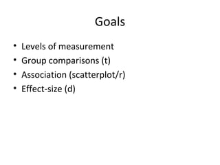
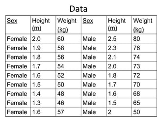
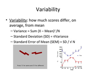
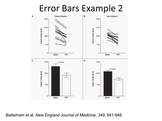
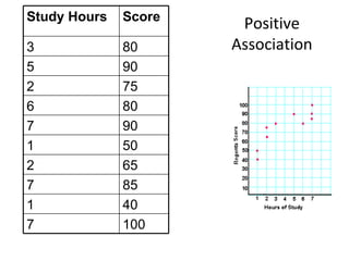
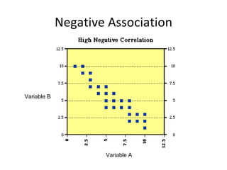
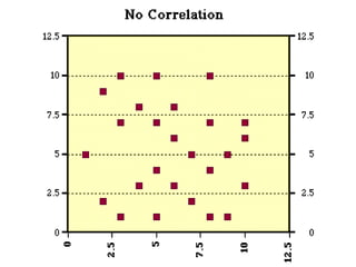
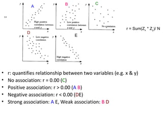
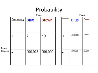
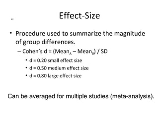
The document discusses various statistical concepts and analyses including levels of measurement, group comparisons using t-tests, assessing relationships between variables through scatterplots and the correlation coefficient r, and calculating effect sizes using Cohen's d to summarize results across multiple studies. Examples are provided of different types of data, computing means, variability, and interpreting statistical significance when comparing groups.

1. ψ
Statistics
Brian J. Piper, Ph.D.

2. Mark Twain (?)
• There are three types of lies, lies, damn lies,
and statistics.
http://en.wikipedia.org/wiki/Lies,_damned_lies,_and_statistics

3. Goals
• Levels of measurement
• Group comparisons (t)
• Association (scatterplot/r)
• Effect-size (d)

4. )
Levels of Measurement
• Nominal: categorical, example: sex
• Ratio: quantitative, example: age
• Ordinal: ranking, example: self-report
– Strongly disagree = 1
– Disagree = 2
– Neutral = 3
– Agree = 4
– Strongly agree = 5
– S.D.-------------------------------------------------------------------------------------------S.A.

5. What do these countries have in
common?
• Liberia
• Burma
• United States

6. Metric System
Unit Symbol Factor
tera T 1 x 1012
giga G 1 x 109
kilo K 1 x 103
--- -- 1
centi c 1 x 10-2
milli m 1 x 10-3
micro μ 1 x 10-6

7. Data
Sex Height Weight Sex Height Weight
(m) (kg) (m) (kg)
Female 2.0 60 Male 2.5 80
Female 1.9 58 Male 2.3 76
Female 1.8 56 Male 2.1 74
Female 1.7 54 Male 2.0 73
Female 1.6 52 Male 1.8 72
Female 1.5 50 Male 1.7 70
Female 1.4 48 Male 1.6 68
Female 1.3 46 Male 1.5 65
Female 1.6 57 Male 2 50

8. Sex Height Weight Sex Height Weight
(m) (kg) (m) (kg)
Female 2.0 60 Male 2.5 80
Female 1.9 58 Male 2.3 76
Female 1.8 56 Male 2.1 74
Female 1.7 54 Male 2.0 73
Female 1.6 52 Male 1.8 72
Female 1.5 50 Male 1.7 70
Female 1.4 48 Male 1.6 68
Female 1.3 46 Male 1.5 65
Female 1.6 57 Male 2 50
Average 1.64 53.4 1.94 69.8
Mean (or average) = Sum (X) /N where N is the # of scores

9. Variability
• Variability: how much scores differ, on
average, from mean
– Variance = Sum (X – Mean)2 /N
– Standard Deviation (SD) = √Variance
– Standard Error of Mean (SEM) = SD / √ N

10. Group Comparisons I
• Are women lighter then men?
– P = probability value
if p < .05 therefore statistically “significant”
– t test = (MeanMales - MeanFemales) / SEM
– t = 4.97, p = .0001
90
80 ►
←
70
WEIGHT
←
►
60
→
50 SEX_
female
40 male
9876543210123456789
Count Count

11. Group Comparisons II
• Do men have a higher IQ then women?
• T is the measure of variability (e.g. S.E.M.)
A. Sample Size = 40 B. Sample Size = 4,000 C. Sample Size = 4,000 ( * p < .05).
→
125 125 105
100 100
100
75 75 *
IQ
IQ
IQ
50 50
95
25 25
0 0 90
Men (N = 20) Women (N=20) Men (N = 2000) Women (N=2000) Men (N = 2000) Women (N=2000)
A finding with a * refers to a “statistically significant” finding, e.g. men > women

12. Error Bars Example 2
Batterham et al. New England Journal of Medicine, 349, 941-948.

13. Scatterplots
64 90
60 80
WEIGHT_MALE
Outlier? ->
WEIGHT_F
56 70
52 60
48 50 Outlier? ->
44 40
1.3 1.4 1.5 1.6 1.7 1.8 1.9 2.0 1.4 1.6 1.8 2.0 2.2 2.4 2.6
HEIGHT_F HEIGHT_M

14. Study Hours Score
Positive
3 80 Association
5 90
2 75
6 80
7 90
1 50
2 65
7 85
1 40
7 100

15. Negative Association
Variable B
Variable A

17. 3.1
Standardized “Z” Scores
• Z is a #
• Z = 0 therefore average
• Z > 0 therefore above average
• Z < 0 therefore below average
• Z = (X – Mean) / SD
• Z = (600 – 500) / 100
= 1.0

18. B C
A
3.6
r = Sum(Zx * Zy)/ N
D
E
• r: quantifies relationship between two variables (e.g. x & y)
• No association: r = 0.00 (C)
• Positive association: r > 0.00 (A B)
• Negative association: r < 0.00 (DE)
• Strong association: A E, Weak association: B D

19. Probability
Eyes Eyes
Probability
Frequency Blue Brown Blue Brown
.000002 .000010
+ 2 10 +
Brain
Cancer .999998 .99999
- 999,998 999,990 -

20. 3.2
Risk
• Absolute Risk: Rate of condition/total
population studied, e.g. .000002 or .000010
.0002% or .0010%
• Relative Risk: Rate of condition among group
A divided by rate of condition among group B
– .000010 = 5.0
________
.0000002

21. 4.3
Effect-Size
• Procedure used to summarize the magnitude
of group differences.
– Cohen’s d = (MeanA – MeanB) / SD
• d = 0.20 small effect size
• d = 0.50 medium effect size
• d = 0.80 large effect size
Can be averaged for multiple studies (meta-analysis).

22. Summary
Goal Intuition Test
Difference in Bar Graphs with “t-test”
means SEM
Relationship between
variables (ratio x ratio)
Scatterplot Correlation “r”
Summarize Read papers Effect size
many studies “Cohen’s d”