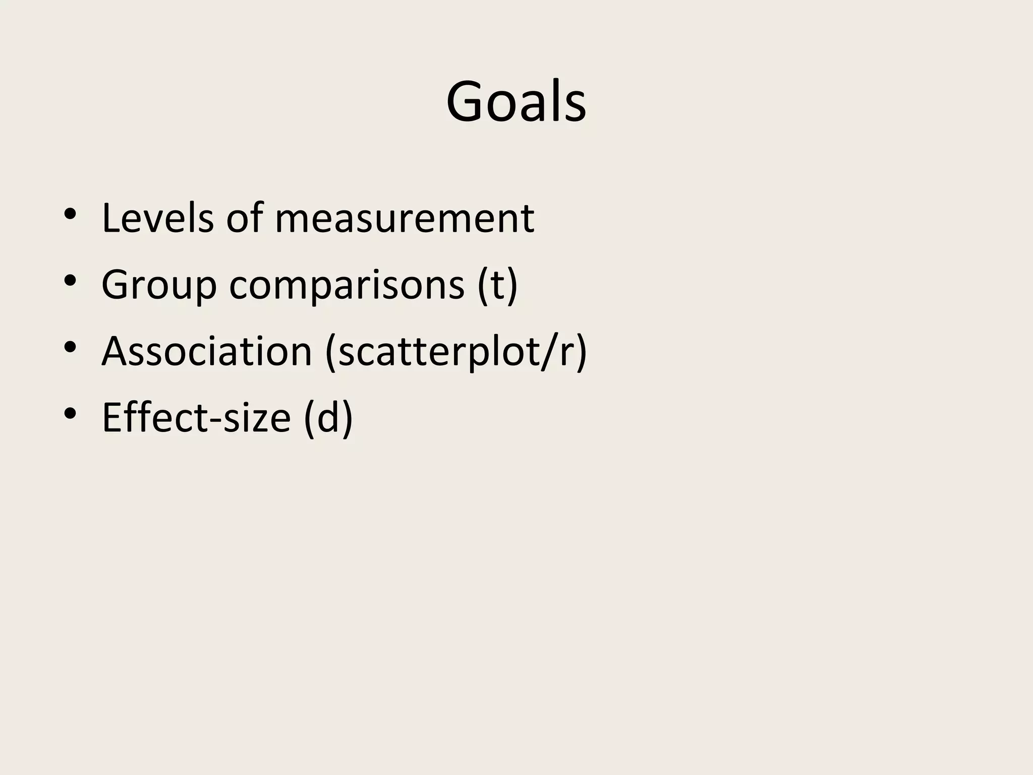
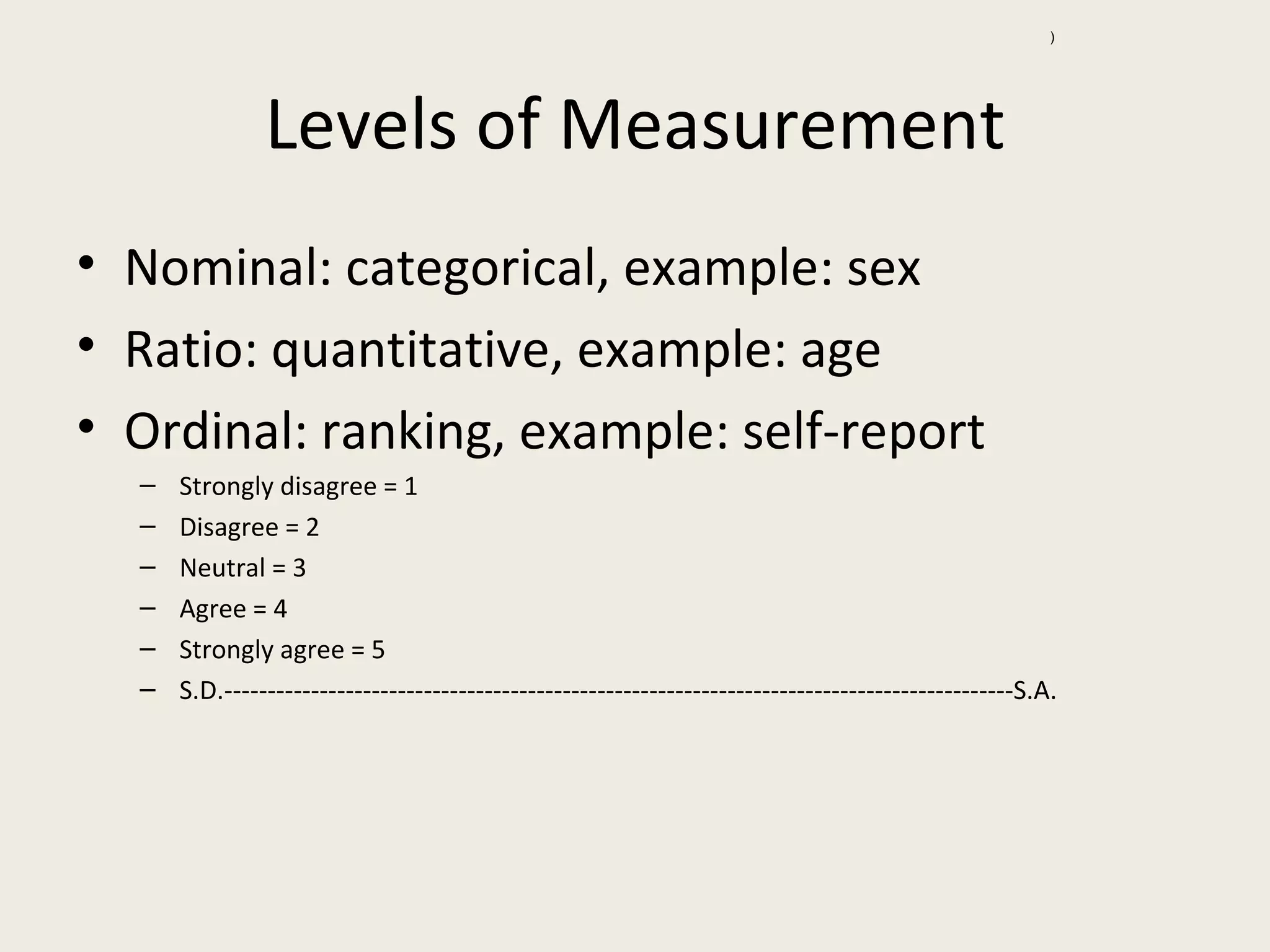
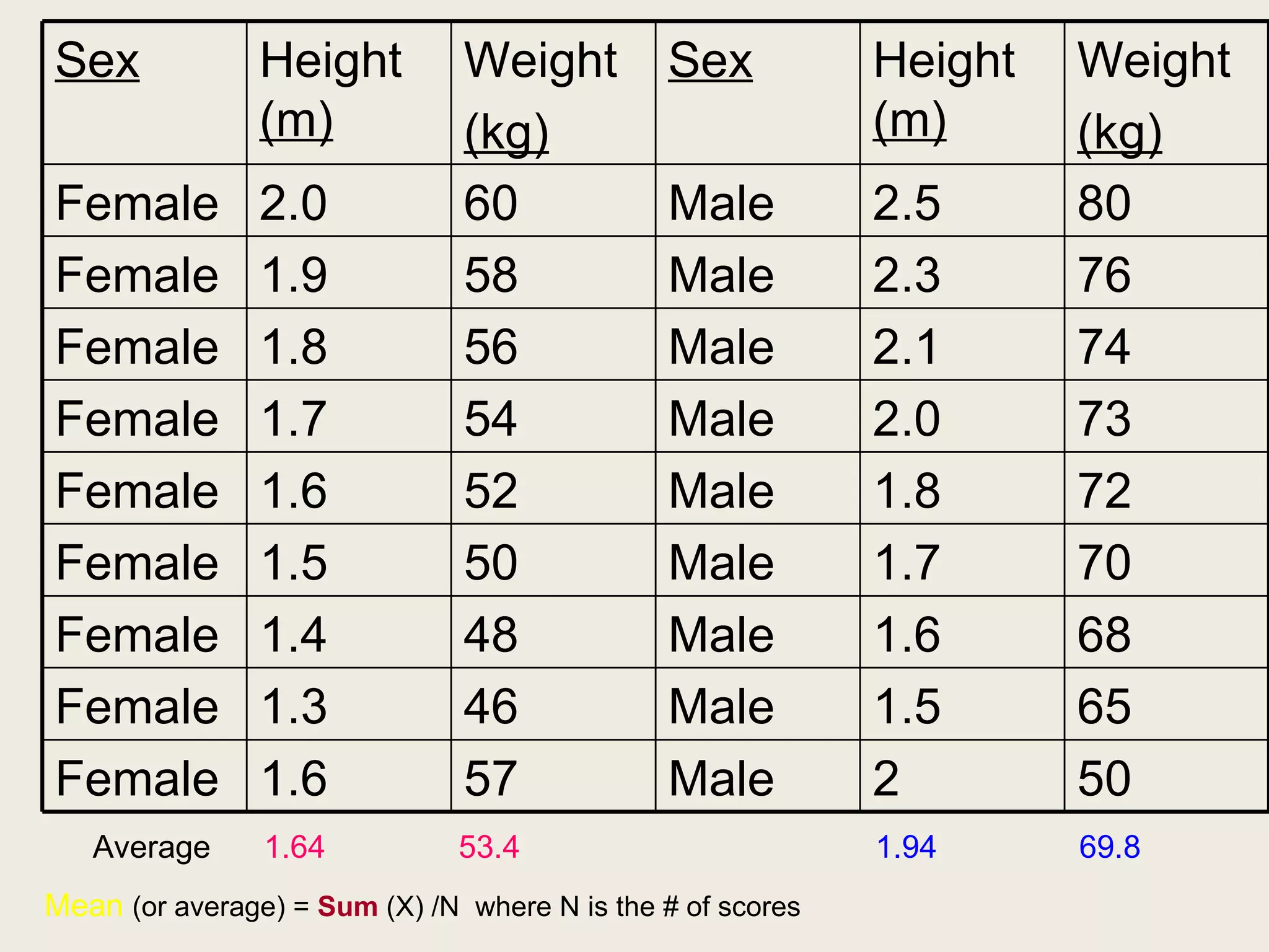
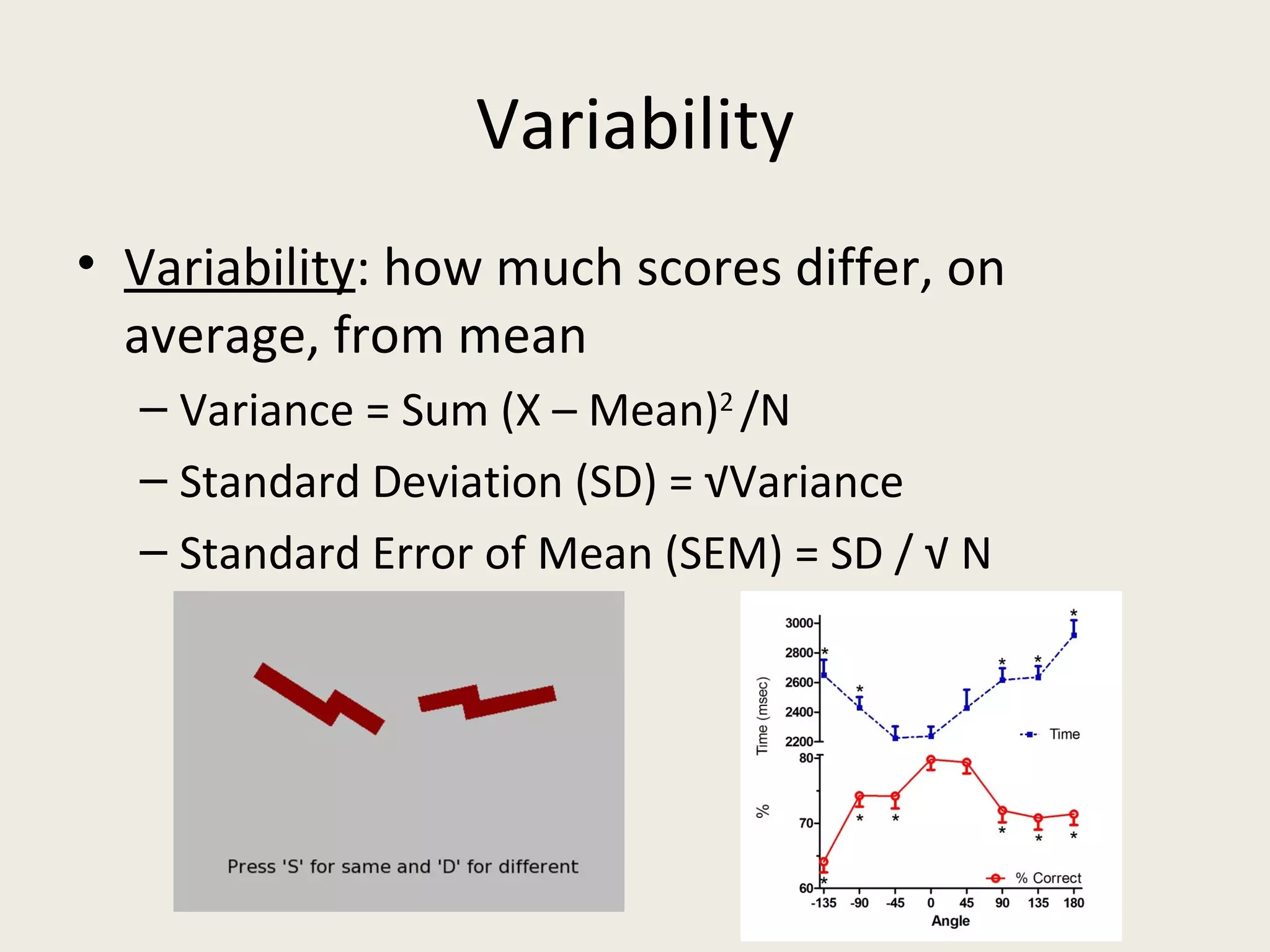
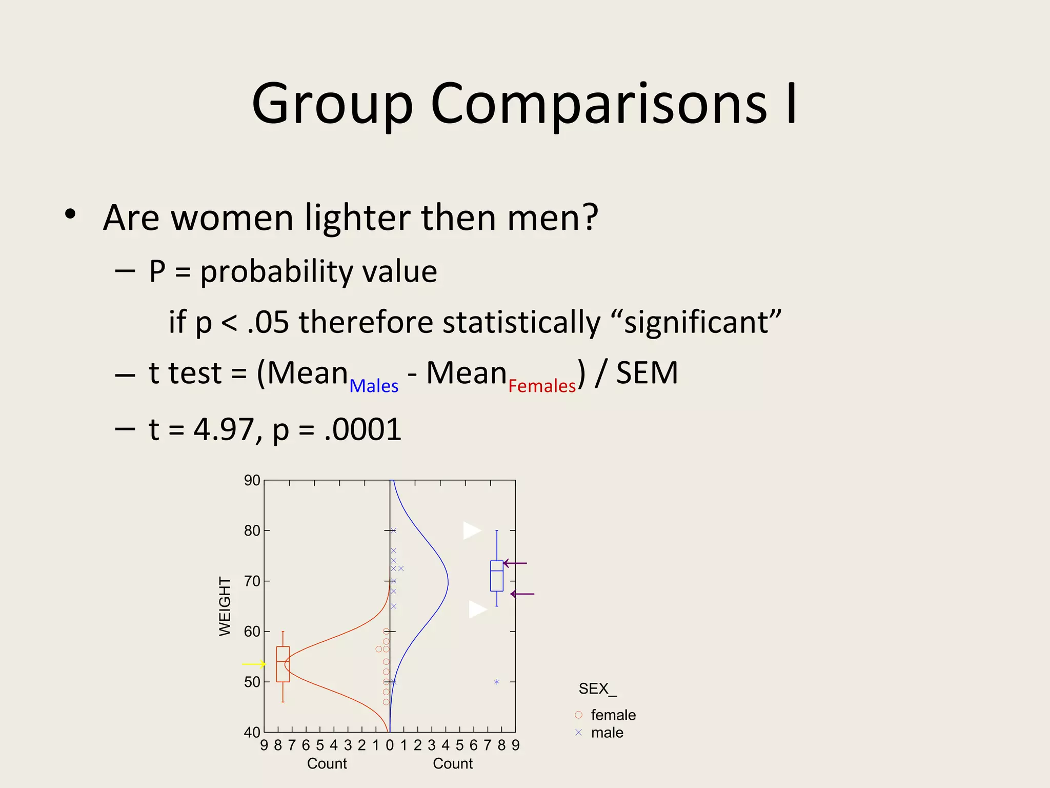
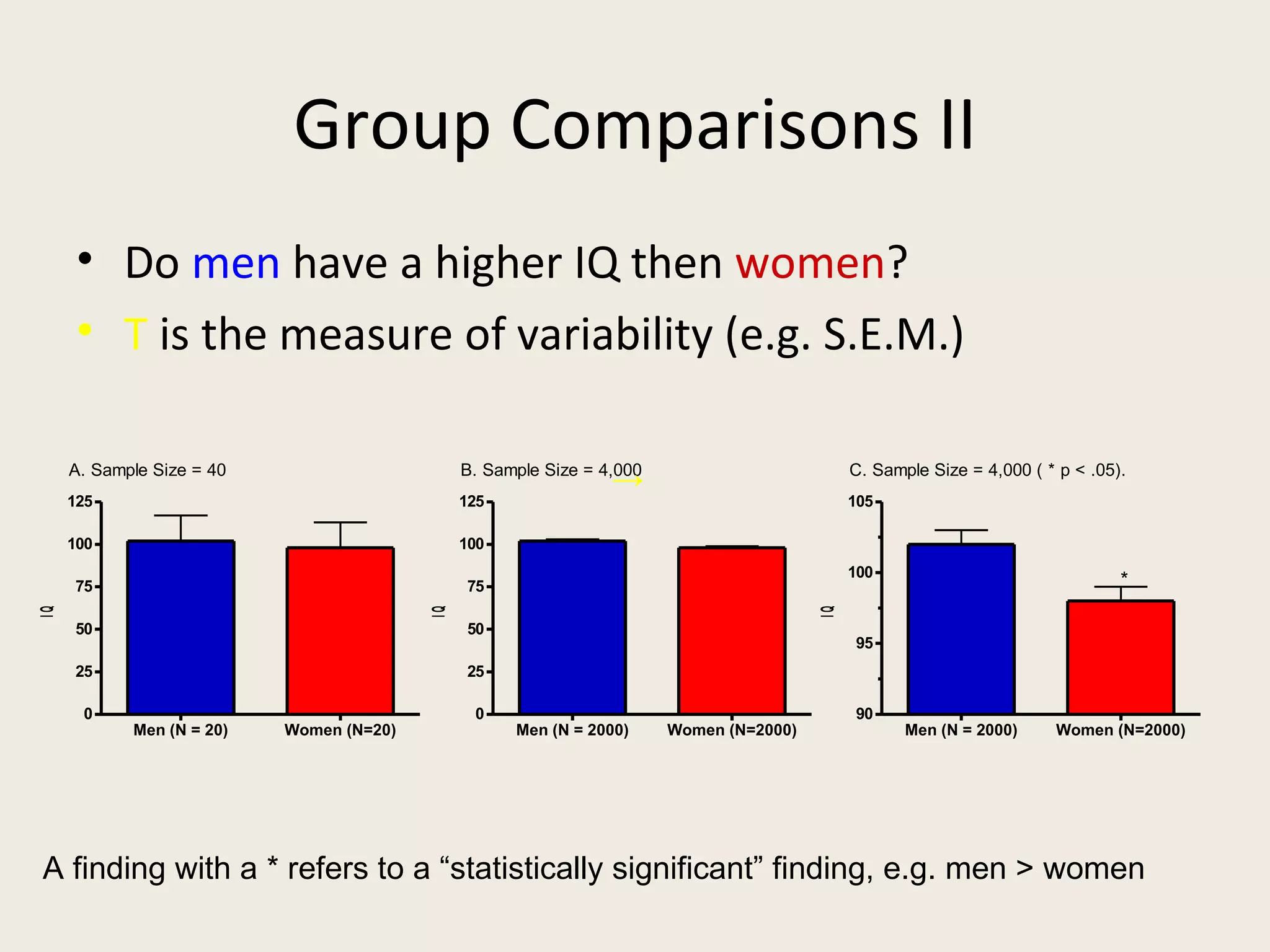
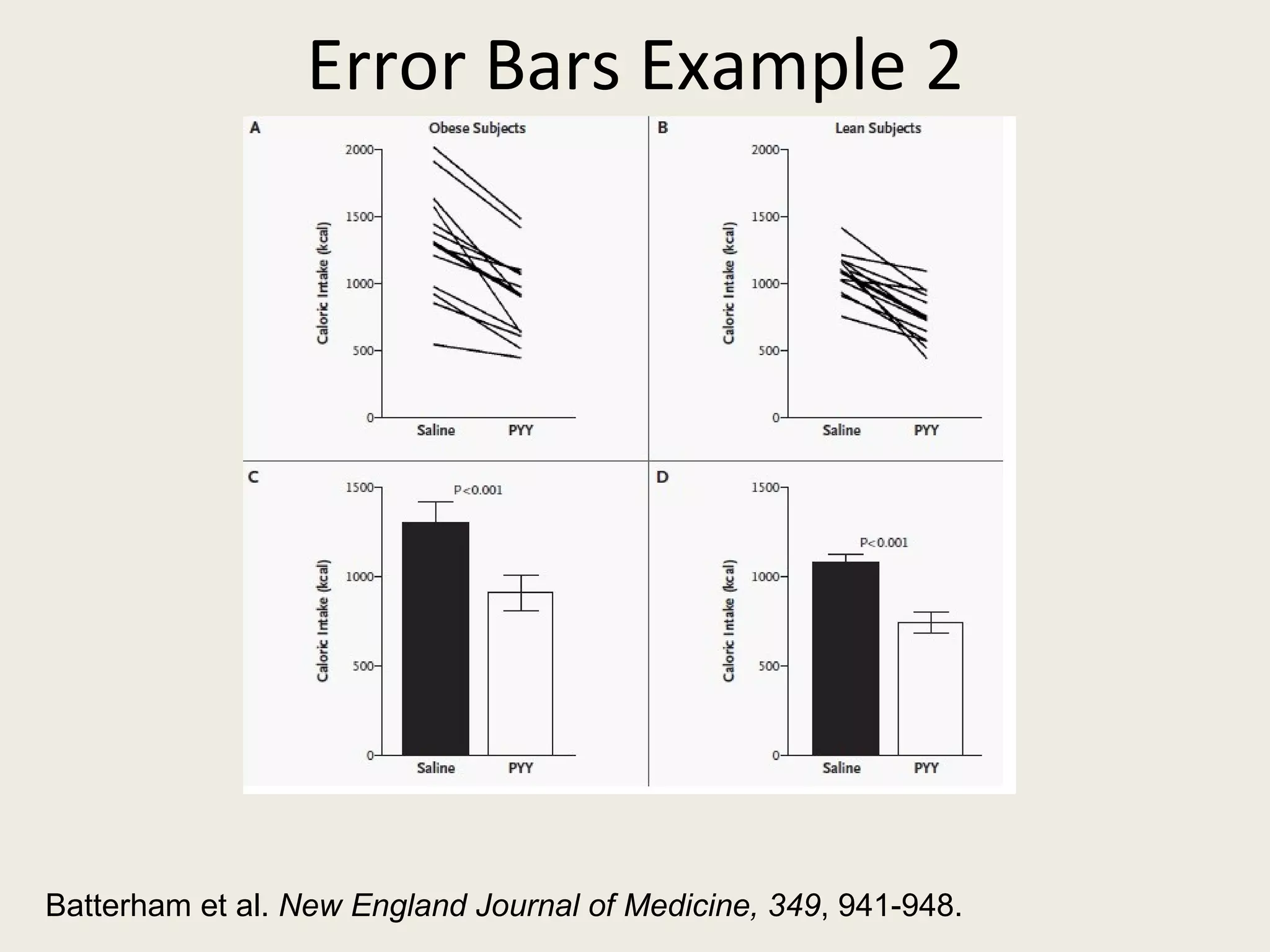
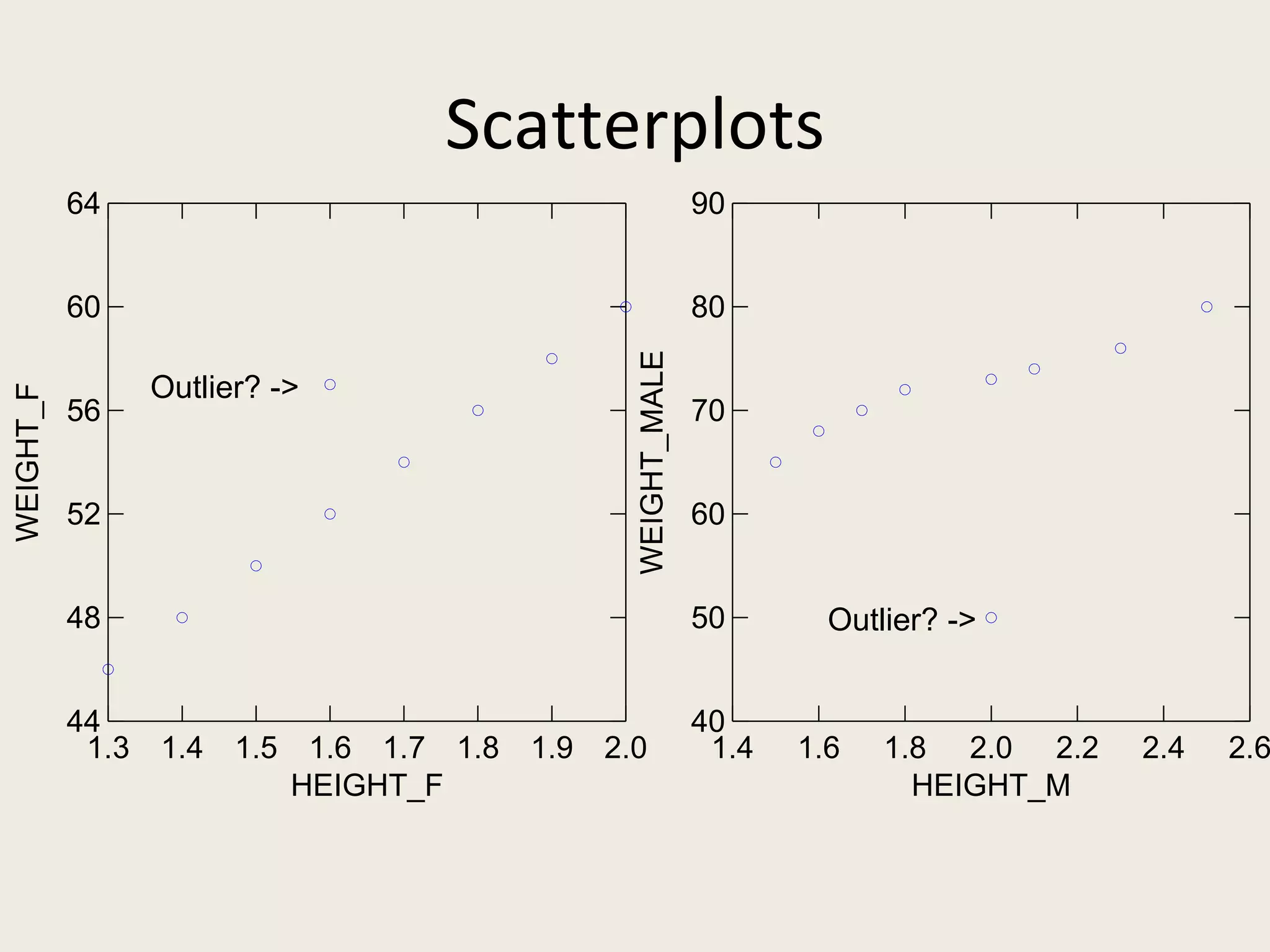
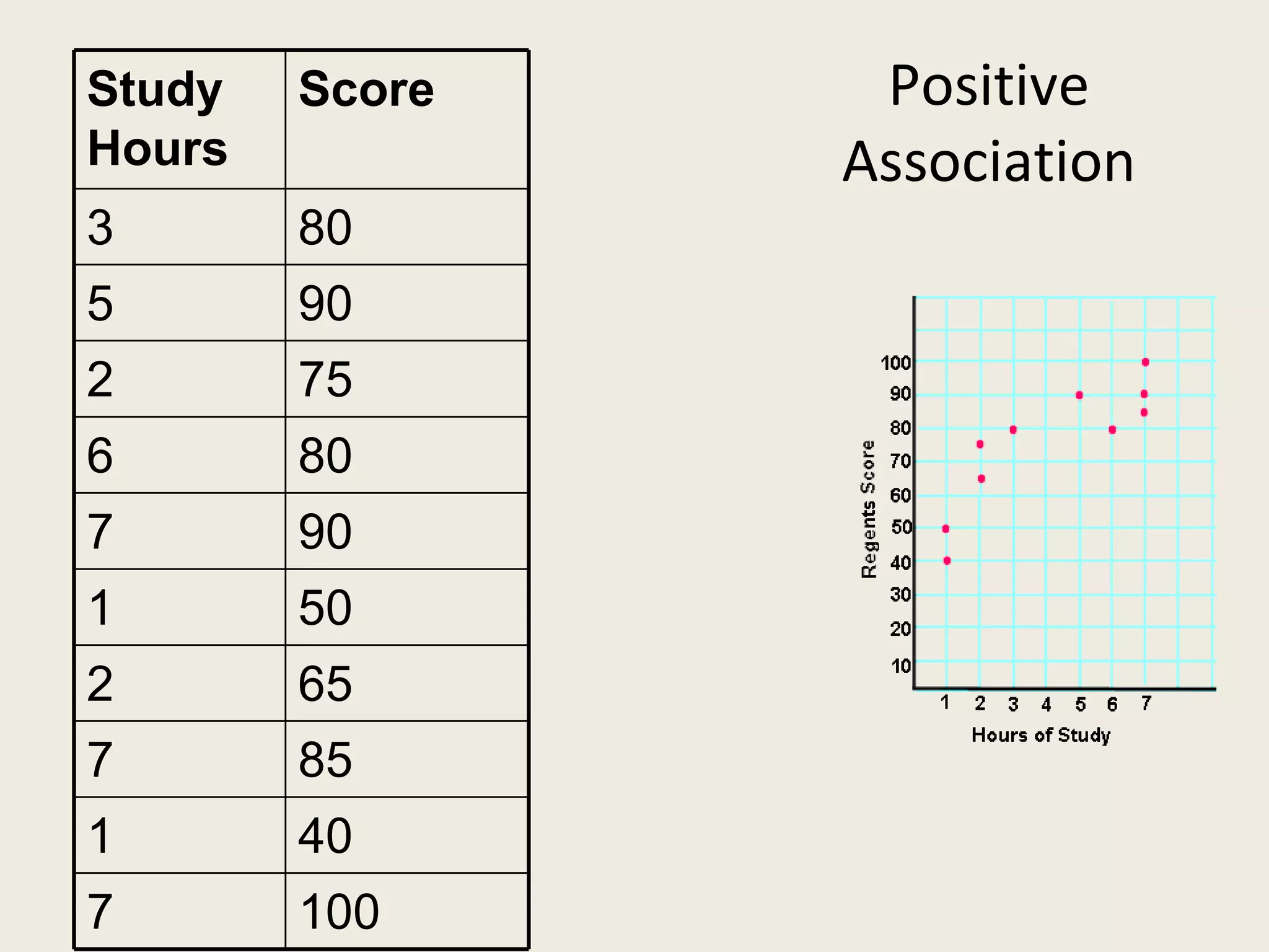
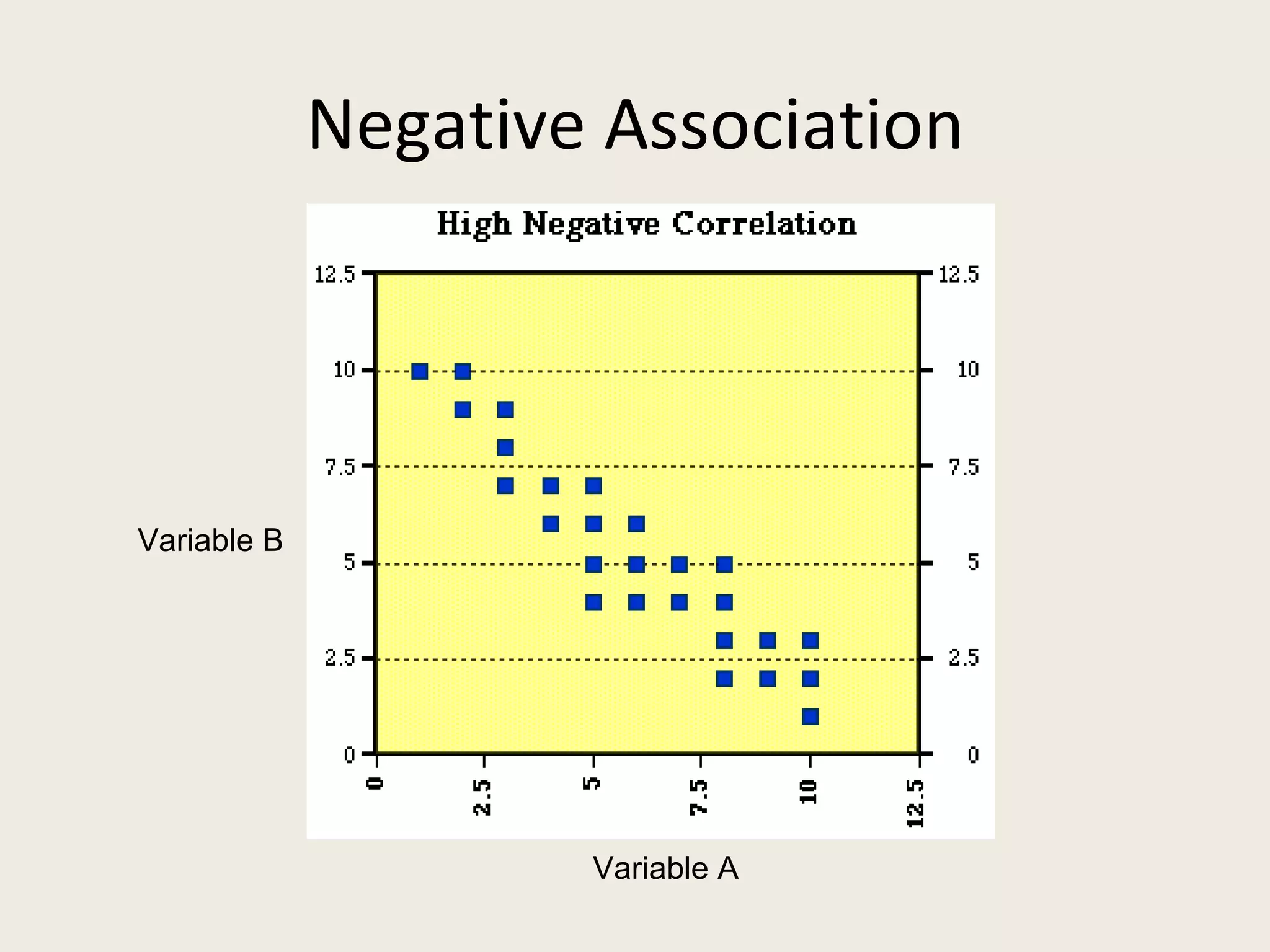
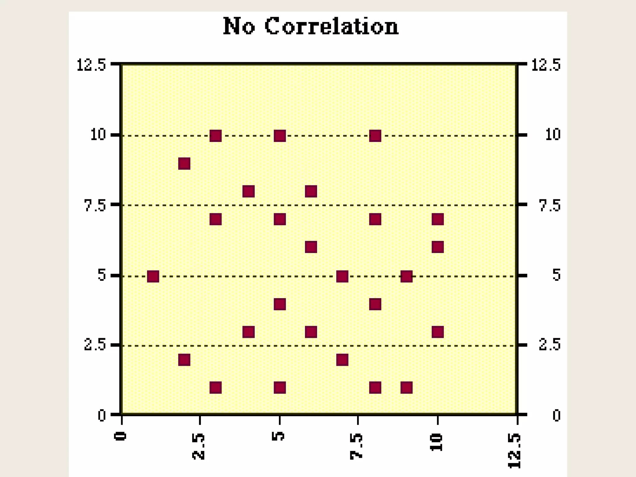
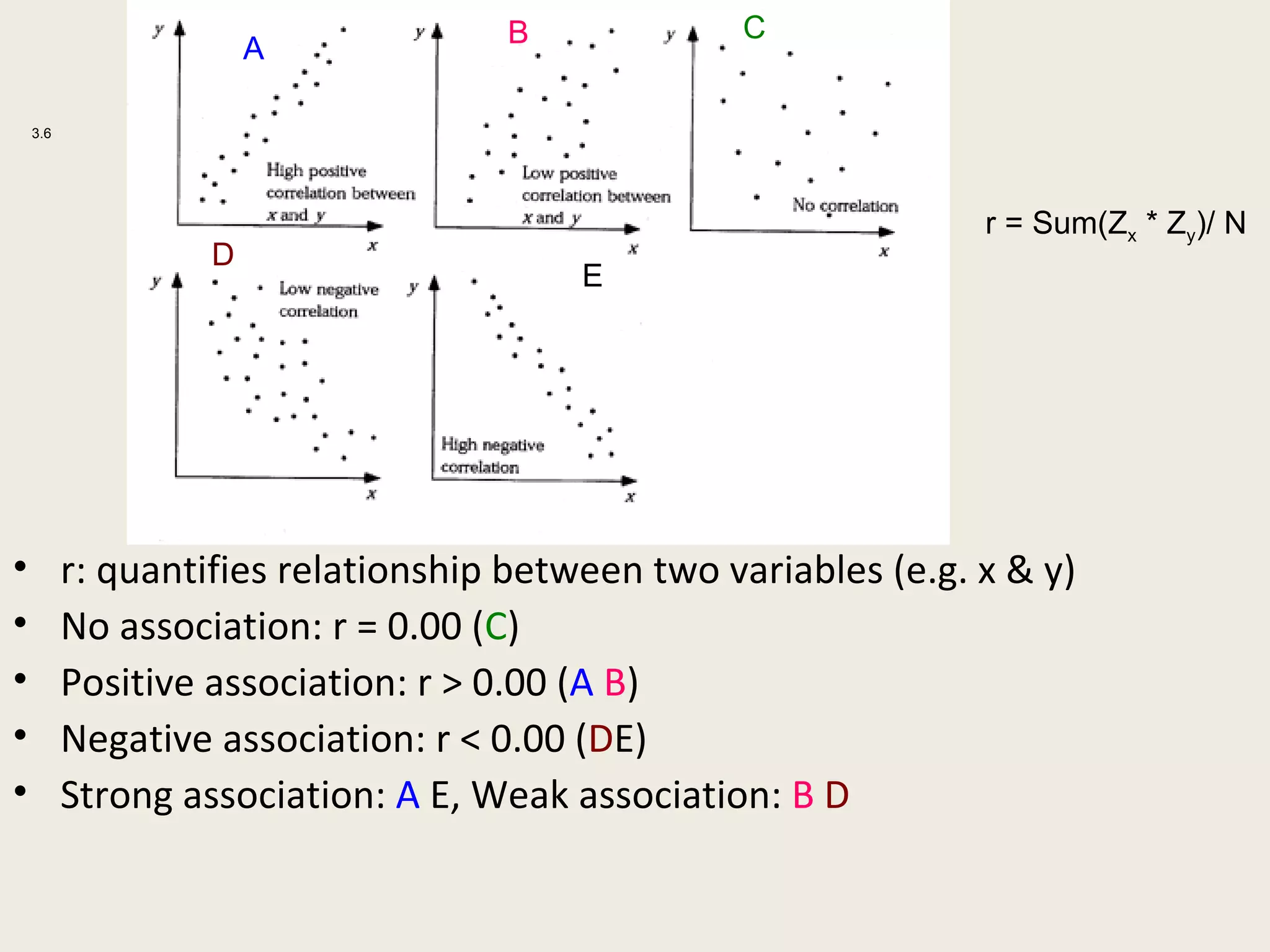
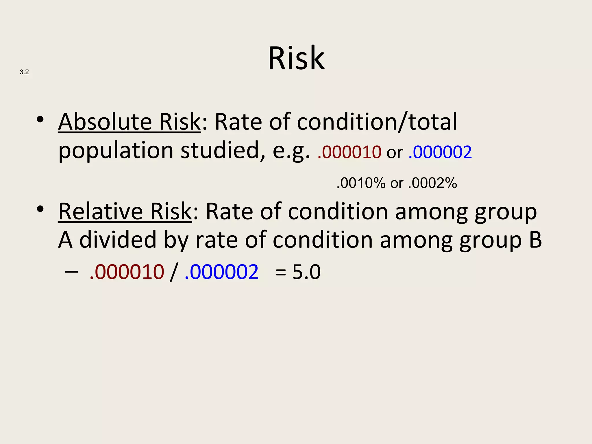
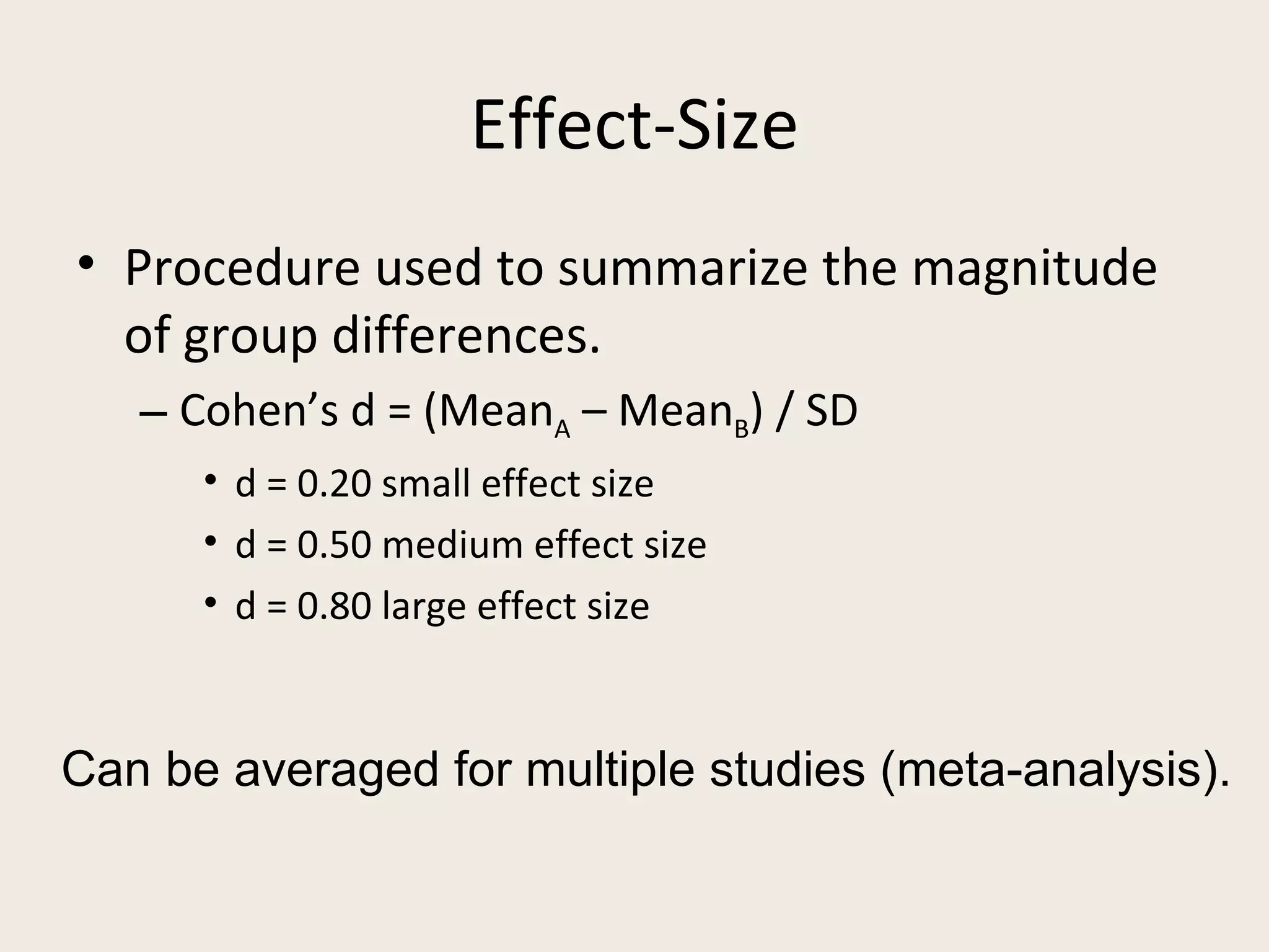
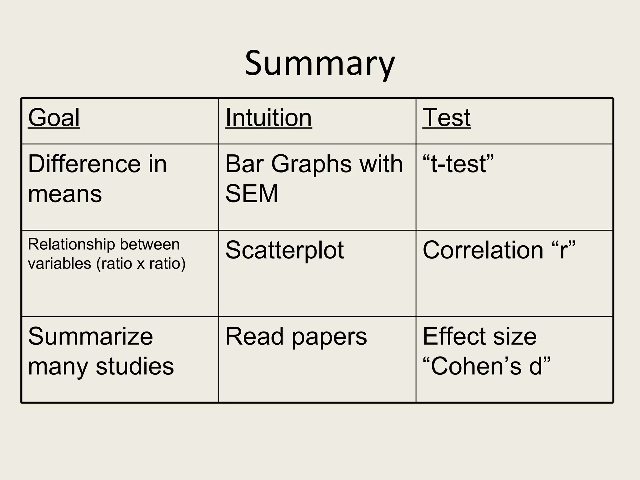
ψ
   Statistics

Brian J. Piper, Ph.D.
Mark Twain (?)
 • There are three types of lies, lies, damn lies,
   and statistics.


http://en.wikipedia.org/wiki/Lies,_damned_lies,_and_statistics
Goals
•   Levels of measurement
•   Group comparisons (t)
•   Association (scatterplot/r)
•   Effect-size (d)
)


               Levels of Measurement
• Nominal: categorical, example: sex
• Ratio: quantitative, example: age
• Ordinal: ranking, example: self-report
  –   Strongly disagree = 1
  –   Disagree = 2
  –   Neutral = 3
  –   Agree = 4
  –   Strongly agree = 5
  –   S.D.-------------------------------------------------------------------------------------------S.A.
What do these countries have in
             common?
• Liberia
• Burma
• United States
Metric System
Unit     Symbol     Factor
tera     T          1 x 10¹²
giga     G          1 x 10⁹
kilo     K          1 x 10³
---      --         1
centi    c          1 x 10⁻²
milli    m          1 x 10⁻³
micro    μ          1 x 10⁻⁶
Data
Sex      Height   Weight   Sex    Height   Weight
         (m)      (kg)            (m)      (kg)
Female   2.0      60       Male   2.5      80
Female   1.9      58       Male   2.3      76
Female   1.8      56       Male   2.1      74
Female   1.7      54       Male   2.0      73
Female   1.6      52       Male   1.8      72
Female   1.5      50       Male   1.7      70
Female   1.4      48       Male   1.6      68
Female   1.3      46       Male   1.5      65
Female   1.6      57       Male   2        50
Sex             Height         Weight         Sex           Height   Weight
                (m)            (kg)                         (m)      (kg)
Female          2.0            60             Male          2.5      80
Female          1.9            58             Male          2.3      76
Female          1.8            56             Male          2.1      74
Female          1.7            54             Male          2.0      73
Female          1.6            52             Male          1.8      72
Female          1.5            50             Male          1.7      70
Female          1.4            48             Male          1.6      68
Female          1.3            46             Male          1.5      65
Female          1.6            57             Male          2        50
   Average      1.64           53.4                         1.94     69.8
Mean (or average) = Sum (X) /N where N is the # of scores
Variability
• Variability: how much scores differ, on
  average, from mean
  – Variance = Sum (X – Mean)2 /N
  – Standard Deviation (SD) = √Variance
  – Standard Error of Mean (SEM) = SD / √ N
Group Comparisons I
• Are women lighter then men?
  – P = probability value
      if p < .05 therefore statistically “significant”
  – t test = (MeanMales - MeanFemales) / SEM
  – t = 4.97, p = .0001
                  90


                  80              ►
                                      ←
                  70
         WEIGHT


                                      ←
                                  ►
                  60

                  →
                  50                      SEX_
                                           female
                  40                       male
                    9876543210123456789
                       Count    Count
Group Comparisons II
      • Do men have a higher IQ then women?
      • T is the measure of variability (e.g. S.E.M.)

     A. Sample Size = 40                       B. Sample Size = 4,000                         C. Sample Size = 4,000 ( * p < .05).
                                                                 →
     125                                       125                                            105

     100                                       100
                                                                                              100
     75                                        75                                                                                *
IQ


                                          IQ


                                                                                         IQ
     50                                        50
                                                                                              95
     25                                        25

      0                                         0                                             90
            Men (N = 20)   Women (N=20)              Men (N = 2000)     Women (N=2000)               Men (N = 2000)     Women (N=2000)


A finding with a * refers to a “statistically significant” finding, e.g. men > women
Error Bars Example 2


Batterham et al. New England Journal of Medicine, 349, 941-948.
Scatterplots
           64                                                      90


           60                                                      80


                                                     WEIGHT_MALE
                  Outlier? ->
WEIGHT_F


           56                                                      70


           52                                                      60


           48                                                      50       Outlier? ->


           44                                                      40
            1.3   1.4   1.5    1.6 1.7 1.8   1.9   2.0              1.4   1.6   1.8 2.0 2.2   2.4   2.6
                              HEIGHT_F                                            HEIGHT_M
Study   Score    Positive
Hours           Association
3       80
5       90
2       75
6       80
7       90
1       50
2       65
7       85
1       40
7       100
Negative Association


Variable B


                     Variable A
3.1
                Standardized “Z” Scores
      •   Z is a #
      •   Z = 0 therefore average
      •   Z > 0 therefore above average
      •   Z < 0 therefore below average

      • Z = (X – Mean) / SD
      • Z = (600 – 500) / 100
            = 1.0
B             C
                       A

    3.6


                                                                 r = Sum(Zx * Zy)/ N
                   D
                                         E


•         r: quantifies relationship between two variables (e.g. x & y)
•         No association: r = 0.00 (C)
•         Positive association: r > 0.00 (A B)
•         Negative association: r < 0.00 (DE)
•         Strong association: A E, Weak association: B D
Probability
                            Eyes                                  Eyes
                                          Probability
         Frequency   Blue      Brown                    Blue        Brown


                                                        .000002     .000010
         +           2         10         +


Brain
Cancer                                                  .999998     .99999
         -           999,998 999,990      -
3.2
                             Risk
      • Absolute Risk: Rate of condition/total
        population studied, e.g. .000010 or .000002
                                     .0010% or .0002%

      • Relative Risk: Rate of condition among group
        A divided by rate of condition among group B
         – .000010 / .000002 = 5.0
Effect-Size
• Procedure used to summarize the magnitude
  of group differences.
   – Cohen’s d = (MeanA – MeanB) / SD
      • d = 0.20 small effect size
      • d = 0.50 medium effect size
      • d = 0.80 large effect size


Can be averaged for multiple studies (meta-analysis).
D.A.R.E.
        • Founded in 1983 by Daryl Gates
        • Police officers give lectures to middle school
        • Found in 80% of U.S. school districts, 54
          nations
        • Cohen’s d = (Mean – Mean )/ SD       D.A.R.E.          Control   pop


                       d = 0.30 small, 0.50 medium, 0.70 large


http://www.dare.com/home/default.asp
Does D.A.R.E work?


Ennett S.T. (1994). American Journal of Public Health, 84, 1394-1401.
Summary
Goal                        Intuition        Test
Difference in               Bar Graphs with “t-test”
means                       SEM
Relationship between
variables (ratio x ratio)
                            Scatterplot      Correlation “r”


Summarize                   Read papers      Effect size
many studies                                 “Cohen’s d”

Research Methods: Statistics

  • 1.
    ψ Statistics Brian J. Piper, Ph.D.
  • 2.
    Mark Twain (?) • There are three types of lies, lies, damn lies, and statistics. http://en.wikipedia.org/wiki/Lies,_damned_lies,_and_statistics
  • 3.
    Goals • Levels of measurement • Group comparisons (t) • Association (scatterplot/r) • Effect-size (d)
  • 4.
    ) Levels of Measurement • Nominal: categorical, example: sex • Ratio: quantitative, example: age • Ordinal: ranking, example: self-report – Strongly disagree = 1 – Disagree = 2 – Neutral = 3 – Agree = 4 – Strongly agree = 5 – S.D.-------------------------------------------------------------------------------------------S.A.
  • 5.
    What do thesecountries have in common? • Liberia • Burma • United States
  • 6.
    Metric System Unit Symbol Factor tera T 1 x 10¹² giga G 1 x 10⁹ kilo K 1 x 10³ --- -- 1 centi c 1 x 10⁻² milli m 1 x 10⁻³ micro μ 1 x 10⁻⁶
  • 7.
    Data Sex Height Weight Sex Height Weight (m) (kg) (m) (kg) Female 2.0 60 Male 2.5 80 Female 1.9 58 Male 2.3 76 Female 1.8 56 Male 2.1 74 Female 1.7 54 Male 2.0 73 Female 1.6 52 Male 1.8 72 Female 1.5 50 Male 1.7 70 Female 1.4 48 Male 1.6 68 Female 1.3 46 Male 1.5 65 Female 1.6 57 Male 2 50
  • 8.
    Sex Height Weight Sex Height Weight (m) (kg) (m) (kg) Female 2.0 60 Male 2.5 80 Female 1.9 58 Male 2.3 76 Female 1.8 56 Male 2.1 74 Female 1.7 54 Male 2.0 73 Female 1.6 52 Male 1.8 72 Female 1.5 50 Male 1.7 70 Female 1.4 48 Male 1.6 68 Female 1.3 46 Male 1.5 65 Female 1.6 57 Male 2 50 Average 1.64 53.4 1.94 69.8 Mean (or average) = Sum (X) /N where N is the # of scores
  • 9.
    Variability • Variability: howmuch scores differ, on average, from mean – Variance = Sum (X – Mean)2 /N – Standard Deviation (SD) = √Variance – Standard Error of Mean (SEM) = SD / √ N
  • 10.
    Group Comparisons I •Are women lighter then men? – P = probability value if p < .05 therefore statistically “significant” – t test = (MeanMales - MeanFemales) / SEM – t = 4.97, p = .0001 90 80 ► ← 70 WEIGHT ← ► 60 → 50 SEX_ female 40 male 9876543210123456789 Count Count
  • 11.
    Group Comparisons II • Do men have a higher IQ then women? • T is the measure of variability (e.g. S.E.M.) A. Sample Size = 40 B. Sample Size = 4,000 C. Sample Size = 4,000 ( * p < .05). → 125 125 105 100 100 100 75 75 * IQ IQ IQ 50 50 95 25 25 0 0 90 Men (N = 20) Women (N=20) Men (N = 2000) Women (N=2000) Men (N = 2000) Women (N=2000) A finding with a * refers to a “statistically significant” finding, e.g. men > women
  • 12.
    Error Bars Example2 Batterham et al. New England Journal of Medicine, 349, 941-948.
  • 13.
    Scatterplots 64 90 60 80 WEIGHT_MALE Outlier? -> WEIGHT_F 56 70 52 60 48 50 Outlier? -> 44 40 1.3 1.4 1.5 1.6 1.7 1.8 1.9 2.0 1.4 1.6 1.8 2.0 2.2 2.4 2.6 HEIGHT_F HEIGHT_M
  • 14.
    Study Score Positive Hours Association 3 80 5 90 2 75 6 80 7 90 1 50 2 65 7 85 1 40 7 100
  • 15.
  • 17.
    3.1 Standardized “Z” Scores • Z is a # • Z = 0 therefore average • Z > 0 therefore above average • Z < 0 therefore below average • Z = (X – Mean) / SD • Z = (600 – 500) / 100 = 1.0
  • 18.
    B C A 3.6 r = Sum(Zx * Zy)/ N D E • r: quantifies relationship between two variables (e.g. x & y) • No association: r = 0.00 (C) • Positive association: r > 0.00 (A B) • Negative association: r < 0.00 (DE) • Strong association: A E, Weak association: B D
  • 19.
    Probability Eyes Eyes Probability Frequency Blue Brown Blue Brown .000002 .000010 + 2 10 + Brain Cancer .999998 .99999 - 999,998 999,990 -
  • 20.
    3.2 Risk • Absolute Risk: Rate of condition/total population studied, e.g. .000010 or .000002 .0010% or .0002% • Relative Risk: Rate of condition among group A divided by rate of condition among group B – .000010 / .000002 = 5.0
  • 21.
    Effect-Size • Procedure usedto summarize the magnitude of group differences. – Cohen’s d = (MeanA – MeanB) / SD • d = 0.20 small effect size • d = 0.50 medium effect size • d = 0.80 large effect size Can be averaged for multiple studies (meta-analysis).
  • 22.
    D.A.R.E. • Founded in 1983 by Daryl Gates • Police officers give lectures to middle school • Found in 80% of U.S. school districts, 54 nations • Cohen’s d = (Mean – Mean )/ SD D.A.R.E. Control pop d = 0.30 small, 0.50 medium, 0.70 large http://www.dare.com/home/default.asp
  • 23.
    Does D.A.R.E work? EnnettS.T. (1994). American Journal of Public Health, 84, 1394-1401.
  • 24.
    Summary Goal Intuition Test Difference in Bar Graphs with “t-test” means SEM Relationship between variables (ratio x ratio) Scatterplot Correlation “r” Summarize Read papers Effect size many studies “Cohen’s d”