This document outlines an experiment conducted for a marketing research class. It discusses different types of experimental designs, including between-subjects and within-subjects designs. It also covers the trade-offs between field and lab experiments. Finally, it provides an overview of statistical analysis techniques like ANOVA and regression that can be used to analyze experimental data, including an example experiment involving different advertising themes and price levels.

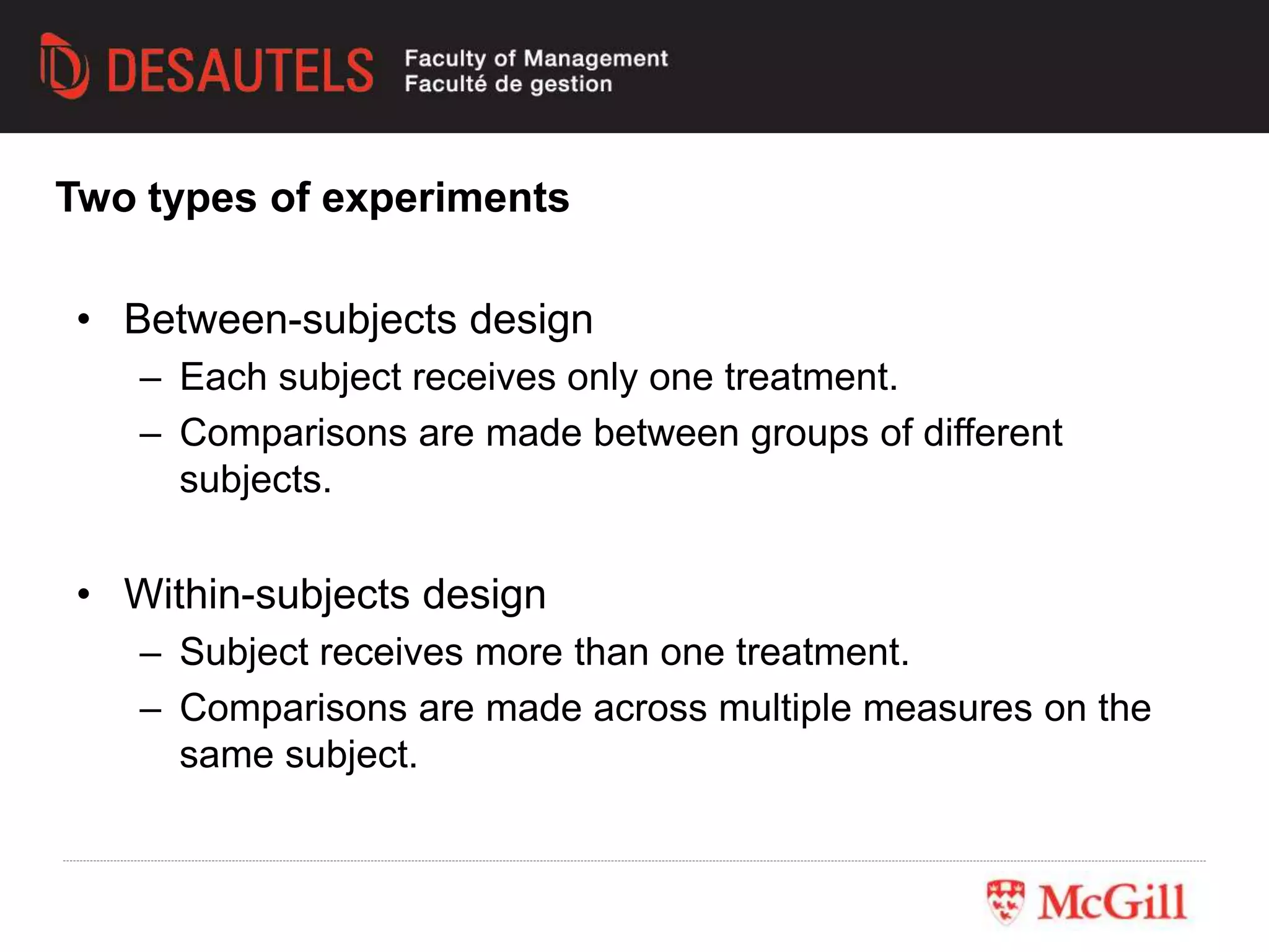
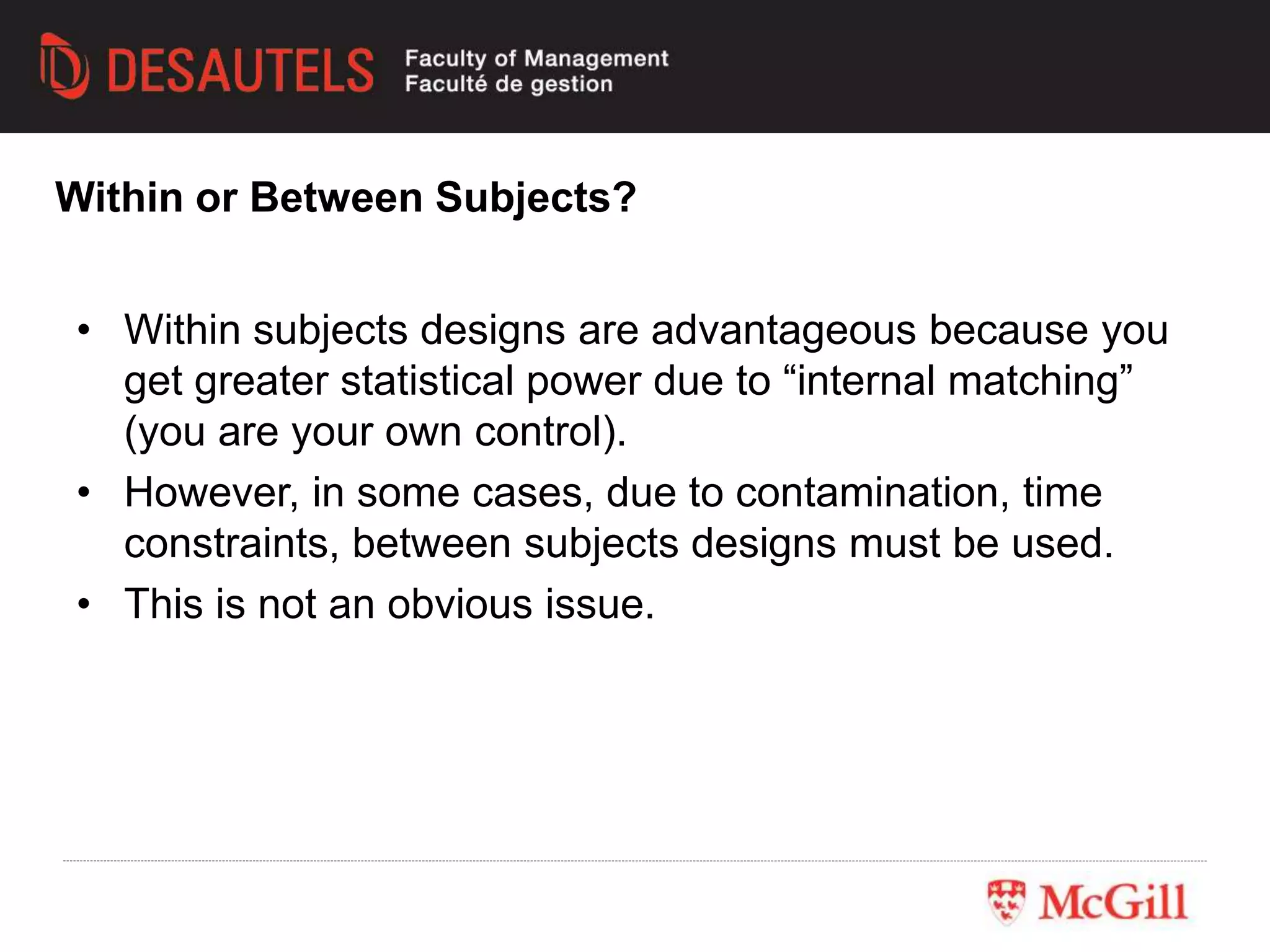
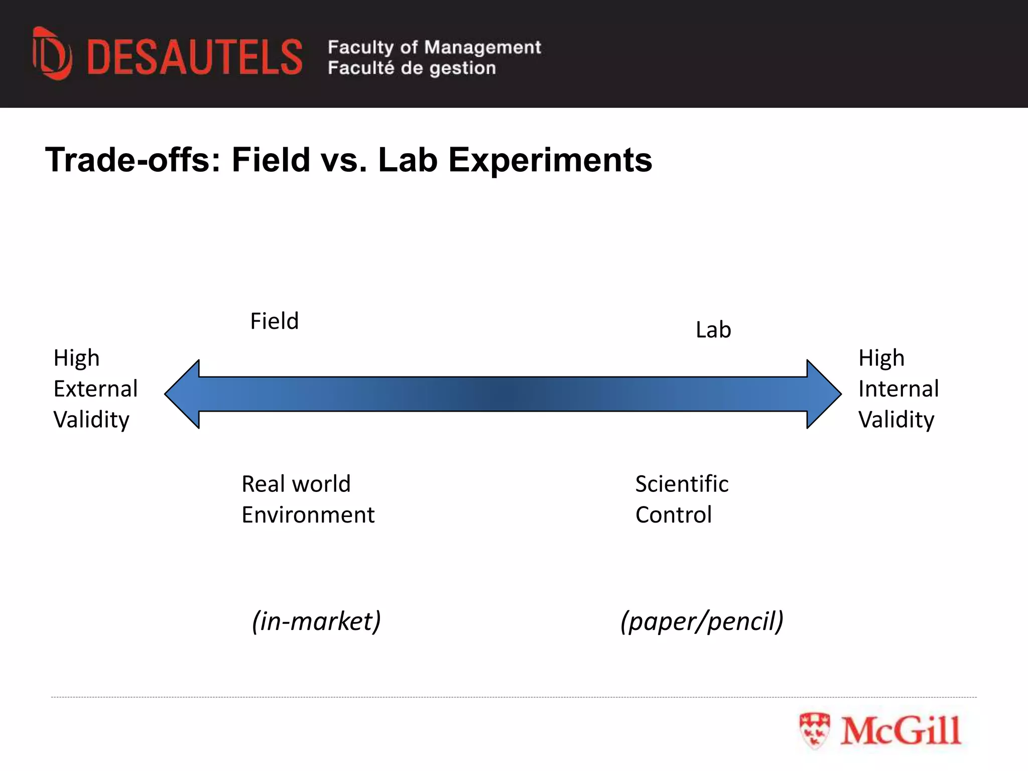
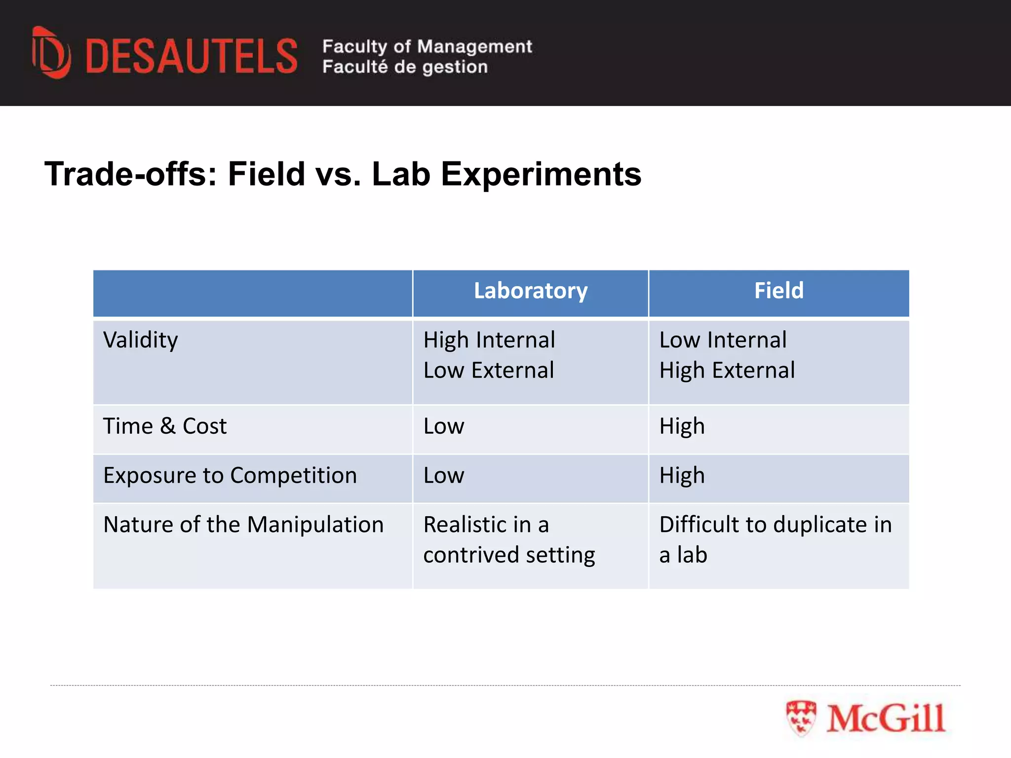
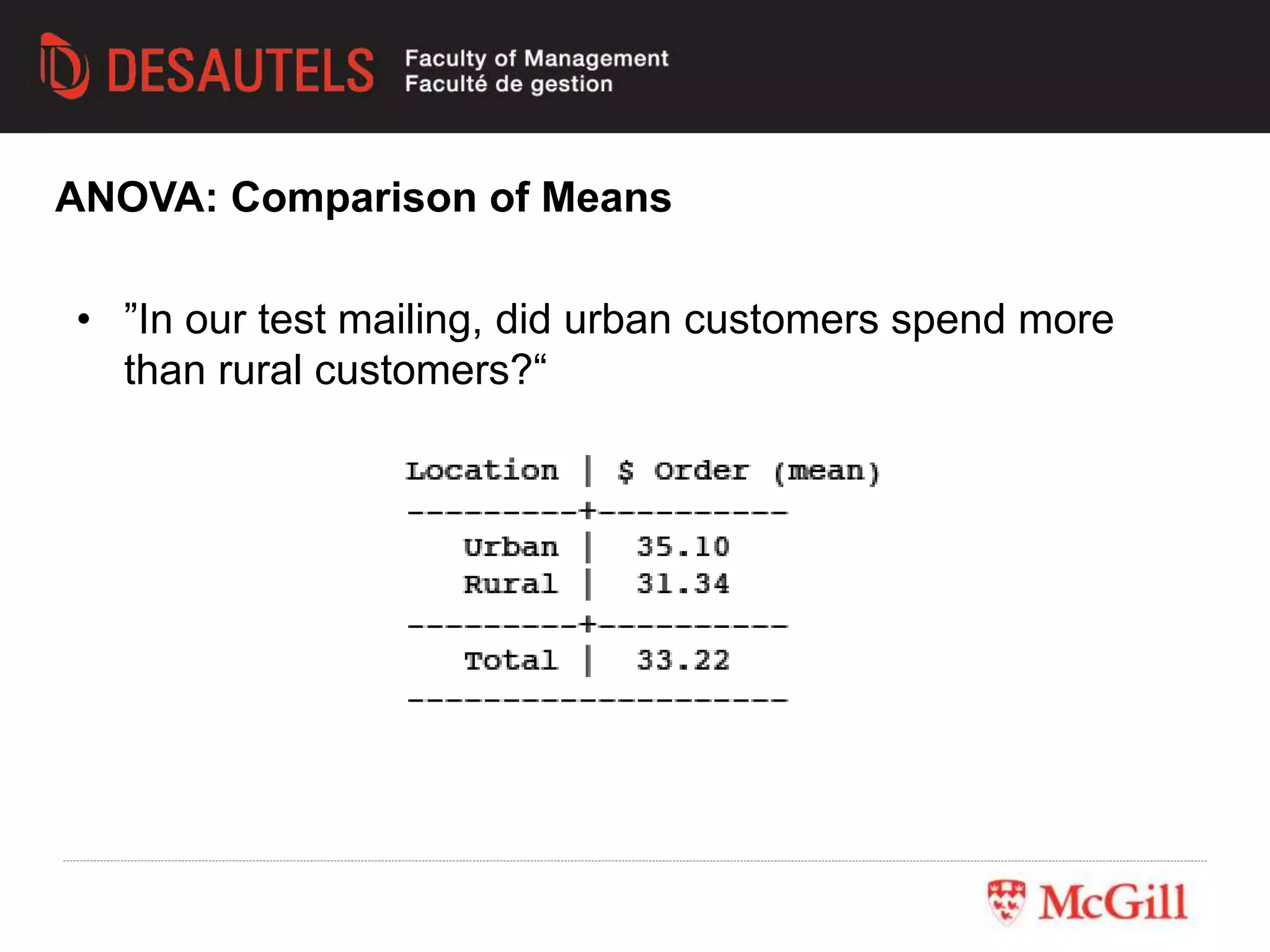
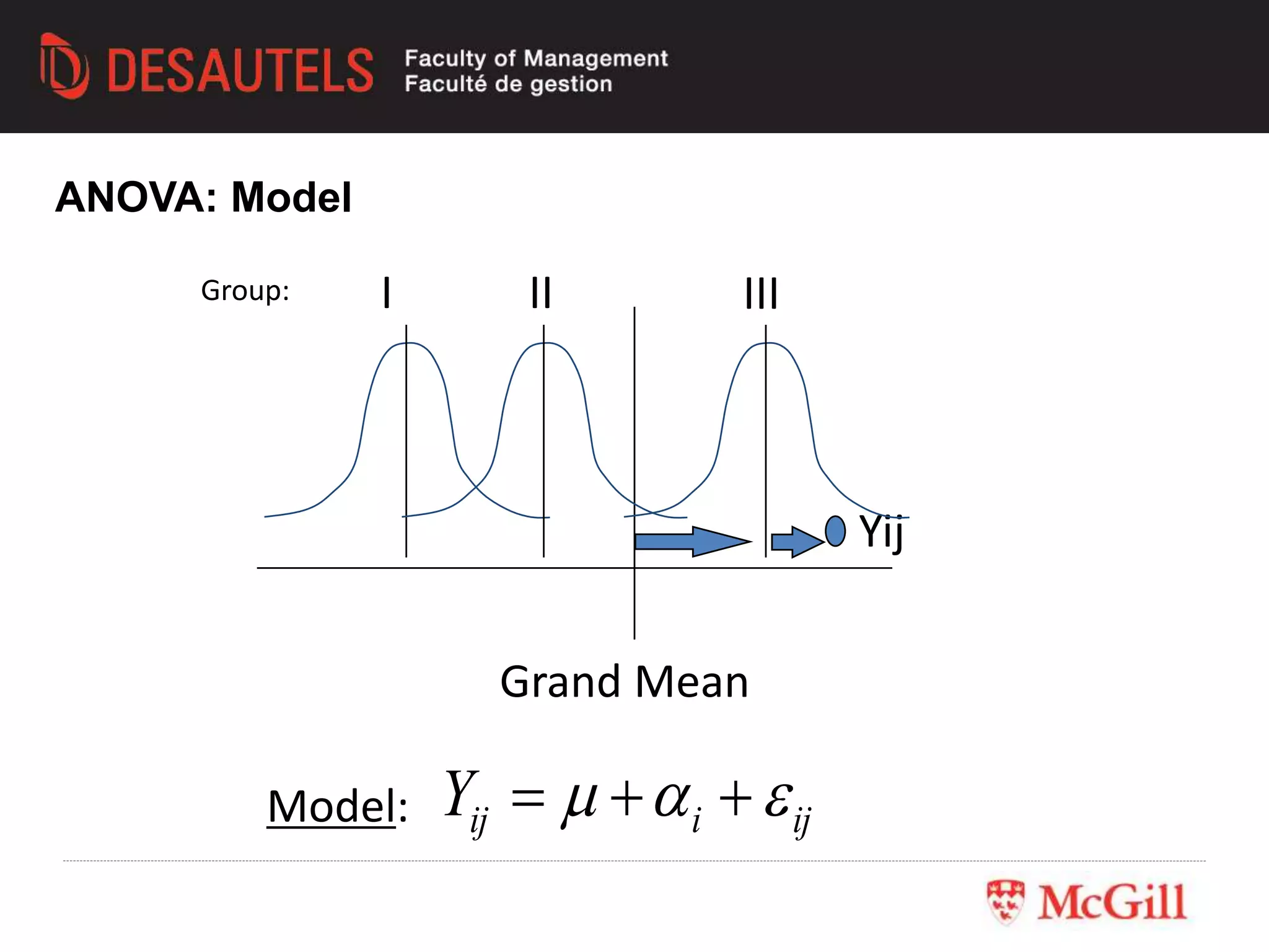
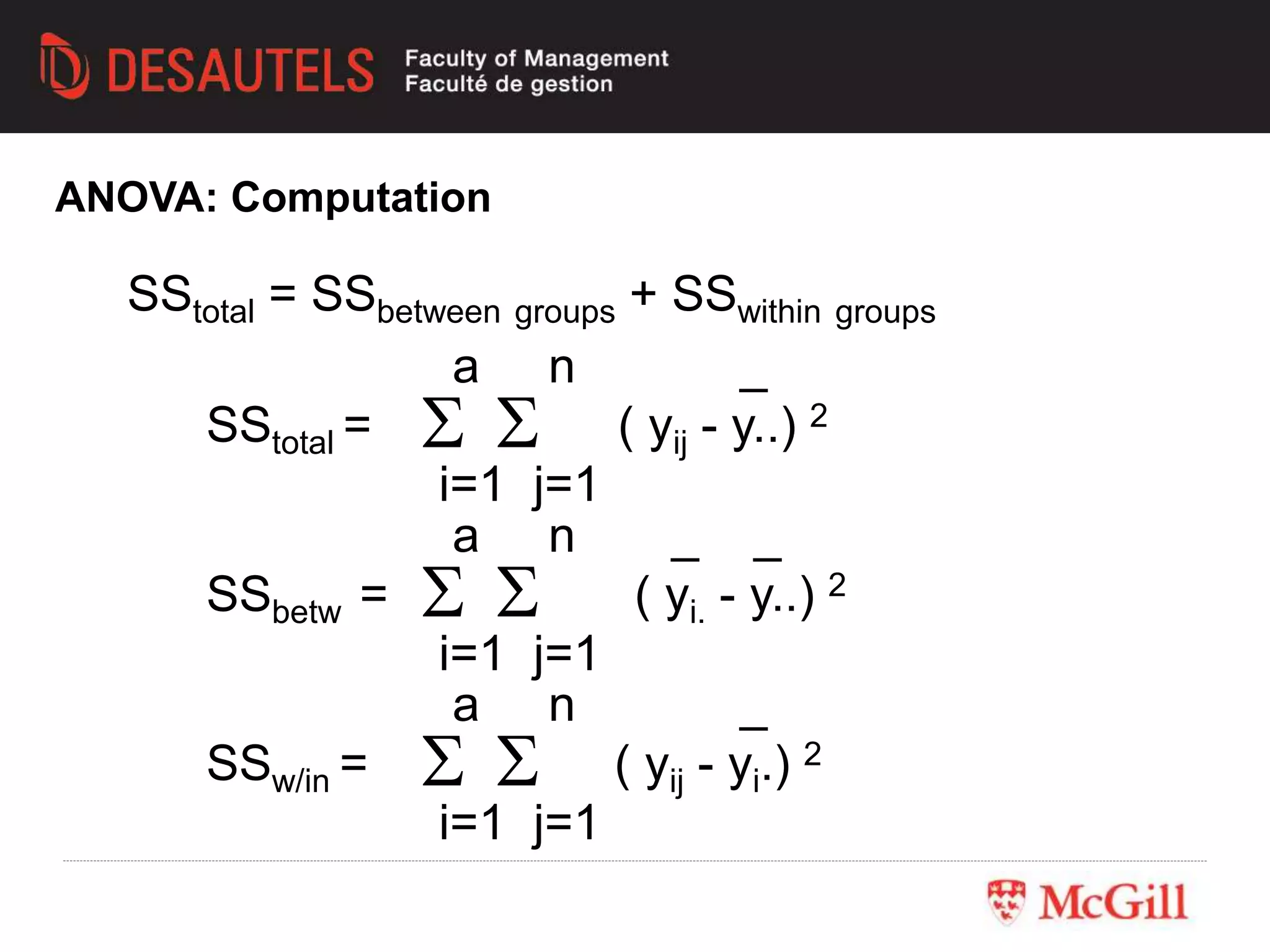
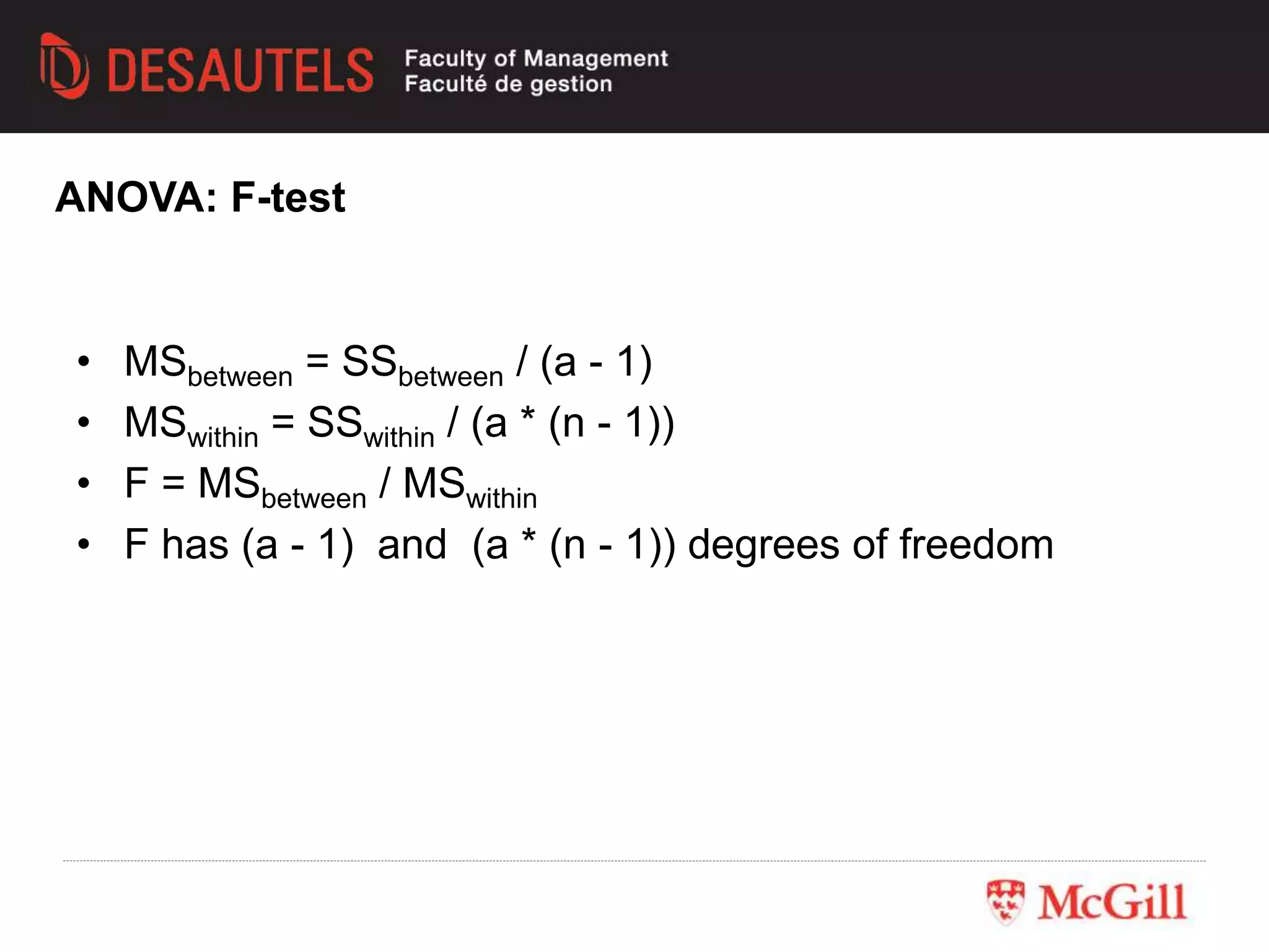
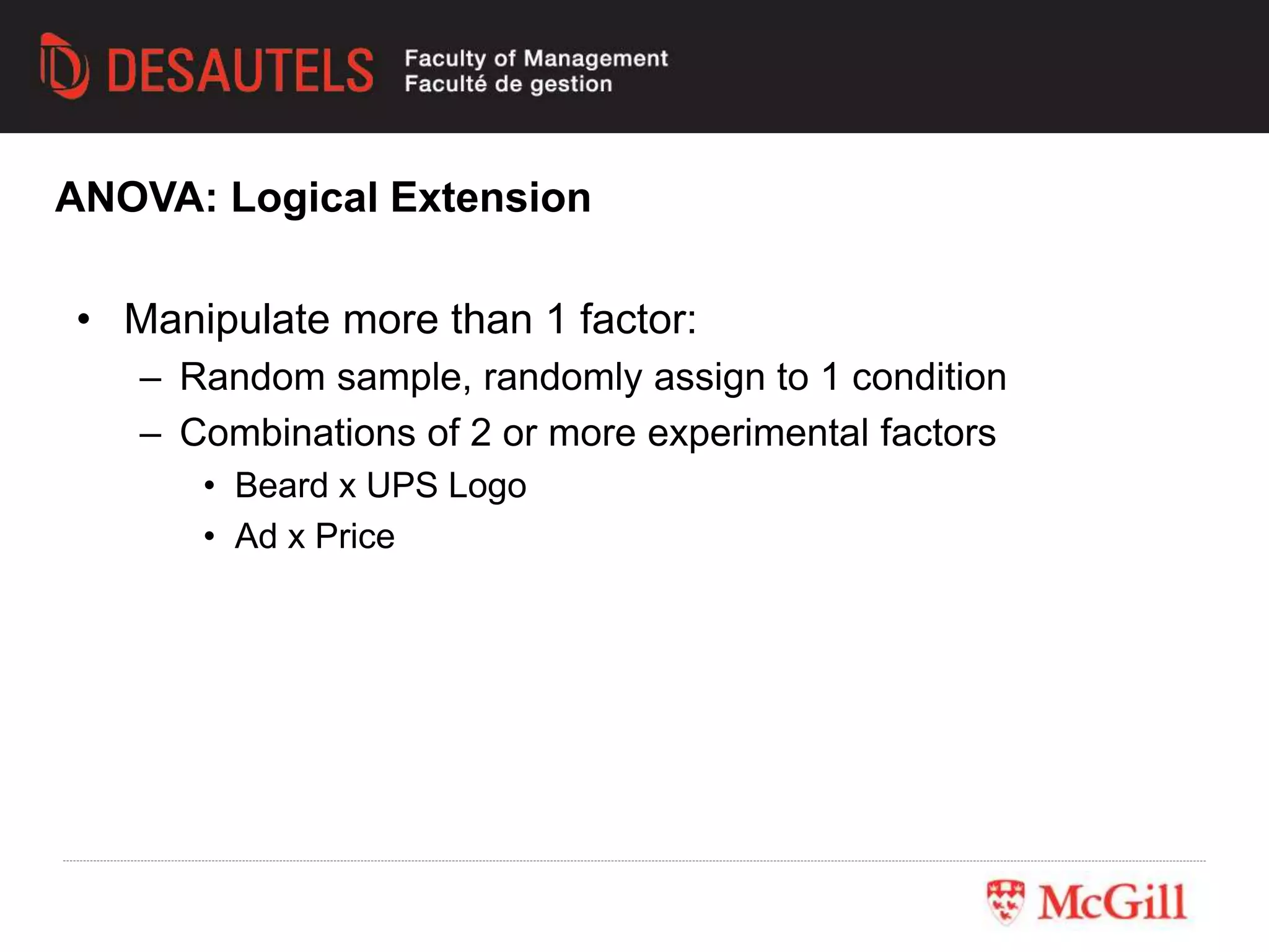
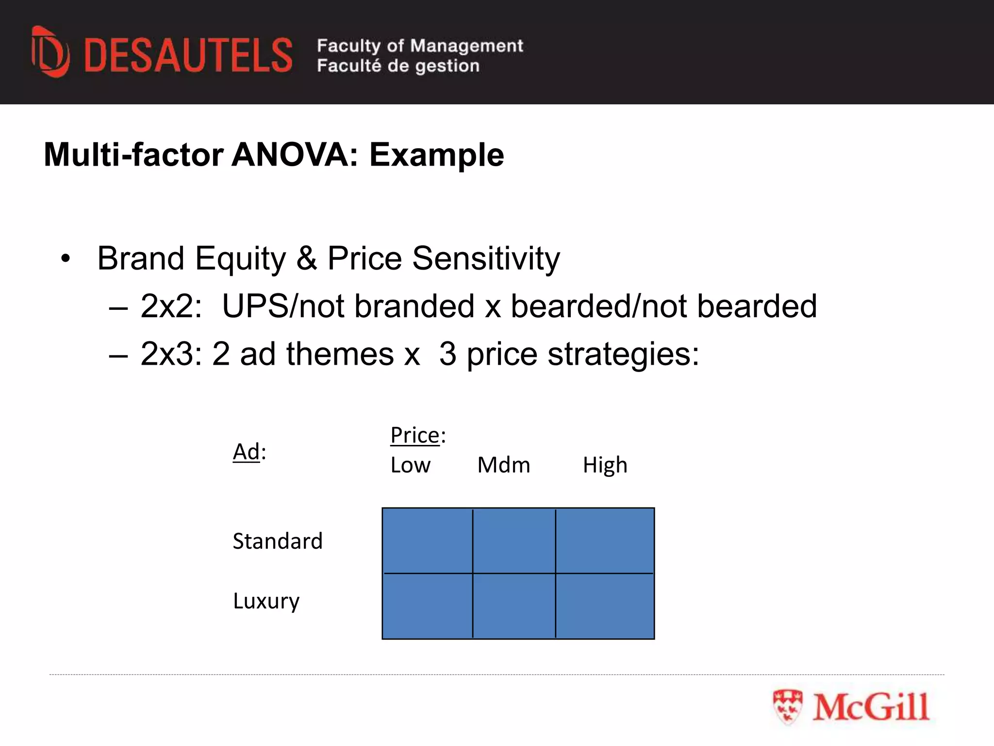
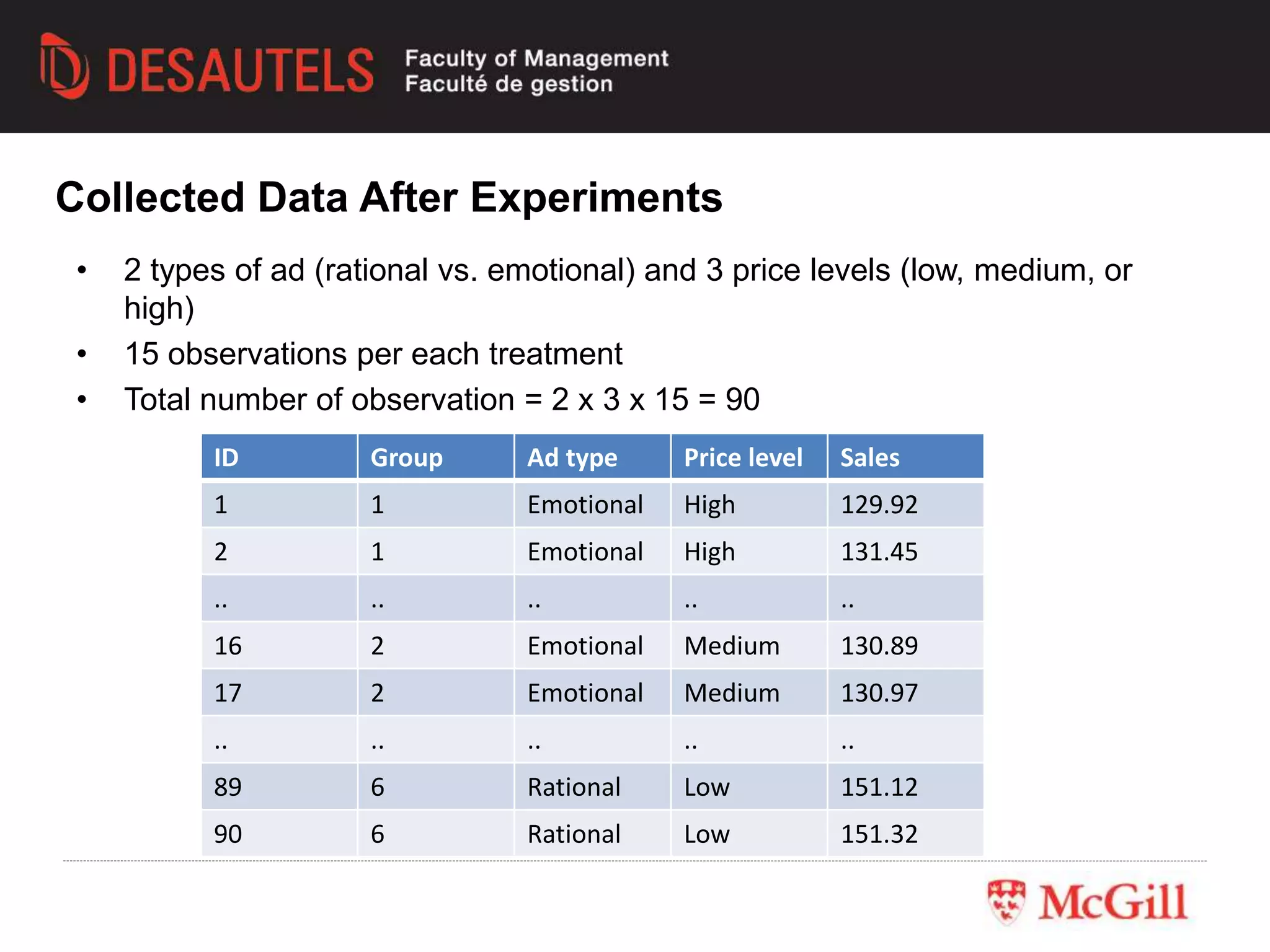
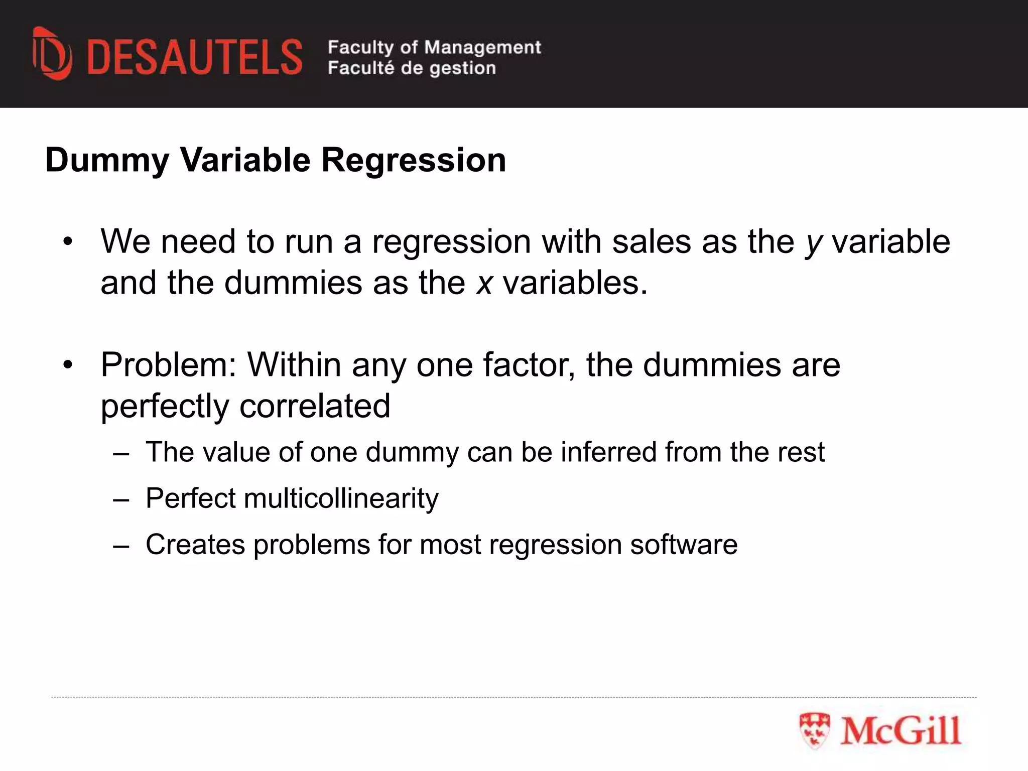
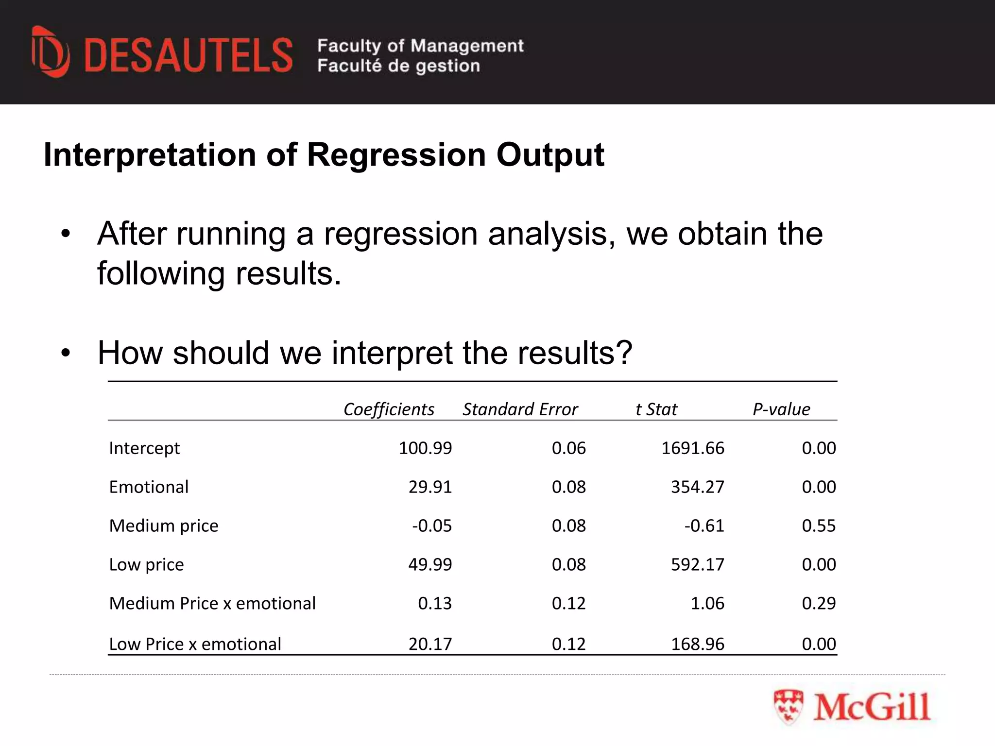
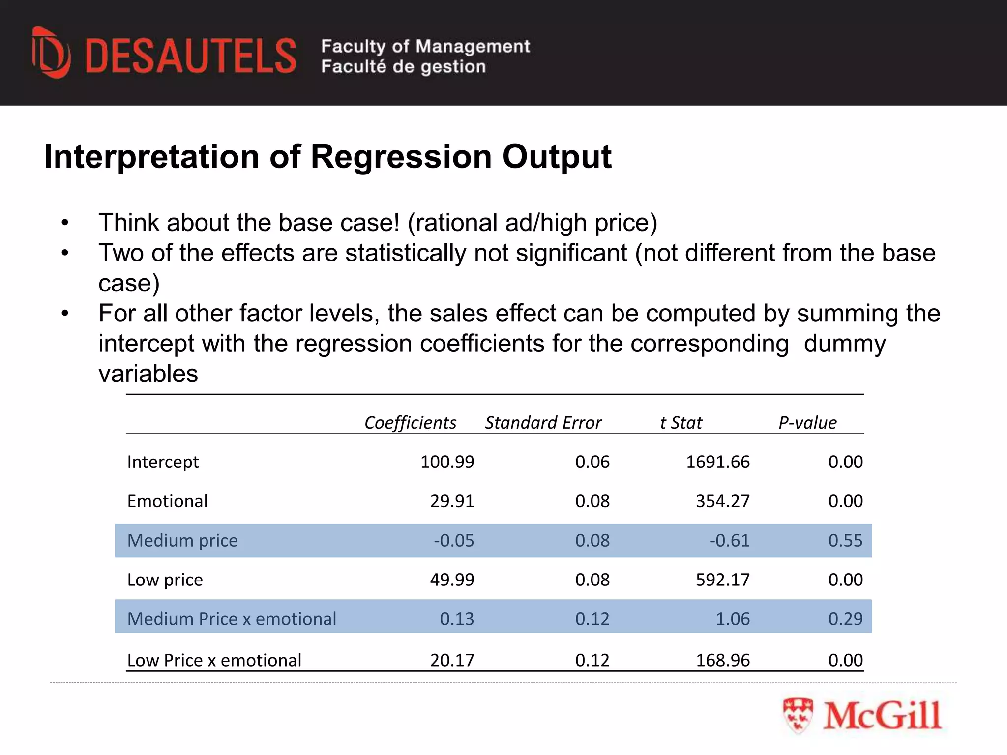
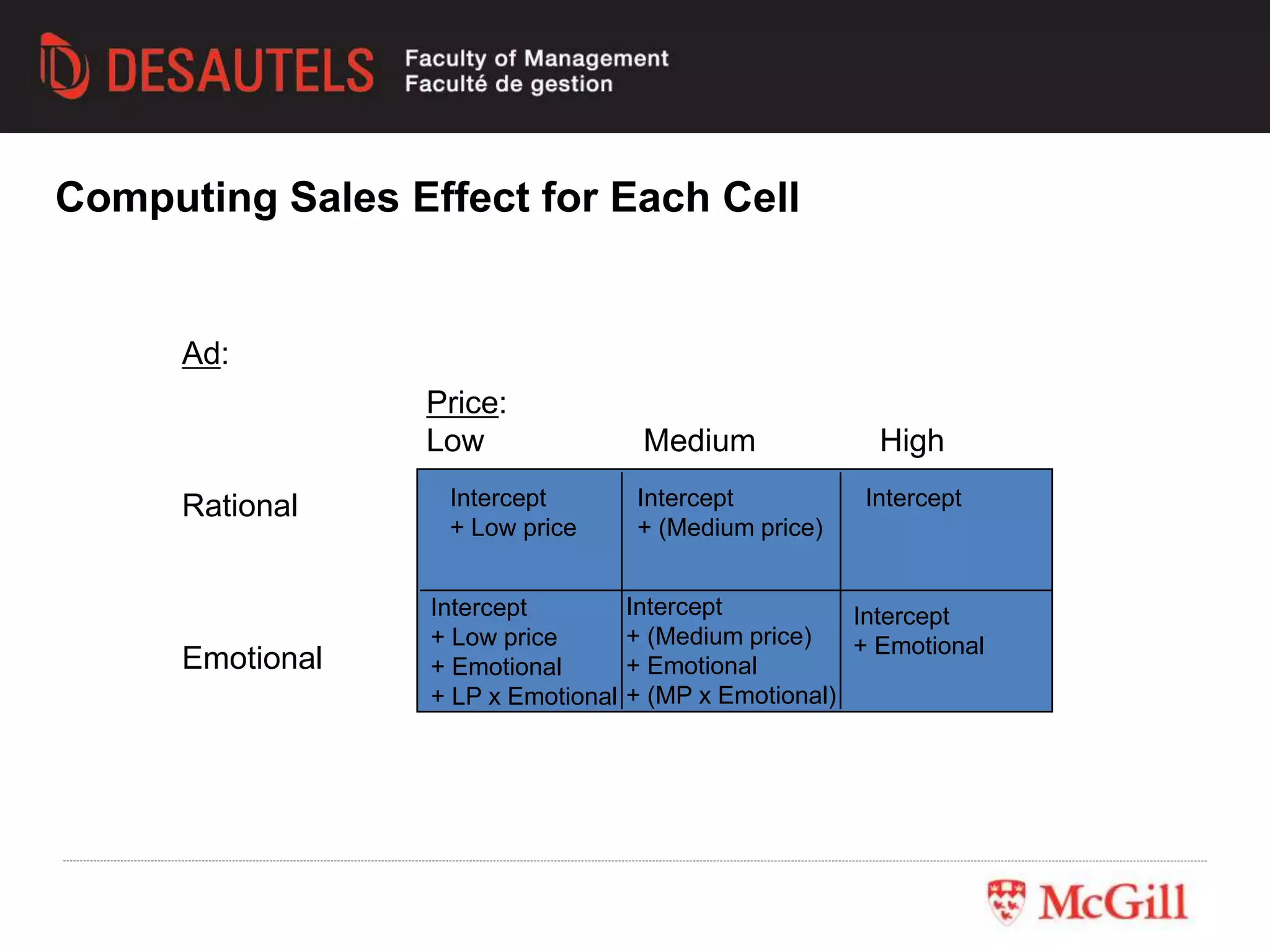
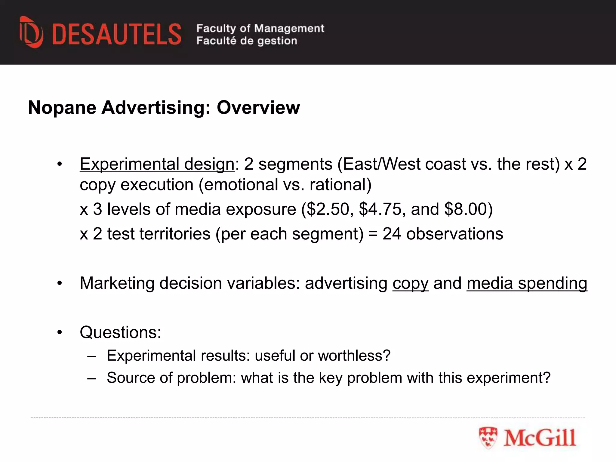
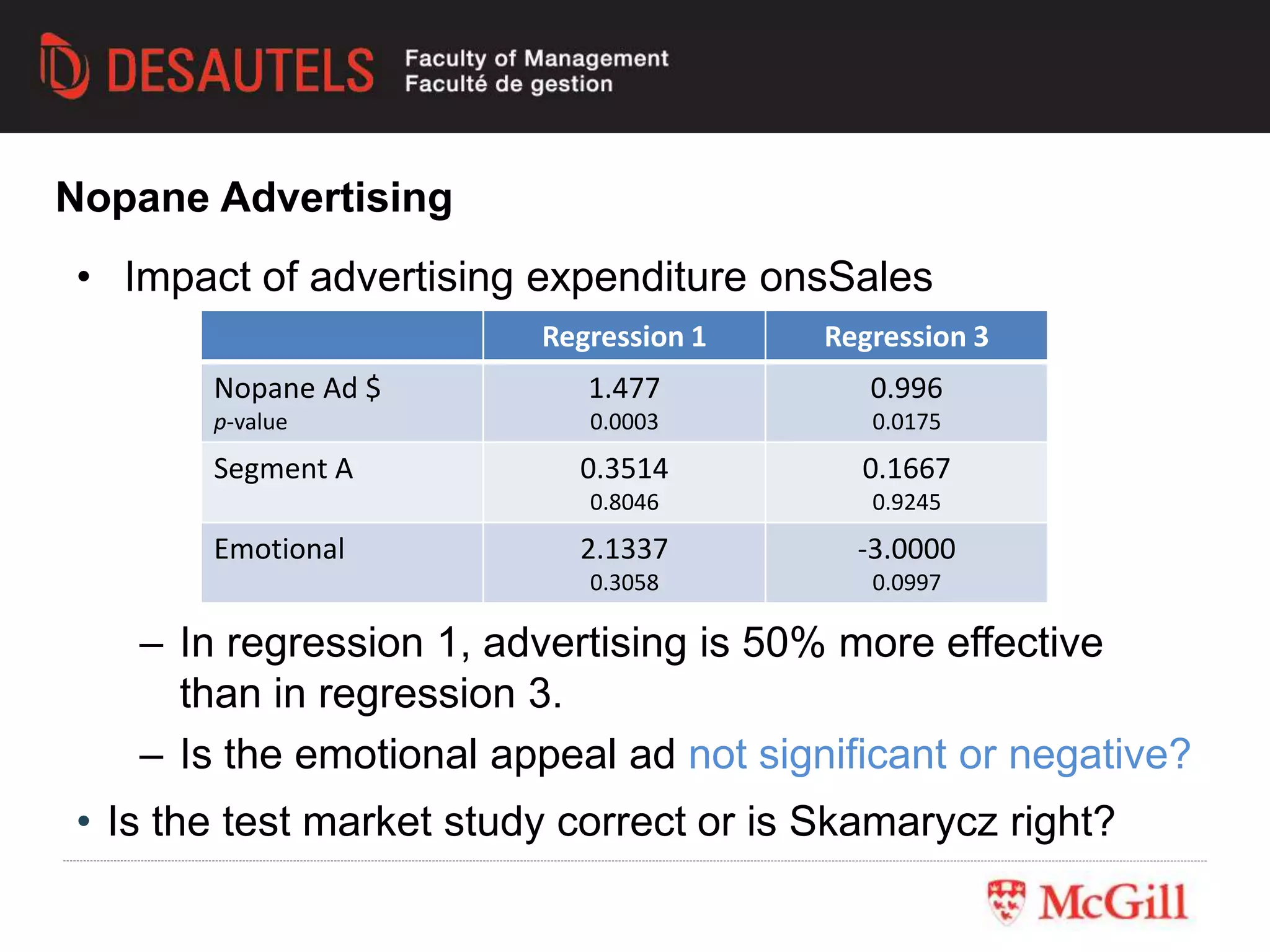
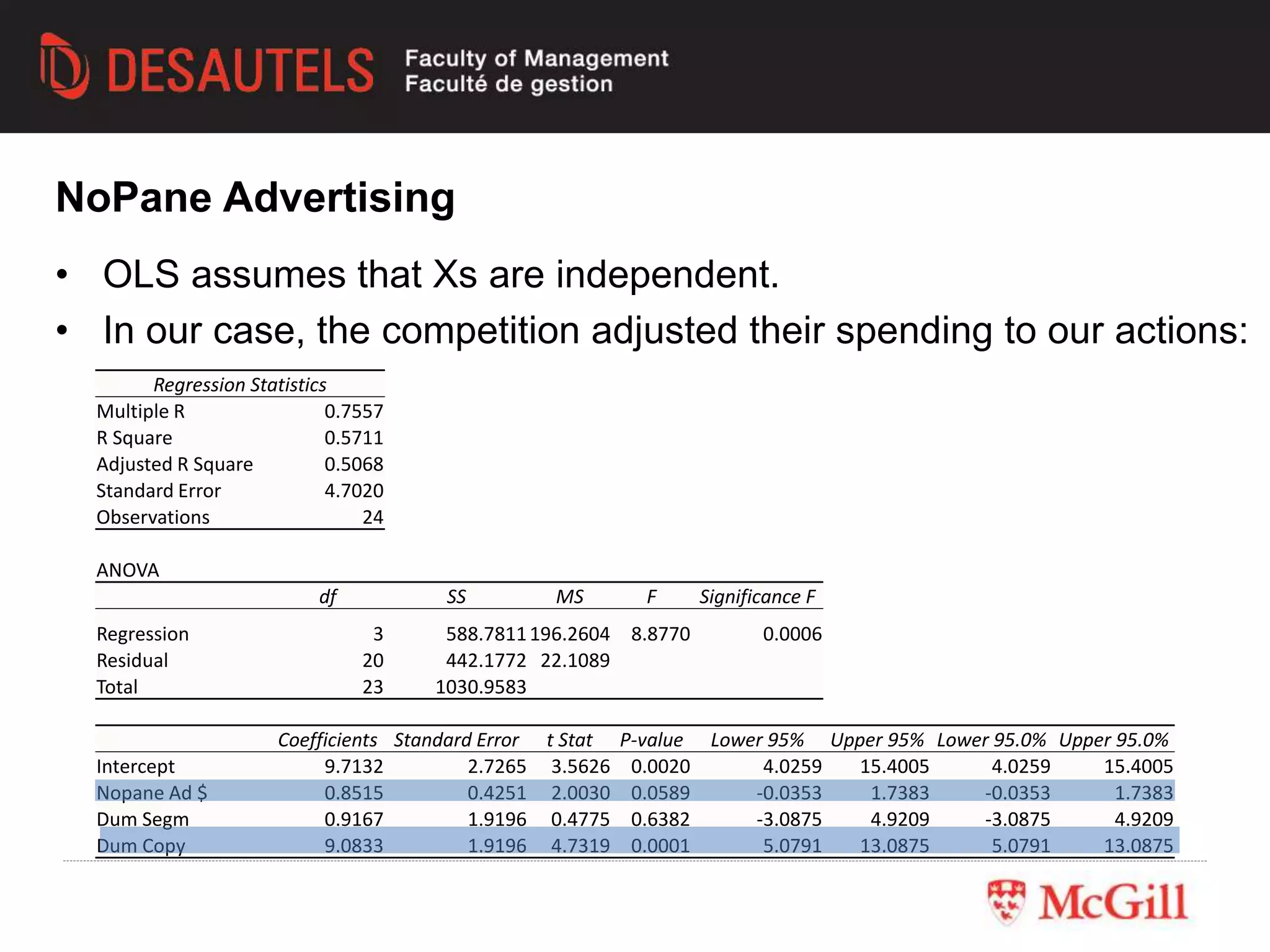
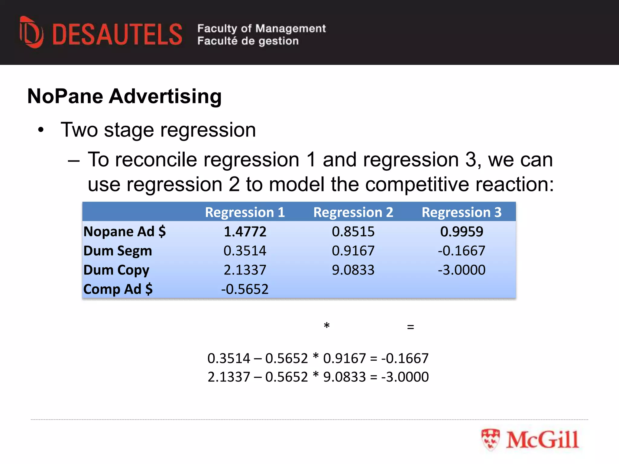
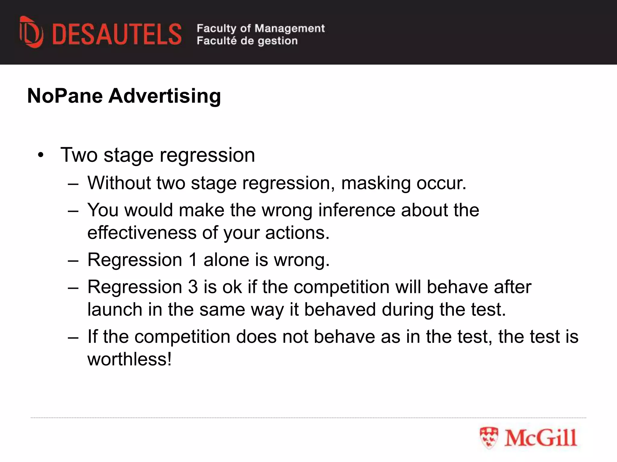
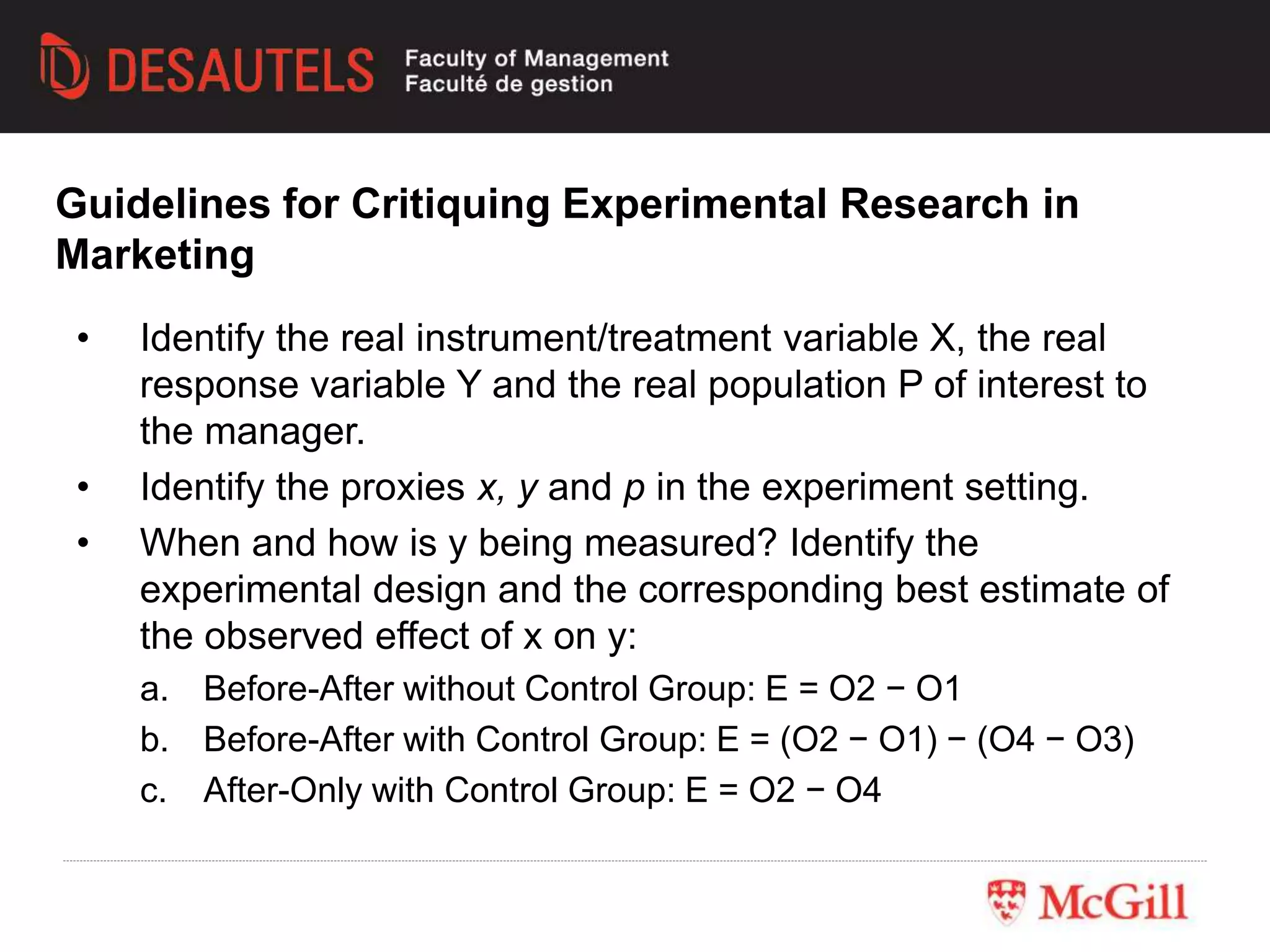
1. Marketing Research
MRKT 451
Experimentation II
February 7, 2010

2. • Within Subjects versus Between Subjects
• Field versus Lab Experiments
• ANOVA
• Regression
• Case: NoPane Advertising Strategy
• Guidelines for Critiquing Experimental Research
Class Outline

3. • Between-subjects design
– Each subject receives only one treatment.
– Comparisons are made between groups of different
subjects.
• Within-subjects design
– Subject receives more than one treatment.
– Comparisons are made across multiple measures on the
same subject.
Two types of experiments

4. • Within subjects designs are advantageous because you
get greater statistical power due to “internal matching”
(you are your own control).
• However, in some cases, due to contamination, time
constraints, between subjects designs must be used.
• This is not an obvious issue.
Within or Between Subjects?

5. (in-market) (paper/pencil)
High
External
Validity
High
Internal
Validity
Field Lab
Scientific
Control
Real world
Environment
Trade-offs: Field vs. Lab Experiments

6. Laboratory Field
Validity High Internal
Low External
Low Internal
High External
Time & Cost Low High
Exposure to Competition Low High
Nature of the Manipulation Realistic in a
contrived setting
Difficult to duplicate in
a lab
Trade-offs: Field vs. Lab Experiments

7. Analysis of Variance

8. • ”In our test mailing, did urban customers spend more
than rural customers?“
ANOVA: Comparison of Means

9. • Most of the time, we want to draw conclusions from our
sample about the population at large
– Know that in the test mailing urban customers spent more
than rural customers, $35.10 vs. $31.34
– Can we conclude from this that we can reliably expect that
this difference exists in our customer base at large? (Or is
this a “fluke” of our test mailing?)
– Is the average spending of rural customers statistically
significantly different from the average spending of urban
customers?
• Statistical inference allows us to make conclusions about
the population at large
Statistical Inference: Comparison of Means

10. • Statistical inference means deciding which of two
hypotheses to accept as likely to be true
In our example AvgExpurban – AvgExprural = $3.76
Question: Is this close to or far from 0?
Hypothesis 0
Average expenditures of urban
and rural customers are the same
Hypothesis 1
Average expenditures of urban
and rural customers are different
If true, we
expect…
If true, we
expect…
Statistical Inference

11. • Statistics enables us to conclude whether a value is “close to” or “far
from” zero
• Technically, a “statistic” is a number derived from a formula based
on data
– A mean is a statistic: the sum of the variable values divided by the
number of observations
– A variance is a statistic
• Statistical theory
– For example, we do not need to know the distribution of the
expenditures of the customers in the urban area
– But, if we take 10 sets of samples, and calculated the mean of each
sample, we do know how those means would be distributed
Statistical Inference

12. Statistically Meaningful Difference ~ f(variance)
• Generate data (sample size of 50) by randomly drawing from a normal distribution
N(33.22,52); Assign 25 samples for each group
• Group 1) Mean: 33.61
27.90 25.00 41.13 34.68 27.28
38.60 26.73 32.61 36.92 29.02
31.47 33.37 42.98 35.52 31.22
32.09 31.82 39.75 31.80 29.26
34.42 32.75 37.19 38.02 38.66
• Group 2) Mean: 31.92
36.46 36.38 42.74 27.42 31.48
24.74 37.82 33.33 31.72 24.61
34.14 31.92 26.45 27.43 29.41
31.97 24.98 32.31 36.30 31.34
29.73 34.74 38.73 30.99 30.89
• With std of 5,
difference of 1.69 can
be made by chance

13. Statistically Meaningful Difference ~ f(variance)
• Generate data (sample size of 50) by randomly drawing from a normal distribution
N(33.22,12); Assign 25 samples for each group
• Group 1) Mean: 33.33
31.78 32.24 33.83 33.11 33.98
33.89 33.60 33.99 34.74 33.80
33.65 33.18 31.98 32.72 33.55
32.11 33.69 33.54 33.32 33.52
33.24 33.20 33.21 34.15 33.13
• Group 2) Mean: 33.30
30.58 32.73 33.42 34.18 34.60
32.28 33.98 33.46 33.01 33.24
33.19 33.36 33.46 32.55 32.17
34.19 33.00 34.63 32.30 32.63
34.64 34.63 32.19 33.43 34.56
• With std of 1,
difference of 0.03 can
be made by chance

14. • 2 Population Means
– Two independent, separate target populations
• e.g., compare men vs. women on a rating scale
• e.g., compare users vs. nonusers on #oz purchased
– Draw random samples of sizes “n1” and “n2”
– Collect data:
• X11, X12, X13, ..., X1n
• X21, X22, X23, ..., X2m
– H0:
– Ha:
21  
21  
Hypothesis Testing: Comparison of means (2 groups)

15. • Compare 3 or more population means?
• F-test (ANOVA) extension of t-test to 3+ groups
• e.g., Three pricing strategies:
– Low
– Medium
– High
Analysis of Variance (ANOVA)

16. • Variance Between vs. Variance Within
price: high mdm low
sales,
p(buy),F= Var Betw Grps
-------------------
Var W/in Grps
F-test Intuitively

17. Group: I IIIII
Grand Mean
Yij
ijiijY  Model:
ANOVA: Model

18. SStotal = SSbetween groups + SSwithin groups
a n _
SStotal = ( yij - y..) 2
i=1 j=1
 
a n _ _
SSbetw = ( yi. - y..) 2
i=1 j=1
 
a n _
SSw/in = ( yij - yi.) 2
i=1 j=1
 
ANOVA: Computation

19. • MSbetween = SSbetween / (a - 1)
• MSwithin = SSwithin / (a * (n - 1))
• F = MSbetween / MSwithin
• F has (a - 1) and (a * (n - 1)) degrees of freedom
ANOVA: F-test

20. • Manipulate more than 1 factor:
– Random sample, randomly assign to 1 condition
– Combinations of 2 or more experimental factors
• Beard x UPS Logo
• Ad x Price
ANOVA: Logical Extension

21. • Brand Equity & Price Sensitivity
– 2x2: UPS/not branded x bearded/not bearded
– 2x3: 2 ad themes x 3 price strategies:
Price:
Low Mdm High
Ad:
Standard
Luxury
Multi-factor ANOVA: Example

22. • Is one ad more effective than another?
• Is one pricing level more effective than the others?
• Do the ads and prices “interact”?; is there any particular
combination of the ads and prices that is especially
effective? (Or detrimental?)
ANOVA Hypotheses

23. Regression

24. • Effect of Ad?
• Effect of Price?
• Effect of Ad x Price?
Model: ijkijjiijkY   )(
Experiment: Model

25. • 2 types of ad (rational vs. emotional) and 3 price levels (low, medium, or
high)
• 15 observations per each treatment
• Total number of observation = 2 x 3 x 15 = 90
Collected Data After Experiments
ID Group Ad type Price level Sales
1 1 Emotional High 129.92
2 1 Emotional High 131.45
.. .. .. .. ..
16 2 Emotional Medium 130.89
17 2 Emotional Medium 130.97
.. .. .. .. ..
89 6 Rational Low 151.12
90 6 Rational Low 151.32

26. • To obtain the size/existence of effects, we need to
understand how the various factor levels affect the
dependent variable (e.g. sales)
• A regression could be useful, but a regression is usually
for numerical variables and not for “categorical” variables
• We need to convert the categorical variables into
numerical variables. This is achieved by “dummy
variable coding”
• A dummy variable for interaction term can be made by
multiplying relevant level of factors
Data processing

27. • We need one dummy variable for every factor level in
the experiment
• For a certain treatment, the dummy variable for a certain
factor level takes value 1 if that treatment contains the
factor level and takes value 0 otherwise.
Dummy Variable Coding
In our example, the total number of dummy variables needed for
main effects is 2 (ad) + 3 (price) = 5
For each factor, replace the column containing the factor level
with columns containing the values of the corresponding dummy
variables.

28. • 2 dummy variables for ad types
• 3 dummy variables for price levels
• Interaction terms are not considered yet
Dataset After Initial Dummy Variable Coding
ID Group d_em_ad d_ra_ad d_hp d_mp d_lp Sales
1 1 1 0 1 0 0 129.92
2 1 1 0 1 0 0 131.45
.. .. .. .. .. .. .. ..
16 2 1 0 0 1 0 130.89
17 2 1 0 0 1 0 130.97
.. .. .. .. .. .. .. ..
89 6 0 1 0 0 1 151.12
90 6 0 1 0 0 1 151.32

29. Dummy Variable Regression
• We need to run a regression with sales as the y variable
and the dummies as the x variables.
• Problem: Within any one factor, the dummies are
perfectly correlated
– The value of one dummy can be inferred from the rest
– Perfect multicollinearity
– Creates problems for most regression software

30. Solution
• For each factor
– Pick any one factor level. We will call this the “base case”
level for the factor
– Eliminate the dummy corresponding to the base case
• Run a regression using the remaining variables. Tabulate the
coefficients.
Total number of factor
levels in the experiment
Total number of factors
in the experiment
Excluding the intercept term, the total number of variables
in this regression will be:

31. Taking out Dummy Variables for the Base Case
• Suppose, we choose the base case factor level of each
attribute as follows
– Ad type: Rational (base case)
– Price level: High price (base case)
• The x variables (for main effects) in the regression will
be: d_em_ad, d_lp, and d_mp (3 variables)
• Now, we can create dummy variables for interaction
terms by multiplying the remaining levels of each factor

32. • 1 dummy variable for ad types (main effects)
• 2 dummy variables for price levels (main effects)
• 2 dummy variables for interaction terms
Final Dataset with Dummy Variables for Interaction
Terms
ID Group d_em_ad d_mp d_lp d_int_e
m_mp
d_int_e
m_lp
Sales
1 1 1 0 0 0 0 129.92
2 1 1 0 0 0 0 131.45
.. .. .. .. .. ..
16 2 1 1 0 1 0 130.89
17 2 1 1 0 1 0 130.97
.. .. .. .. .. ..
89 6 0 0 1 0 0 151.12
90 6 0 0 1 0 0 151.32

33. Interpretation of Regression Output
• After running a regression analysis, we obtain the
following results.
• How should we interpret the results?
Coefficients Standard Error t Stat P-value
Intercept 100.99 0.06 1691.66 0.00
Emotional 29.91 0.08 354.27 0.00
Medium price -0.05 0.08 -0.61 0.55
Low price 49.99 0.08 592.17 0.00
Medium Price x emotional 0.13 0.12 1.06 0.29
Low Price x emotional 20.17 0.12 168.96 0.00

34. • Interpretations
– F-Statistics: Omnibus test that all coefficients are 0.
• Numerator degrees of freedom is the number of Xs (k) in the
model.
• Denominator is n-k-1.
– t-Statistics: Test for individual coefficients = 0.
– p-value: The probability of observing the data we did
given the null hypothesis is true.
Interpretations: Linear Regression

35. Interpretation of Regression Output
• Think about the base case! (rational ad/high price)
• Two of the effects are statistically not significant (not different from the base
case)
• For all other factor levels, the sales effect can be computed by summing the
intercept with the regression coefficients for the corresponding dummy
variables
Coefficients Standard Error t Stat P-value
Intercept 100.99 0.06 1691.66 0.00
Emotional 29.91 0.08 354.27 0.00
Medium price -0.05 0.08 -0.61 0.55
Low price 49.99 0.08 592.17 0.00
Medium Price x emotional 0.13 0.12 1.06 0.29
Low Price x emotional 20.17 0.12 168.96 0.00

36. Price:
Low Medium High
Ad:
Rational
Emotional
Intercept
+ Low price
Intercept
+ Low price
+ Emotional
+ LP x Emotional
Intercept
+ (Medium price)
Intercept
Intercept
+ (Medium price)
+ Emotional
+ (MP x Emotional)
Intercept
+ Emotional
Computing Sales Effect for Each Cell

37. Nopane Advertising Strategy

38. • Experimental design: 2 segments (East/West coast vs. the rest) x 2
copy execution (emotional vs. rational)
x 3 levels of media exposure ($2.50, $4.75, and $8.00)
x 2 test territories (per each segment) = 24 observations
• Marketing decision variables: advertising copy and media spending
• Questions:
– Experimental results: useful or worthless?
– Source of problem: what is the key problem with this experiment?
Nopane Advertising: Overview

39. • Impact of advertising expenditure onsSales
– In regression 1, advertising is 50% more effective
than in regression 3.
– Is the emotional appeal ad not significant or negative?
• Is the test market study correct or is Skamarycz right?
Regression 1 Regression 3
Nopane Ad $
p-value
1.477
0.0003
0.996
0.0175
Segment A 0.3514
0.8046
0.1667
0.9245
Emotional 2.1337
0.3058
-3.0000
0.0997
Nopane Advertising

40. • OLS assumes that Xs are independent.
• In our case, the competition adjusted their spending to our actions:
Regression Statistics
Multiple R 0.7557
R Square 0.5711
Adjusted R Square 0.5068
Standard Error 4.7020
Observations 24
ANOVA
df SS MS F Significance F
Regression 3 588.7811196.2604 8.8770 0.0006
Residual 20 442.1772 22.1089
Total 23 1030.9583
Coefficients Standard Error t Stat P-value Lower 95% Upper 95% Lower 95.0% Upper 95.0%
Intercept 9.7132 2.7265 3.5626 0.0020 4.0259 15.4005 4.0259 15.4005
Nopane Ad $ 0.8515 0.4251 2.0030 0.0589 -0.0353 1.7383 -0.0353 1.7383
Dum Segm 0.9167 1.9196 0.4775 0.6382 -3.0875 4.9209 -3.0875 4.9209
Dum Copy 9.0833 1.9196 4.7319 0.0001 5.0791 13.0875 5.0791 13.0875
NoPane Advertising

41. • Two stage regression
– To reconcile regression 1 and regression 3, we can
use regression 2 to model the competitive reaction:
Regression 1 Regression 2 Regression 3
Nopane Ad $ 1.4772 0.8515 0.9959
Dum Segm 0.3514 0.9167 -0.1667
Dum Copy 2.1337 9.0833 -3.0000
Comp Ad $ -0.5652
0.3514 – 0.5652 * 0.9167 = -0.1667
2.1337 – 0.5652 * 9.0833 = -3.0000
1.4772
-0.5652
0.8515
* =
0.9959
NoPane Advertising

42. • Two stage regression
– Without two stage regression, masking occur.
– You would make the wrong inference about the
effectiveness of your actions.
– Regression 1 alone is wrong.
– Regression 3 is ok if the competition will behave after
launch in the same way it behaved during the test.
– If the competition does not behave as in the test, the test is
worthless!
NoPane Advertising

43. Guidelines for Critiquing
Experimental Research

44. • Identify the real instrument/treatment variable X, the real
response variable Y and the real population P of interest to
the manager.
• Identify the proxies x, y and p in the experiment setting.
• When and how is y being measured? Identify the
experimental design and the corresponding best estimate of
the observed effect of x on y:
a. Before-After without Control Group: E = O2 − O1
b. Before-After with Control Group: E = (O2 − O1) − (O4 − O3)
c. After-Only with Control Group: E = O2 − O4
Guidelines for Critiquing Experimental Research in
Marketing

45. • Look for problems in internal validity.
– Are there alternative explanations to the change E other
than the treatment variable? If there are, the statement
that x causes y is falsifiable and the experiment is flawed.
• Look for problems in external validity. That is, is there a
problem with the proxies?
Guidelines for Critiquing Experimental Research in
Marketing

46. • Read Chap. 11 of Text
• Read “The Science of Asking Questions”
• Individual assignment #1 (experimentation) will be
handed out on Wednesday
For next class…