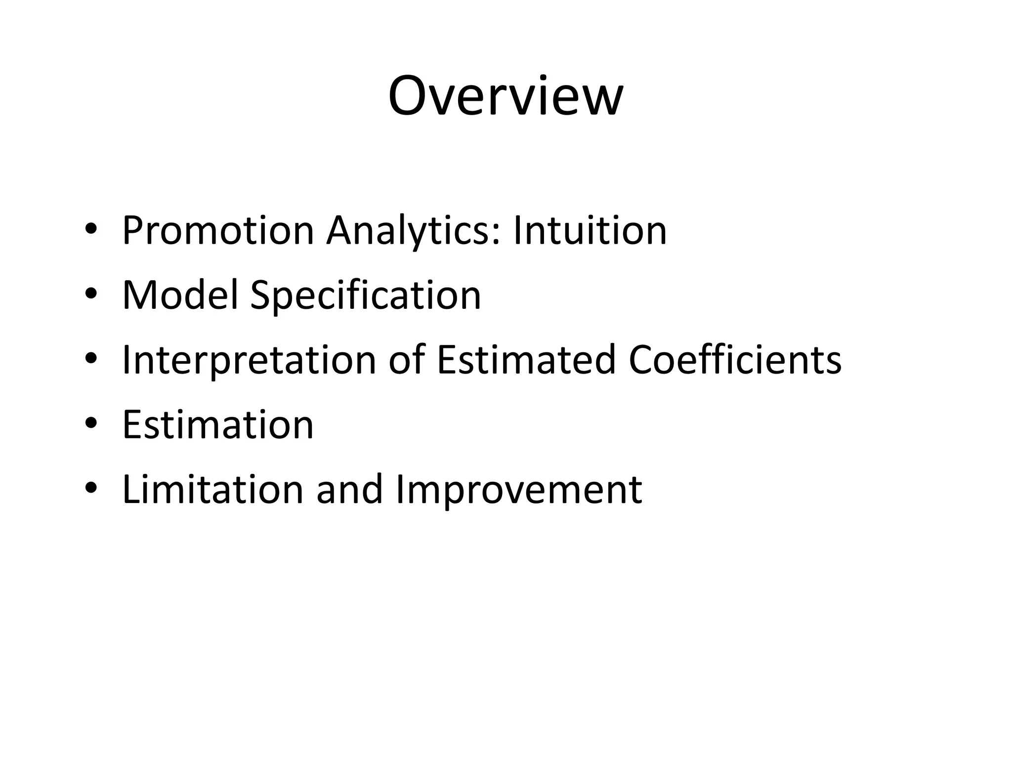
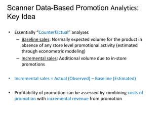
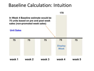
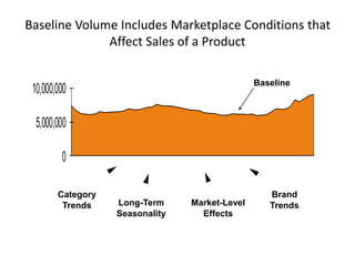
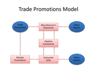
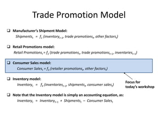
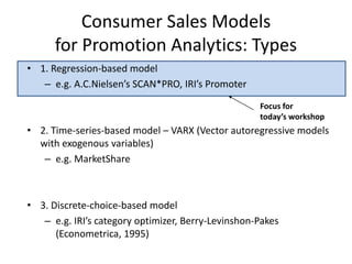
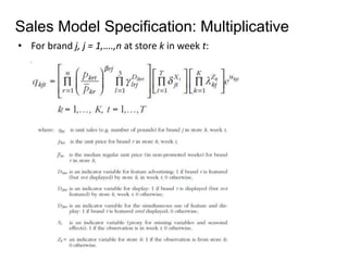
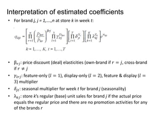
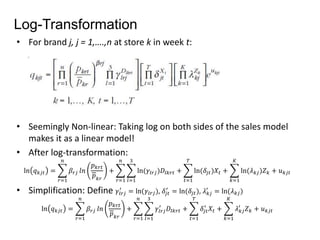
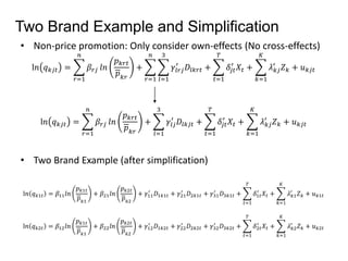
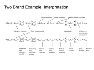
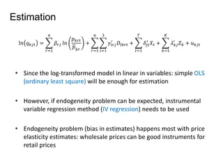
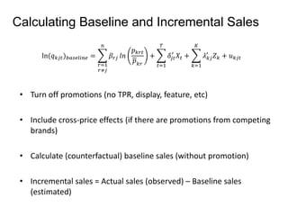
This document provides an overview of promotion analytics using scanner data. It discusses estimating baseline and incremental sales from promotions through econometric modeling. Key aspects covered include model specification, interpretation of coefficients, and limitations. The modeling approach involves log-transforming a multiplicative sales model to make it linear and estimating it using ordinary least squares regression. Baseline sales are estimated by turning off promotions, and incremental sales are calculated as the difference between actual and baseline sales.

1. Overview
• Promotion Analytics: Intuition
• Model Specification
• Interpretation of Estimated Coefficients
• Estimation
• Limitation and Improvement

2. Scanner Data-Based Promotion Analytics:
Key Idea
• Essentially “Counterfactual” analyses
– Baseline sales: Normally expected volume for the product in
absence of any store level promotional activity (estimated
through econometric modeling)
– Incremental sales: Additional volume due to in-store
promotions
• Incremental sales = Actual (Observed) – Baseline (Estimated)
• Profitability of promotion can be assessed by combining costs of
promotion with incremental revenue from promotion

3. The Analytic Path
Most issues can be addressed by drilling down this path
Issue
Base Volume Incremental Volume
Distribution Velocity
% ACV
(Breadth)
# of Items
(Depth)
Base Price
Competitive
Activity
Other Factors
Promotion
Support
(Quantity)
Promotion
Effectiveness
(Quality)
Level of
Support
Promo Mix
Promo Price
Price Discount
Competitive Activity

4. Baseline Calculation: Intuition
170
In Week 4 Baseline estimate would be
75 units based on pre and post week
sales (non-promoted week sales)
Unit Sales
75
75 75 75 75
Display
Week
week 1 week 2 week 3 week 4 week 5

5. Baseline Volume Includes Marketplace Conditions that
Affect Sales of a Product
10,000,000
5,000,000
0
Category
Trends Long-Term
Seasonality
Market-Level
Effects
Baseline
Brand
Trends

6. Trade Promotions Model
Pipeline
Inventories
Trade
Promotions
Manufacturer’s
Shipments
Other
Factors
Consumer
Sales
Retailer
Promotions
Other
Factors

7. Trade Promotion Model
 Manufacturer’s Shipment Model:
Shipmentst = f1 (inventoryt–1, trade promotionst, other factorst)
 Retail Promotions model:
Retail Promotionst = f2 (trade promotionst, trade promotionst–1, inventoriest–1)
 Consumer Sales model:
Consumer Salest = f3 (retailer promotionst, other factorst)
 Inventory model:
Inventoryt = f4 (inventoriest–1, shipmentst, consumer salest)
 Note that the Inventory model is simply an accounting equation, as:
Inventoryt = Inventoryt–1 + Shipmentst – Consumer Salest
Focus for
today’s workshop

8. Consumer Sales Models
for Promotion Analytics: Types
Focus for
today’s workshop
• 1. Regression-based model
– e.g. A.C.Nielsen’s SCAN*PRO, IRI’s Promoter
• 2. Time-series-based model – VARX (Vector autoregressive models
with exogenous variables)
– e.g. MarketShare
• 3. Discrete-choice-based model
– e.g. IRI’s category optimizer, Berry-Levinshon-Pakes
(Econometrica, 1995)

9. Sales Model Specification: Multiplicative
• For brand j, j = 1,….,n at store k in week t:

10. Interpretation of estimated coefficients
• For brand j, j = 1,….,n at store k in week t:
• β푟푗 : price discount (deal) elasticities (own-brand if 푟 = 푗, cross-brand
if 푟 ≠ 푗
• 훾푙푟푗: feature-only (푙 = 1), display-only (푙 = 2), feature & display (푙 =
3) multiplier
• 훿푗푡: seasonal multiplier for week t for brand j (seasonality)
• λ푘푗 : store k’s regular (base) unit sales for brand j if the actual price
equals the regular price and there are no promotion activities for any
of the brands r

11. Log-Transformation
• For brand j, j = 1,….,n at store k in week t:
• Seemingly Non-linear: Taking log on both sides of the sales model
makes it as a linear model!
• After log-transformation:
l푛 푞푘푗푡 =
푛
푟=1
훽푟푗 푙푛
푝푘푟푡
푝푘푟
+
푛
푟=1
3
푙=1
ln(훾푙푟푗 )퐷푙푘푟푡 +
푇
푡=1
ln(훿푗푡 )푋푡 +
퐾
푘=1
ln(휆푘푗 )푍푘 + 푢푘푗푡
• Simplification: Define 훾푙푟푗
′ = ln(훾푙푟푗 ), 훿푗푡
′ = ln(훿푗푡 ), 휆푘푗
′ = ln(휆푘푗 )
l푛 푞푘푗푡 =
푛
푟=1
훽푟푗 푙푛
푝푘푟푡
푝푘푟
+
푛
푟=1
3
푙=1
′ 퐷푙푘푟푡 +
훾푙푟푗
푇
푡=1
′ 푋푡 +
훿푗푡
퐾
푘=1
′ 푍푘 + 푢푘푗푡
휆푘푗

12. Two Brand Example and Simplification
• Non-price promotion: Only consider own-effects (No cross-effects)
l푛 푞푘푗푡 =
푛
푟=1
훽푟푗 푙푛
푝푘푟푡
푝푘푟
+
푛
푟=1
3
푙=1
′ 퐷푙푘푟푡 +
훾푙푟푗
푇
푡=1
′ 푋푡 +
훿푗푡
퐾
푘=1
′ 푍푘 + 푢푘푗푡
휆푘푗
l푛 푞푘푗푡 =
푛
푟=1
훽푟푗 푙푛
푝푘푟푡
푝푘푟
+
3
푙=1
′ 퐷푙푘푗푡 +
훾푙푗
푇
푡=1
′ 푋푡 +
훿푗푡
퐾
푘=1
′ 푍푘 + 푢푘푗푡
휆푘푗
• Two Brand Example (after simplification)
l푛 푞푘1푡 = 훽11푙푛
푝푘1푡
푝푘1
+ 훽21푙푛
푝푘2푡
푝푘2
′ 퐷1푘1푡 + 훾21
+ 훾11
′ 퐷2푘1푡 + 훾31
′ 퐷3푘1푡 +
푇
푡=1
′ 푋푡 +
훿1푡
퐾
푘=1
′ 푍푘 + 푢푘1푡
휆푘1
l푛 푞푘2푡 = 훽12푙푛
푝푘1푡
푝푘1
+ 훽22푙푛
푝푘2푡
푝푘2
′ 퐷1푘2푡 + 훾22
+ 훾12
′ 퐷2푘2푡 + 훾32
′ 퐷3푘2푡 +
푇
푡=1
′ 푋푡 +
훿2푡
퐾
푘=1
′ 푍푘 + 푢푘2푡
휆푘2

13. Two Brand Example: Interpretation
l푛 푞푘1푡 = 훽11푙푛
푝푘1푡
푝푘1
+ 훽21푙푛
푝푘2푡
푝푘2
′ 퐷1푘1푡 + 훾21
+ 훾11
′ 퐷2푘1푡 + 훾31
′ 퐷3푘1푡 +
푇
푡=1
′ 푋푡 +
훿1푡
퐾
푘=1
′ 푍푘 + 푢푘1푡
휆푘1
Own price elasticity Cross price elasticity
l푛 푞푘2푡 = 훽12푙푛
푝푘1푡
푝푘1
+ 훽22푙푛
푝푘2푡
푝푘2
′ 퐷1푘2푡 + 훾22
+ 훾12
′ 퐷2푘2푡 + 훾32
′ 퐷3푘2푡 +
푇
푡=1
′ 푋푡 +
훿2푡
퐾
푘=1
′ 푍푘 + 푢푘2푡
휆푘2
Week
dummy
Store
dummy
Residual
error
Feature
only
indicator
Display
only
indicator
Feature-display
indicator
Temporary
price
reduction:
brand 1
Temporary
price
reduction:
brand 2
Feature multiplier Display multiplier Feature-display multiplier
Seasonality Difference in
baseline sales
across stores

14. Estimation
l푛 푞푘푗푡 =
푛
푟=1
훽푟푗 푙푛
푝푘푟푡
푝푘푟
+
푛
푟=1
3
푙=1
′ 퐷푙푘푟푡 +
훾푙푟푗
푇
푡=1
′ 푋푡 +
훿푗푡
퐾
푘=1
′ 푍푘 + 푢푘푗푡
휆푘푗
• Since the log-transformed model in linear in variables: simple OLS
(ordinary least square) will be enough for estimation
• However, if endogeneity problem can be expected, instrumental
variable regression method (IV regression) needs to be used
• Endogeneity problem (bias in estimates) happens most with price
elasticity estimates: wholesale prices can be good instruments for
retail prices

15. Calculating Baseline and Incremental Sales
ln(푞푘푗푡)푏푎푠푒푙푖푛푒 =
푛
푟=1
푟≠푗
훽푟푗 푙푛
푝푘푟푡
푝푘푟
+
푇
푡=1
′ 푋푡 +
훿푗푡
퐾
푘=1
′ 푍푘 + 푢푘푗푡
휆푘푗
• Turn off promotions (no TPR, display, feature, etc)
• Include cross-price effects (if there are promotions from competing
brands)
• Calculate (counterfactual) baseline sales (without promotion)
• Incremental sales = Actual sales (observed) – Baseline sales
(estimated)

16. Limitation
• Curse of dimensionality: Not very scalable in the case of categories with
many SKUs -> J SKU’s: J x J parameters for each marketing mix
• Homogeneity in response parameters: More flexible models allow
heterogeneity in responses across chains/stores
• No consideration of dynamics: lags and leads of prices can be included for
dynamics
• Log-linearity assumption on deal effect: More flexible (semi-parametric)
models can be developed
• Potential endogeneity (bias in estimated effects) if there are systematic
allocation of promotion based on market/store conditions: instrumental
variable regression can be considered

17. Evolutionary Model Building: Example