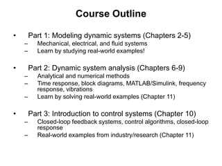
This document provides an introduction and overview of a course on dynamic systems and control (DSC). The course aims to teach students how to model, analyze, and design physical systems like mechanical, electrical, and fluid systems. It will cover modeling dynamic systems using differential equations, analyzing system response using analytical and numerical methods, and introducing feedback control systems. Students will learn through both theoretical discussions and real-world examples from industry. The course outline indicates it will cover topics like modeling different physical systems, dynamic response analysis in time and frequency domains, and feedback control design.

1. Chapter 1: Introduction to Dynamic
Systems and Control (DSC)
• In engineering problems, there is a need to understand
and determine the dynamic response of a physical
system that may involve several components
• These efforts involve modeling, analysis, simulation, and
design of physical systems
– Building a prototype system and conducting experiments/tests is
not feasible and/or is too expensive for preliminary design
– Mathematical modeling and analysis of engineering systems
greatly aid the design process

2. DSC: Definitions
• System: A combination of components acting together to perform a
specified objective. The components or interacting elements have
cause-and-effect (or input/output) relationships. We will investigate
mechanical, electrical, fluid, and mixed systems.
• Dynamic system: The current output variables of a system depend
on the initial conditions (or stored energy) of the system and/or the
previous input variables. The dynamic variables of the system (e.g.,
displacement, velocity, voltage, pressure, etc) vary with time.
• Modeling: The process of applying the appropriate fundamental
physical laws in order to derive mathematical equations that
adequately describe the physics of the engineering system.
• Mathematical models: A mathematical description of a system’s
behavior, usually a set of differential equations for a dynamic system

3. DSC: Definitions (2)
• Simulation: The process of obtaining the system’s dynamic
response by numerically solving the governing modeling equations.
Simulation involves numerical integration of the model’s differential
equations and is performed by digital computers and simulation
software.
• System analysis: The use of analytical calculations or numerical
simulation tools to determine the system response in order to
assess its performance.

4. 1.2 Classification of Dynamic Systems
• Spatial characteristics
– Distributed (PDEs) vs. lumped parameters (ODEs)
• Time variable continuity
– “Analog” vs. “digital”
• Time dependence
– Time-varying vs. time-invariant parameters
• Superposition property
– Linear vs. nonlinear systems
Red bold-face: focus of DSC textbook

5. Spatial Characteristics
• Distributed system: infinite number of “internal”
variables; system is governed by PDE
– Example: continuous twist angle for shaft under
external torque
• Lumped system: finite number of “internal”
variables; system is governed by ODE
– Example: lump all inertia, stiffness, etc into single
elements; single twist angle of free end of shaft
under external torque
Red bold-face: focus of DSC textbook

6. Time Variable Continuity
Red bold-face: focus of DSC textbook
Continuous-time system (“analog”) Discrete-time system (“digital”)

7. Time Dependence
Red bold-face: focus of DSC textbook
• Time-varying system: system parameters change with
time
– Example: springs/shocks “wear out” over time
• Time-invariant system: constant system parameters
– Example: spring stiffness remains constant over time
– Therefore, identical inputs and initial conditions produce identical
dynamic responses every trial

8. Superposition (Linear vs. Nonlinear)
• Linear systems obey the superposition property :
1. If u1 is an input, and y1 = f(u1) is the corresponding
output, then ay1 = f(au1) , where a = any constant
2. If y1 = f(u1) and y2 = f(u2) , then y1 + y2 = f(u1+u2)
– Nonlinear systems do not obey these properties
– All physical systems are nonlinear. However, if we confine the
input/output variables to a restricted (nominal) range, then we
can replace a nonlinear system with a linear model.
– Linear dynamic systems are governed by linear differential
equations

9. Linear and Nonlinear ODEs
• Examples of linear ODEs:
• Examples of nonlinear ODEs:
u
x
x
x 2
9
4 

 


u
x
t
x
x 2
)
3
cos
9
(
4 


 


Linear time-invariant (LTI) ODE
Linear time varying ODE
u
x
x
x
x 2
9
4 

 


u
x
x
x 2
3
6 2


 



10. 1.3 Modeling Dynamic Systems
• Mathematical models are obtained by applying the
appropriate laws of physics to each element of a system
– Some system parameters (such as damping) may be unknown,
or these parameters are often determined through experiments
which lead to empirical relations
• Engineering judgment must be used to trade model
complexity with accuracy of the analysis
– Nonlinearities (such as gear backlash) are often ignored in
preliminary design studies in order to derive linear models
– Sometimes, low-order linear models can be solved analytically
– Furthermore, simulations (e.g., MATLAB/Simulink) are easier to
construct with low-order linear models and therefore system-
analysis time is reduced

11. Modeling Dynamic Systems (2)
• Engineers must remember that the results from a model
and/or simulation are only approximate and are valid
only to the extent of the assumptions used to derive the
model
• The model must be sufficiently sophisticated to
demonstrate the significant features of the dynamic
response without becoming too cumbersome for
available analysis tools
– Higher-order, complex nonlinear models typically require smaller
integration time steps to accurately solve the governing
differential equations, which increases computer run time
– Consequently, there is usually a trade-off between model
complexity and analysis time
– The validity of a mathematical model can often be verified by
comparing the model solution (i.e., simulation results) with
experimental results

12. High-Fidelity Modeling Examples
• Shuttle Vehicle Dynamics (SVD) was a computer
simulation for analyzing the separation dynamics
between the Space Shuttle and its solid rocket boosters
– SVD uses mathematical models for aerodynamic forces,
propulsion forces, spring and damper forces at interconnection
points, etc
• Shuttle Avionics Integration Lab (SAIL) at NASA Johnson
Space Center was used to simulate the dynamics of the
entire Space Shuttle mission profile
– SAIL was composed of “hardware in the loop” (such as sensors and
cockpit displays) mixed with mathematical models (such as
aerodynamic force models, gravity force models) and flight software
(such as guidance, navigation, and control functions)
– SAIL results compared very well with actual measured flight

13. Simulation Tools
• Simulink is a numerical simulation tool that is part of the
MATLAB software package developed by MathWorks
– Uses a graphical user interface (GUI) to develop a block diagram
representation of dynamic systems.
– Simulink is used by engineers in industry and academia.
– Constructing system models with Simulink is relatively easy and
therefore it is often used to build simple models during the
preliminary design stage.

14. Simulation Tools (2)
• Caterpillar developed and uses a computer simulation
tool called Dynasty to model and analyze integrated
hydraulic systems and hydraulic controls
– Dynasty models mechanical components (pistons, linkages,
springs), electrical components (servos, solenoids), and fluid
components (pressures in hoses, cylinders, accumulators).

15. Caterpillar’s Dynasty Software
Dynasty software lets Caterpillar engineers take new vehicles for test rides long
before physical prototypes are available. Taking sharp turns lets user see, for
example, whether or not there is sufficient room for wheel dynamics and how the
dump body shifts in turns.
(article in MachineDesign.com, November 6, 2003, by Paul Dvorak)
Dynasty lets users focus on performance modeling, not the underlying math
and physics. Users build schematic machines by dragging and dropping components
and connecting them together.
The software comes with more than 230
components such as engines, controls,
electronics, fluids, linkages, body
structures, and drivelines.
After building a model, the program
converts components and associated
design and performance data to symbolic
equations.

16. Simulation Tools (3)
• Boeing developed and uses a graphical simulation tool
called EASY5 which can model complete integrated
systems
– User can construct integrated systems from menu of sub-
systems (mechanical, electrical, or hydraulic)
From MCS Software webpage:
“Adams and MD Adams provide accurate and efficient multi-body dynamics and
motion analysis of 3D mechanical systems. The core package (Adams/View,
Adams/Solver, and Adams/PostProcessor) allows you to import geometry from
most major CAD systems or to build a solid model of the mechanical system from
scratch. Adams models can be integrated with EASY5 controls models directly,
or via co-simulation for full multidiscipline analysis.”

17. 1.4 Objectives
• Introduce students to the mathematical modeling of
physical systems
– Mechanical, electrical, fluid, and thermal systems
– Show “real-world” examples from ASME articles, industry
• Introduce students to analytical and numerical
methods for obtaining a system’s dynamic response to
various initial conditions and input functions
– Analytical: solving ODEs “by hand”
– Numerical: MATLAB and Simulink
• Analyze and design feedback control systems in order
to achieve a desirable system response

18. Course Outline
• Part 1: Modeling dynamic systems (Chapters 2-5)
– Mechanical, electrical, and fluid systems
– Learn by studying real-world examples!
• Part 2: Dynamic system analysis (Chapters 6-9)
– Analytical and numerical methods
– Time response, block diagrams, MATLAB/Simulink, frequency
response, vibrations
– Learn by solving real-world examples (Chapter 11)
• Part 3: Introduction to control systems (Chapter 10)
– Closed-loop feedback systems, control algorithms, closed-loop
response
– Real-world examples from industry/research (Chapter 11)