Basic Integral Calculus

1
INTEGRATION BASIC
A SHORT NOTES
Arun Umrao
https://sites.google.com/view/arunumrao
DRAFT COPY - GPL LICENSING

2 Integration
Contents
1 Integration 3
1.1 Continuous Sampling . . . . . . . . . . . . . . . . . . . . . . . 5
1.1.1 First Order Adder . . . . . . . . . . . . . . . . . . . . 5
1.1.2 Second Order Adder . . . . . . . . . . . . . . . . . . . 6
1.2 Antiderivative . . . . . . . . . . . . . . . . . . . . . . . . . . . 11
1.2.1 First Principle Method . . . . . . . . . . . . . . . . . . 12
1.2.2 Lower & Upper Bound . . . . . . . . . . . . . . . . . . 20
1.2.3 Integral As Summation . . . . . . . . . . . . . . . . . . 27
1.3 Direct Integration . . . . . . . . . . . . . . . . . . . . . . . . . 35
1.3.1 Error/Residual . . . . . . . . . . . . . . . . . . . . . . 56
1.3.2 Inverse Square Law (Field Relation) . . . . . . . . . . . 57
1.3.3 Algebraic Properties . . . . . . . . . . . . . . . . . . . 58
1.3.4 Convolution . . . . . . . . . . . . . . . . . . . . . . . . 59
1.4 Integral Rules . . . . . . . . . . . . . . . . . . . . . . . . . . . 60
1.4.1 Constant of Integration . . . . . . . . . . . . . . . . . . 60
1.4.2 Integration By Parts . . . . . . . . . . . . . . . . . . . 61
1.4.3 Chain Rule . . . . . . . . . . . . . . . . . . . . . . . . 74
1.4.4 Integration By Substitution . . . . . . . . . . . . . . . 77

3
1Integration
Integration is reverse of the derivation. It is also called anti-derivative.
It increases dimension by one. For example, on integration of straight line,
it gives area, and integration of area, it gives volume. It also increases high-
est degree by one. Successive integral of a function is called is order. For
example, integration of function f(x) as
R
f(x) dx is called plane linear in-
tegration and represents area covered under the function curve and variable
axis. Double integration,
R R
f(x, y) dx dy represents area of curve surface
and triple integration
R R R
f(x, y, z) dx dy dz represents volume. One point
may be noted here, that integral is not a simple numerical computation, but
at least it is plan area computation. In any case, if integration of a single
term function is zero, then be cautious and please recheck the rules, princi-
ples and properties you have applied as area and volume of a finite shape or
of a finite element may never be zero or negative. This problem mostly arise
when we use symmetrical limits like
I =
1
Z
−1
x dx
Here, I represents to area covered by line and x-axis. So, area shall be never
zero. Now, integrating it, we have
I =
x2
2

1
−1
=
1
2
−
1
2
= 0
x
f
b
−1.00
b
−0.75
b
−0.50
b
−0.25
b
0
b
0.25
b
0.50
b
0.75
b
1.00
It is not accepted here, as area is zero. So what is wrong? It is our
assumption that when line is in negative side of x-axis, area covered between

4 Integration
line and x-axis is negative. As area shall never be negative, so we apply
symmetrical limit rules or find the area separately in both sides of x-axis and
then we will sum them. First case:
I = 2 ×
1
Z
0
x dx
And second case:
I =

x
F
b
−1.00
b
−0.75
b
−0.50
b
−0.25
b
0
b
0.25
b
0.50
b
0.75
b
1.00
b
F (−1) = 0.5
b
F (1) = 0.5
Again we have found that integral of x is x2
/2 which represents a parabola
but it may be rewritten as
x2
2
=
1
2
× x × x
It meant half area of the area of square of side x. Here, degree of f(x) = x
is also increased by one, i.e. F(x) = 1
2
x2
. In case of multi-term function, like
f(x) = 2x − 3 area may be positive or negative or zero as integral of this
function
I =
b
Z
a
(2x − 3) dx =
b
Z
a
2x dx −
b
Z
a
3 dx
is difference of areas covered by first term (2x) and second term (3) about
x-axis.

1.1. CONTINUOUS SAMPLING 5
1.1 Continuous Sampling
In continuous sampling, values are accumulated for one step and added into
next sample. The accumulator is known as adder, scalar or integrator and
represented by
I =
x
Z
−∞
( )dx
1.1.1 First Order Adder
The integrator of a sampled value is given by
I =
x
Z
−∞
( )dx (1.1)
Equation (1.1) is equation of linear adder. The block diagram of adder
equation is given by
+
p0
x
R
−∞
( )dx
x[n] y[n]
The adder operator is represented by ℑ (say). The above figure shall also
be represented as
+
p0
ℑ
x[n] y[n]

6 Integration
To find the functional equation of above block diagram, we solve the
output result for adder block. The output y[n] is ℑ times to the sum of
current output, y[n] and current input, x[n]. So,
(p0y[n] + x[n]) ℑ = y[n]
Changing the sides of similar terms and simplifying them for y[n].
x[n]ℑ = (1 − p0ℑ)y[n]
This is adder of the simple block as given above. The response of the block is
divergent if p0 > 0, unique if p0 = 1 and convergent if p0 < 0. The response
of functional equation of adder to a sample is exponential, i.e. epx
u(x).
1.1.2 Second Order Adder
The second order adders are also known as double integrals. Double integrals
are represented by
I =
x
Z
−∞


x
Z
−∞
( )dx

 dx
The block diagram of double adders is shown below, in which two simple
adders are cascaded in series.
+
p0
ℑ
x[n]
y1[n]
+
p1
ℑ y[n]
From the above figure, the output of first block is
x[n]ℑ = (1 − p0ℑ)y1[n]
The output of first block is input of the second block. The output of second
block is given by
y1[n]ℑ = (1 − p1ℑ)y[n]

Substituting the value of y1[n] in to above equation, we have
y[n] =
ℑ2
(1 − p0ℑ)(1 − p1ℑ)
x[n] (1.2)
Here ℑ is integrator. ℑ1
is meant as integrated by once. Similarly, ℑ2
is
meant as integrated by twice.
Solved Problem 1.1 In a feed-backed integrator as shown in below figure,
find the algebraic solution of this operation.
Solution
+
p
ℑ
x[n] y[n]
The algebraic solution of this block diagram is
(p y[n] + x[n])ℑ = y[n]
On simplification, we have
y[n]
x[n]
=
ℑ
1 − pℑ
We know that 1
1−pℑ
is solution of infinite long geometric series with common
ratio of pℑ where |pℑ| < 1. So, this solution can be written as
y[n]
x[n]
= 1 + pℑ + p2
ℑ2
+ p3
ℑ3
+ . . .

ℑ
This is algebraic solution of the above block diagram.

8 Integration
find the algebraic solution of this operation. If, initially x[n] = 0 then find
the result.
Solution
+
p
ℑ
x[n] y[n]
(p y[n] + x[n])ℑ = y[n]
y[n]
x[n]
=
ℑ
1 − pℑ
We know that 1
1−pℑ
ratio of pℑ where |pℑ| 1. So, this solution can be written as
y[n]
x[n]
= 1 + pℑ + p2
ℑ2
+ p3
ℑ3
+ . . .

ℑ
This is algebraic solution of the above block diagram. Again,
y[n] = 1 + pℑ + p2
ℑ2
+ p3
ℑ3
+ . . .

ℑx[n]
Here, ℑ =
R
, above relation becomes
y[n] =
Z
x[n] dx + p
Z Z
x[n] dx dx + p2
Z Z Z
x[n] dx dx dx + . . .
On solving it, by replacing x[n] = 0, we have y[n] = y
y = c + p cx + p2 cx2
2
+ . . .

Or it gives
y = c

1 + px +
p2
x2
2
+ . . .

= cepx
This is required result. epx
diverges to a finite value for positive values of x.
Thus, the result is divergent.
find the algebraic solution of this operation. If, initially x[n] = 0 then find
the result.
Solution
+
−p
ℑ
x[n] y[n]
(−p y[n] + x[n])ℑ = y[n]
y[n]
x[n]
=
ℑ
1 + pℑ
We know that 1
1+pℑ
ratio of (−pℑ) where |pℑ| 1. So, this solution can be written as
y[n]
x[n]
= 1 − pℑ + p2
ℑ2
− p3
ℑ3
+ . . .

ℑ
This is algebraic solution of the above block diagram. Again,
y[n] = 1 − pℑ + p2
ℑ2
− p3
ℑ3
+ . . .

ℑx[n]
Here, ℑ =
R
, above relation becomes
y[n] =
Z
x[n] dx − p
Z Z
x[n] dx dx + p2
Z Z Z
x[n] dx dx dx − . . .

10 Integration
On solving it, by replacing x[n] = 0, we have y[n] = y
y = c − p cx + p2 cx2
2
− . . .
Or it gives
y = c

1 − px +
p2
x2
2
− . . .

= ce−px
e(−p)x
converges to a finite value for positive values of x. Here, -ve sign is
part of p. Thus the result is convergent. This is required result.
Solved Problem 1.4 Assume an algebraic series operator
O = ℑ + 2pℑ2
+ 3p2
ℑ3
+ 4p3
ℑ4
+ . . .
If, f(x) = 1, then find O[f(x)]. Take, ℑ as adder operator of x.
Solution The given operator is
O = ℑ + 2pℑ2
+ 3p2
ℑ3
+ 4p3
ℑ4
+ . . .
The O[f(x)] will be given as
O[f(x)] = [ℑ + 2pℑ2
+ 3p2
ℑ3
+ 4p3
ℑ4
+ . . .]f(x)
Substituting the value of function f(x), we have
O[f(x)] = [ℑ + 2pℑ2
+ 3p2
ℑ3
+ 4p3
ℑ4
+ . . .]1
Here, ℑ =
R
, so, replacing all ℑs with
R
in right side of the above relation.
Solving all terms by using direct integral method. We shall get
O[f(x)] = x + px2
+ p2 x3
2
+ p3 x4
6
+ . . .
The right hand side of above relation, becomes exponential of natural loga-
rithmic base, ‘e’, if x is taken as common from all terms. So,
O[f(x)] =

1 + px +
p2
x2
2!
+
p3
x3
3!
+ . . .

x = epx
x
This is desired result.

1.2. ANTIDERIVATIVE 11
1.2 Antiderivative
Assume a difference table of a function f(x) between lower and upper bound
levels a and b. Step size of independent variable is ∆x.
n xn y[n] ∆y[n] d[y(x)]
0 a f(a)
f(x1) − f(a) f(x1)−f(a)
∆x
1 x1 f(x1)
f(x2) − f(x1) f(x2)−f(x1)
∆x
2 x2 f(x2)
. . .
. . . . . . . . .
. . .
r − 1 xr−1 f(xr−1)
f(xr) − f(xr−1) f(xr)−f(xr−1)
∆x
r xr f(xr)
. . .
. . . . . . . . .
. . .
n b f(b)
The difference of the function is given by
∆[f(xr)] = f(xr + ∆x) − f(xr)
and derivative of the function, d[f(xr)], is given by
d[f(xr)
∆x
= lim
∆x→0
f(xr + ∆x) − f(xr)
∆x
= f
′
(xr)
The opposite process of the derivative is called anti-derivatives or integration.
From the above relation
d[f(xr)] = f
′
(xr) × ∆x
Now, taking integration in both side, we have
Z
d[f(xr)] =
Z
f
′
(xr) ∆x

12 Integration
Or
f(xr) =
Z
f
′
(xr) ∆x
It shows that antiderivative of product of function derivative at a point xr
and step size, ∆x is equal to the function value at that point xr. Again, the
product of function value and step size at point xr gives area bounded by
the function and step size.
A =
Z
f(xr) ∆x
1.2.1 First Principle Method
First principle method of integration is based on the Riemann’s integration.
To understand the method of first principle of integration, the following
example is most suitable. Let
I =
a
Z
0
x dx (1.3)
The function of above integration is f(x) = x. Area between function f(x)
and x−axis withing limits from x = 0 to x = a is equal to the given integral.
Now make ‘n’ equal partitions of limit range of integration. The width of
one partition is
d =
a − 0
n
=
a
n
Take rth
partition. The lower ‘x’1
value of rth
partition is ra
n
and function
value at this lower point of the partition is
f
ra
n

=
ra
n
Area of the partition is
Ar =
ra
n
×
a
n
1
Each strip has two x-values. One lower x-value an other upper x-value. If we take
lower x-value then range of ‘r’ is from zero to ‘n-1’. If we take upper x-value then range
of ‘r’ is from ‘1’ to ‘n’.

Whole area of function and x-axis within limits is the sum of the areas of all
partitions. Hence
A =
n−1
X
r=0
ra
n
×
a
n
Sum of all partition is
A =
a2
n2
[0 + 1 + 2 + . . . + (n − 1)]
Sum of right hand side of above relation is
A =
a2
n2

n − 1
2
{2 × 1 + (n − 1 − 1) × 1}

On simplification
A =
a2
n2

n2
− n
2

x
f(x)
0 a
b
xr
b
f(xr)
w
x
f(x)
0 a
b
xr
b
f(xr)
Figure 1.1: Integral as area function.
It is noted from the second part of figure 1.1 that, area covered by parti-
tion approaches to the curve if partition element is fine, i.e. width of partition
is very small. As the width of partition becomes smaller, number of partition
approaches to infinity. Taking the limit of ‘n’ to infinity. So, when n → ∞
we have
A = lim
x→∞
a2

1
2
−
1
2n

=
a2
2
(1.4)
This is required answer.

14 Integration
Solved Problem 1.5 Using first principle method of integration, evaluate
b
R
a
x dx.
Solution In indefinite integral, upper limit is variable itself and lower
limit is zero. Hence for a specific point other than zero or variable itself, a
constant term is added in final result. If f(x) is function whose indefinite
integral is F(x), then the function is
Z
f(x) dx = F(x) + C
Where C is boundary value under the conditions of function.
x
f(x)
b
b
f(x1)
f(x2)
b b
x1 x2
In definite integrals, C is calculated by limits itself, hence there is no need
for adding of a constant term in result. In definite integral, it is assumed
that reference point is zero. Hence area between limits x1 to x2 is given by
difference of areas calculated between limits, from 0 to x2 and from 0 to x1.
So
x2
Z
x1
f(x) dx =
x2
Z
0
f(x) dx −
x1
Z
0
f(x) dx
Using this property, the integral for function f(x) = x2
within limits x = a
to x = b will be
I =
b
Z
a
x dx =
b
Z
0
x dx −
a
Z
0
x dx
We shall compute the first integral of right hand side and it shall be used as
reference for the computation of second integral of right hand side of above
relation.

x
y
f(xr)
xr xr+1
b
0
b
b
Divide the limits into equal ‘n’ partitions. The width of one partition is
(b − 0)/n. For rth
partition, the lower limit is xr = rb/n and upper limit
is xr+1 = (r + 1)b/n. The width of this strip is b/n. The function value at
lower limit is f(xr) and at upper limit is f(xr+1). So for this partition, area
is
Ar = f

rb
n

×
b
n
Total area is n
X
r=0
Ar =
n
X
r=0
f

rb
n

×
b
n
Or n
X
r=0
Ar =
n
X
r=0

rb
n

×
b
n
On simplifications
Ab =

b
n
2 n
X
r=0
r
We know that the sum of ‘n’ number is given by
Sn =
1
2
(n)(n + 1) =
1
2

n2
+ n

Using this relation in above relation.
Ab =

b
n
2
×
1
2

n2
+ n

and taking limits both side
Ab = lim
n→∞

b
n
2
×
1
2

n2
+ n

=
b2
2

16 Integration
This is area of function and limits from 0 to b. Now the area covered between
function and x-axis from limit x = 0 to x = a, the area is
Aa =
a2
2
x
y
b
a
b
b
Now the area of shaded region is
A = Ab − Aa =
b2
2
−
a2
2
=
b2
− a2
2
It is the desired result.
b
R
a
x2
dx.
Solution In indefinite integral, upper limit is variable itself and lower
limit is zero. Hence for a specific point other than zero or variable itself, a
constant term is added in final result. If f(x) is function whose indefinite
integral is F(x), then the function is
Z
f(x) dx = F(x) + C
Where C is boundary value under the conditions of function.
x
f(x)
b
b
f(x1)
f(x2)
b b
x1 x2
In definite integrals, C is calculated by limits itself, hence there is no need
for adding of a constant term in result. In definite integral, it is assumed

that reference point is zero. Hence area between limits x1 to x2 is given by
difference of areas calculated between limits, from 0 to x2 and from 0 to x1.
So
x2
Z
x1
f(x) dx =
x2
Z
0
f(x) dx −
x1
Z
0
f(x) dx
Using this property, the integral for function f(x) = x2
within limits x = a
to x = b will be
I =
b
Z
a
x2
dx =
b
Z
0
x2
dx −
a
Z
0
x2
dx
We shall compute the first integral of right hand side and it shall be used as
reference for the computation of second integral of right hand side of above
relation.
x
y
f(xr)
xr xr+1
b
0
b
b
Divide the limits into equal ‘n’ partitions. The width of one partition is
(b − 0)/n. For rth
partition, the lower limit is xr = rb/n and upper limit
is xr+1 = (r + 1)b/n. The width of this strip is b/n. The function value at
lower limit is f(xr) and at upper limit is f(xr+1). So for this partition, area
is
Ar = f

rb
n

×
b
n
Total area is
n
X
r=0
Ar =
n
X
r=0
f

rb
n

×
b
n
Or
n
X
r=0
Ar =
n
X
r=0

rb
n
2
×
b
n

18 Integration
On simplifications
Ab =

b
n
3 n
X
r=0
r2
We know that the sum of square of ‘n’ number is given by
Sn =
1
6
(n)(n + 1)(2n + 1) =
1
6

2n3
+ 3n2
+ n

Using this relation in above relation.
Ab =

b
n
3
×
1
6

2n3
+ 3n2
+ n

and taking limits both side
Ab = lim
n→∞

b
n
3
×
1
6

2n3
+ 3n2
+ n

=
b3
3
This is area of function and limits from 0 to b. Now area covered by function
and x-axis between limits from x = 0 to x = a is given by
Aa =
a3
3
x
y
b
a
b
b
Now the area of shaded region is
A = Ab − Aa =
b3
3
−
a3
3
=
b3
− a3
3
As the answer was required.

p
R
0
ex
dx.
Solution Assuming that the given relation is
A =
p
Z
a
ex
dx
Rewriting this relation in respect of lower limit at x = 0.
I =
p
Z
a
ex
dx =
p
Z
0
ex
dx −
a
Z
0
ex
dx
First term of RHS is integrated for reference. Divide the limits into equal
‘n’ partitions. The width of one partition is (p − 0)/n. For rth
partition, the
lower limit is xr = rp/n and upper limit is xr+1 = (r + 1)p/n. The width
of this strip is p/n. The function value at lower limit is f(xr) and at upper
limit is f(xr+1). So for this partition, area is
Ar = f
hrp
n
i
×
p
n
Total area is n
X
r=0
Ar =
n
X
r=0
f
hrp
n
i
×
p
n
Or n
X
r=0
Ar =
n
X
r=0
e
rp
n ×
p
n
On simplifications
Ap =
n
X
r=0

1 +
rp
n

1!
+
rp
n
2
2!
+ . . .
#
×
p
n
Or
Ap =




n
X
r=0
1 +
p
n
n
P
r=0
r
1!
+
p2
n2
n
P
r=0
r2
2!
+ . . .



 ×
p
n

20 Integration
Taking limits n → ∞, we have
Ap = p +
p2
2!
+
p3
3!
+ . . .
Ap = 1 + p +
p2
2!
+
p3
3!
+ . . . − 1 = ep
− 1
Similarly, the area covered by function and x-axis between x = 0 to x = a is
Aa = ea
− 1
Now, area between x = a to x = p is
A = Ap − Aa = ep
− 1 − (ea
− 1) = ep
− ea
Setting limits a = 0, we have ea
= e0
= 1.
A = ep
− 1
This is required answer.
p
R
0
sin(x) dx
Solution
x
f(x)
0
a
b
xr
b
f(xr) w
x
f(x)
0
a
b
xr
b
f(xr)
1.2.2 Lower Upper Bound
An integral of function f(x) at any point x is given by
I =
Z
f(x) dx

Here dx is the width of integration. An integral always gives area bounded
between function f(x) and width dx. Take two points xi and xi+1, which
are lower and upper bound limits of the element of study and corresponding
values of the function f(x) are f(xi) and f(xi+1) respectively. Assume that
f(xi+1) f(xi)
x
f(x)
b
b
f(xi)
f(xi+1)
b b
xi xi+1 a
Area of the rectangle is given like
X
dA =
n−1
X
i=0
f(xi) × (xi+1 − xi) (1.5)
Now the sum of area is known as lower bound integral as it uses the lower
value of the function of the rectangle. Similarly sum of the relation
X
dA =
n−1
X
i=0
f(xi+1) × (xi+1 − xi) (1.6)
is called upper bound integral as it uses the higher value of the function.
Here n is number of rectangles whose equal-partition width is given by dx =
(a − 0)/n.
Solved Problem 1.9 Find the lower bound integral of the relation
1
R
0
x dx.
Solution The given function is f(x) = x. Here limit points are x = 0
to x = 1. We take n = 10 rectangles, then there shall be i = n + 1, i.e. 11
points. The width of each rectangle is given by
dx =
1 − 0
10
= 0.1

22 Integration
0.1
0.2
0.3
0.4
0.5
0.6
0.7
0.8
0.9
0.1 0.2 0.3 0.4 0.5 0.6 0.7 0.8 0.9 1.0
x
f(x)
b
f(0.5)
The xi are 0.0, 0.1, . . ., 1.0. The tabular form of xi and corresponding
f(xi) = xi is given below:
i xi f(xi) f(xi) × dx
0 0.0 0.0 0.00
1 0.1 0.1 0.01
2 0.2 0.2 0.02
3 0.3 0.3 0.03
4 0.4 0.4 0.04
5 0.5 0.5 0.05
6 0.6 0.6 0.06
7 0.7 0.7 0.07
8 0.8 0.8 0.08
9 0.9 0.9 0.09
10 1.0 1.0
Total 0.45
The lower bound integral is given by
X
dA =
n−1
X
i=0
f(xi) × (xi+1 − xi)

The corresponding product of f(xi) and dx = xi+1 − xi is given in third
column of above table. The sum of fourth column is 0.45. This value is less
than the actual integral.
Solved Problem 1.10 Find the upper bound integral of the relation
1
R
0
x dx.
Solution The given function is f(x) = x. Here limit points are x = 0
dx =
1 − 0
10
= 0.1
0.1
0.2
0.3
0.4
0.5
0.6
0.7
0.8
0.9
0.1 0.2 0.3 0.4 0.5 0.6 0.7 0.8 0.9 1.0
x
f(x)
b
f(0.5)
f(xi) = xi is given below:

24 Integration
0 0.0 0.0
1 0.1 0.1 0.01
2 0.2 0.2 0.02
3 0.3 0.3 0.03
4 0.4 0.4 0.04
5 0.5 0.5 0.05
6 0.6 0.6 0.06
7 0.7 0.7 0.07
8 0.8 0.8 0.08
9 0.9 0.9 0.09
10 1.0 1.0 0.10
Total 0.55
The upper bound integral is given by
X
dA =
n−1
X
i=0
f(xi+1) × (xi+1 − xi)
The corresponding product of f(xi+1) and dx = xi+1 − xi is given in third
column of above table. The sum of fourth column is 0.55. This value is more
2
R
1
x2
dx.
Solution The given function is f(x) = x2
. Here limit points are x = 1
dx =
2 − 1
10
= 0.1

1
2
3
4
1 2
x
f(x)
b
f(1.4)
f(xi) = x2
i is given below:
0 1.0 1.00 0.100
1 1.1 1.21 0.121
2 1.2 1.44 0.144
3 1.3 1.69 0.169
4 1.4 1.96 0.196
5 1.5 2.25 0.225
6 1.6 2.56 0.256
7 1.7 2.89 0.289
8 1.8 3.24 0.324
9 1.9 3.61 0.361
10 2.0 4.00
Total 2.185
X
dA =
n−1
X
i=0
f(xi+1) × (xi+1 − xi)
column of above table. The sum of fourth column is 2.185. This value is less

26 Integration
R 2
1
x2
dx.
Here, xi are given by x0 = 1, and nine intermediate points xi = 1 + 3 ×
log(1 + 0.1 × i) where, 1 ≤ i ≤ 9 and x10 = 2.
Solution The given function is f(x) = x2
. Here limit points are x = 1
to x = 2. We take n = 10 rectangles, then there shall be i = n + 1, i.e.
11 points. The 11 points are given by x0 = 1, and nine intermediate points
xi = 1 + 3 × log(1 + 0.1 × i) where, 1 ≤ i ≤ 9 and x10 = 2.
1
2
3
4
1 2
x
f(x)
b
f(1.4384)
The tabular form of xi and corresponding f(xi) = x2
i is given below:
0 1.0000 1.0000 0.1242
1 1.1242 1.2638 0.1433
2 1.2375 1.5315 0.1597
3 1.3418 1.8005 0.1738
4 1.4384 2.0689 0.1860
5 1.5283 2.3356 0.1964
6 1.6124 2.5997 0.2053
7 1.6913 2.8607 0.2130
8 1.7658 3.1181 0.2197
9 1.8363 3.3719 0.5521
10 2.0000 4.0000
Total 2.1735

X
dA =
n−1
X
i=0
f(xi+1) × (xi+1 − xi)
column of above table. The sum of fourth column is 2.1735. This value is
less than the actual integral.
1.2.3 Integral As Summation
Consider a function that is plotted in the following figure:
x
f(x)
a b
The limits of the plot is [a, b]. To cover the area between the function
and x-axis, we draw vertical rectangular strips of height equal to the function
value at its lower end and of equal width dx as shown in the following figure:
x
f(x)
b
b
b
b
b
a b
Area of the region covered between the function and x-axis is sum of all
rectangular strips. Consider an auxiliary rectangular strip (ith
), whose area
we want to be computed as shown in the following figure:

28 Integration
x
f(x)
f(xi)
xi dxi
a b
dA = f(xi) × dxi
Where, f(xi) is height of ith
rectangular strip and dxi is width of the strip.
Total area between the function and x-axis within limit [a, b] is sum of areas
of all these rectangular strips. So,
A =
n
X
i=0
f(xi) × dxi (1.7)
Here, n is number of rectangular strips we have drawn and it is computed as
n =
b − a
dx
The values of xi is given by xi = x0 +i×dxi. The width rectangular strips in
integration is always kept constant as small as possible, therefore, dxi may
be replaced with dx everywhere in this section.
x
f(x)
b
b
b
b
b b
b
b
b
a b
As we seen from above figure, as the width of rectangular strips decrease,
they follow curves more precisely and they cover region between curve and
x-axis more correctly. Again, Consider a simple integral relation
I =
b
Z
a
f(x) dx (1.8)

It represents that, we have to find the sum (integrate) of product of function
value and change in x, say dx, at point x for whole range of limits [a, b].
Mathematically, relations (1.7) and (1.8) have same meaning, hence
b
Z
a
f(x) dx =
n
X
i=0
f(xi) × dxi
This shows that, integral may be written in summation form. Note that
summation and integration have the same meaning but in mathematics there
is difference between them. The summation is used in case of discrete values
while integration is used in continuous case.
Sum Methods
There are four methods of summation, commonly known as Riemann Sum-
mation with partition of equal size. Let a function f(x) is defined interval
[a, b] and is therefore divided into n parts, each equal to
∆x =
b − a
n
The points (total n + 1 numbers) for x in the partition will be
a, a + ∆x, a + 2∆x, . . . , a + (n − 1)∆x, b
Left Riemann Sum As there are n partition of the function, therefore
there shall be n + 1 points for x as shown in the following figure.
x
f(x)
b
b
b
b
b
x1 = a x2 x3 x4 x5 = b
In above figure, there are four partitions and five points of x. Each point
of x is given by
x1 = a+0∆x = a; x2 = a+∆x; x3 = a+2∆x; x4 = a+3∆x; x5 = a+4∆x = b

30 Integration
When left-end point of rectangle is taken as height of the rectangle, then it
is called left hand summation. This gives integral value as
A =
n−1
X
i=0
∆x × f(a + i∆x)
Right Riemann Sum As there are n partition of the function, therefore
x
f(x)
b
b
b
b
b
x1 = a x2 x3 x4 x5 = b
of x is given by
When right-end point of rectangle is taken as height of the rectangle, then it
is called right hand summation. This gives integral value as
A =
n−1
X
i=0
∆x × f(a + (i + 1)∆x)
Mid Riemann Sum As there are n partition of the function, therefore
x
f(x)
b
b
b
b
x1 = a x2 x3 x4 x5 = b

In above figure, there are four partitions and five points of x.
When mid point of rectangle is taken as height of the rectangle, then it is
called mid point summation. This gives integral value as
A =
n−1
X
i=0
∆x × f

a + (2i + 1)
∆x
2

Trapezoidal Rule As there are n partition of the function, therefore there
shall be n + 1 points for x as shown in the following figure.
x
f(x)
b
b
b
b
b
x1 = a x2 x3 x4 x5 = b
of x is given by
In the trapezoidal rule, rectangular box are not made but trapezium are
constructed as shown in above figure. The summation in trapezoidal rule is
given by
A =
n−1
X
i=0
∆x
2
[f(a + i∆x) + f(a + (i + 1)∆x)]
Solved Problem 1.13 Solve the integral by summation method and direct
method. Take two different values of dx, i.e. the width of rectangular strips.
Integral is
I =
1
Z
0
x dx

32 Integration
Solution The summation form of integration is
I =
n
X
i=0
f(x) × dx
Taking, dx = 0.2, we have, n = 5, and points x0 = 0, x1 = 0.2, x2 = 0.4,
x3 = 0.6 and x4 = 0.8. Now, substituting these values in sum integral
relation, we have
I = (0 + 0.2 + 0.4 + 0.6 + 0.8) × 0.2 = 0.2
Again, taking, dx = 0.1, we have, n = 10, and points x0 = 0, x1 = 0.1,
x2 = 0.2, x3 = 0.3, x4 = 0.4, x5 = 0.5, x6 = 0.6, x7 = 0.7, x8 = 0.8 and
x9 = 0.9. Now, substituting these values in sum integral relation, we have
I = (0 + 0.1 + 0.2 + 0.3 + 0.4 + 0.5 + 0.6 + 0.7 + 0.8 + 0.9) × 0.2 = 0.35
Using direct method of integration, we have
I =
1
Z
0
x dx =
x2
2

1
0
= 0.5
The variation in the direct method of integration and sum method of inte-
gration is due to the width of dx. As the dx moves towards zero, the result
of sum method approach to the result found from direct method.
Integral is
I =
3
Z
2
2x2
dx
Solution For this problem, I have constructed a table with dx = 0.2 and
dx = 0.1 for the function 2x2
. Following table is for dx = 0.2, n = 5 and
using lower bound limit.

x 2x2
2x2
dx
2.00 8.00 1.60
2.20 9.68 1.94
2.40 11.52 2.30
2.60 13.52 2.70
2.80 15.68 3.14
P
2x2
dx=11.68
x
f(x)
2 3
x
f(x)
b
b
b
b
b
b
8.0
9.68
11.52
13.52
15.68
18.0
2 3
Following table is for dx = 0.1, n = 10 and using lower bound limit.
x 2x2
2x2
dx
2.00 8.00 0.80
2.10 8.82 0.88
2.20 9.68 0.97
2.30 10.58 1.06
2.40 11.52 1.15
2.50 12.50 1.25
2.60 13.52 1.35
2.70 14.58 1.46
2.80 15.68 1.57
2.90 16.82 1.68
P
2x2
dx=12.17

34 Integration
Using direct method, we have
I =
3
Z
2
2x2
dx =
2
3
x3

3
2
On solving it, we have I = 12.67 approximately. The difference in results
is due to comparatively large values of dx taken in summation method in
respect of direct method.
Integral is
I =
3
Z
2
(x + 3) dx
Solution For this problem, I have constructed a table with dx = 0.2 and
dx = 0.1 for the function (x + 3). Following table is for dx = 0.2, n = 5 and
using lower bound limit.
x (x + 3) (x + 3) dx
2.00 5.00 1.00
2.20 5.20 1.04
2.40 5.40 1.08
2.60 5.60 1.12
2.80 5.80 1.16
P
(x + 3) dx=5.40
x
f(x)
2 3
x
f(x)
b
b
b
b
b
b
5.0
5.2
5.4
5.6
5.8
6.0
2 3

1.3. DIRECT INTEGRATION 35
Following table is for dx = 0.1, n = 10 and using lower bound limit.
x (x + 3) (x + 3) dx
2.00 5.00 0.50
2.10 5.10 0.51
2.20 5.20 0.52
2.30 5.30 0.53
2.40 5.40 0.54
2.50 5.50 0.55
2.60 5.60 0.56
2.70 5.70 0.57
2.80 5.80 0.58
2.90 5.90 0.59
P
(x + 3) dx=5.45
Using direct method, we have
I =
3
Z
2
(x + 3) dx =
x2
2

3
2
+ 3x|3
2
On solving it, we have I = 5.50 approximately. The difference in results
is due to comparatively large values of dx taken in summation method in
respect of direct method.
1.3 Direct Integration
Integration is reverse of differentiation. If properties of a small element of
a function is known then property of whole function can be evaluated. If a
function f(x) is to be integrated with respect to x then it would be written
as Z
f(x) dx
If the limits of integration is not defined then integration is called infinite in-
tegration. Infinite integration declares that the function is continuous within
its general values and limit exists at every points. Integration is also called
anti-differentiation.

36 Integration
1 2 3 4
x
y ds
y
y =
√
x
Figure 1.2:
From figure (1.2), the integration given in equation (1.9) can be explained.
The graph shown in figure is y =
√
x. Assume a small strip of height y and
width ds as shown in figure.
I =
Z
y ds (1.9)
Here, ds is width of strip along the curve and it is given by.
ds =
s
1 +

dy
dx
2
dx
If function slop is zero or very small, then ds ≈ dx. And in this case
I =
Z
y dx
Height y of strip element, is equal to function f(x), therefore, this equation
can be written as
I =
Z
f(x) dx (1.10)
Integrals represents to area bounded by function and x-axis within the lim-
iting boundaries. Again, if we are given derivative of a function, then anti-
derivative or integration of it returns the actual function.
Z
f
′
(x) dx = f(x) (1.11)
Where f
′
(x) is first order derivative of the given function f(x). Similarly,
from different notations
Z
f(1)
(x) dx = f(x)

Where f(1)
(x) is first order derivative of the given function f(x). For nth
degree function derivative
Z
f(n)
(x) dx = f(n−1)
(x)
Solved Problem 1.16 Find the integral of 0.
Solution From the definition of differentiation of constant
d
dx
c = 0
Simplifying above relation
dc = 0 dx
Taking integration on both side
Z
dc =
Z
0 dx
Z
0 dx = c
Z
0 dx = c (1.12)
R
0 dx = c As we seen in previous problem, that integral of zero is a
constant value. This constant is about any given value of x. For example, if
x increases continuously, integral remain a constant function. It means, c is
parallel to the x-axis. Therefore, we can say that integral not only gives area
and volume, but it also gives the constants too. This constant is auxiliary
and independent of function (as there is zero function) so it is also known
as function constant which tells that the offset distance of the function is c
from the x-axis.
x
y
c

38 Integration
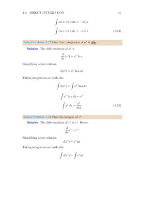
Solved Problem 1.17 Find the integral of c.
Solution Let cx is a function whose differentiation with respect to x gives
constant c. Hence
d
dx
(cx) = c
d(cx) = c dx
Z
d(cx) =
Z
c dx
Z
c dx = cx (1.13)
If c = 1 then Z
1 dx = x (1.14)
R
c dx = cx This type of integral gives area as output where c is offset
value about x-axis, or we can say that it is y-axis value. Note that, in
derivative, coefficient of x is called line slope. Let dx is very small element
along the x-axis such that
dx = xi+1 − xi
and it is distributed in [1, 4]. If dx = 0.25 then there shall be 12 partitions
in [1, 4] with points x0 to x12. The length between points x = 1 and x = 4 is
sum length of these twelve partitions as
x
y
x0 x2 x4 x6 x8 x10 x12
x1 x3 x5 x7 x9 x11
dx1 dx12
l = dx1 + dx2 + . . . + dx12 = 0.25 + 0.25 + . . . + 0.25 (12 times)
This gives l = 3. In integral form we have
Z
c dx = cx

which is continuous from x = −∞ to x = ∞.
x
y
c
x0 x2 x4 x6 x8 x10 x12
x1 x3 x5 x7 x9 x11
dx1 dx12
As this gives us area, so we can get the area x ∈ [1, 4], we have
A = c × 4 − c × 1 = c × 3 = 3c
This is area which will depend on the value of c. We knew that if A = lb is
area of rectangle of length l and width b, and if width of the rectangle is 1
unit then area of that rectangle is equal to the length of the rectangle, i.e.
A = l × 1 = l. It means, integral can also be used as line integral.
1
1 2 3 4
x
y
c
If c = 1, l = 3 which is exactly the length of line segment. Therefore, this
integral is called line integral if c = 1.
1
1 2 3 4
x
y
c = 1
1 2 3 4
x
y
Here, area A is exactly equivalent to the length of line l when c = 1.

40 Integration
Solved Problem 1.18 Find the integral of xn
.
Solution The differentiation of xn
is
d
dx
(xn
) = n xn−1
d(xn
) = n xn−1
dx
Z
d(xn
) =
Z
n xn−1
dx
Z
xn−1
dx =
xn
n
For nth
power of x, n is replaced by n + 1
Z
xn
dx =
xn+1
n + 1
Z
xn
dx =
xn+1
n + 1
(1.15)
Note that, if n = −1, then the term xn
shall be equal to 1/x and its in-
tegral can not be solved by using relation 1.15 as its result is unacceptable
mathematically.
Z
xn
dx

n=−1
=
x0
0
=
1
0
= ∞
In other words, the integral is divergent at n = −1 irrespective the value of
x.
Solved Problem 1.19 Find the integral of 1
x
.
Solution The differentiation of ln(x) is 1/x. Hence
d
dx
ln(x) =
1
x

d(ln(x)) =
1
x
dx
Z
d(ln(x)) =
Z
1
x
dx
Z
1
x
dx = ln(x)
Z
1
x
dx = ln(x) (1.16)
Solved Problem 1.20 Find the integral of sin(x).
Solution The differentiation of cos(x) is − sin(x). Hence
d
dx
cos(x) = − sin(x)
d[cos(x)] = − sin(x) dx
Z
d[cos(x)] =
Z
− sin(x) dx
Z
− sin(x) dx = cos(x)
Z
sin(x) dx = − cos(x) (1.17)
Similarly Z
cos(x) dx = sin(x) (1.18)

42 Integration
Solved Problem 1.21 Find the integral of tan(x).
Solution Integration of tan x can be found by using substitution method.
The integral is Z
tan x dx =
Z
sin x
cos x
dx
Now substituting cos x = t in denominator which gives − sin x dx = dt on
differentiation. Substituting these values in the above equation and its inte-
gration becomes Z
tan x dx =
Z
−
1
t
dt
On integration right hand side of above relation.
Z
tan x dx = − ln(t)
Substituting the value of t in above relation.
Z
tan(x) dx = − ln(cos x) = ln(sec x) (1.19)
Solved Problem 1.22 Find the integral of sec t.
Solution Integration of sec t can be written as
Z
sec t dt =
Z
sec t dt
Multiply and divide, right hand side of above equation by sec t + tan t
Z
sec t dt =
Z
sec t

sec t + tan t
sec t + tan t

dt
=
Z
sec2
t + sec t tan t
sec t + tan t
dt
Now substitute sec t + tan t = u and (sec t tan t + sec2
t) dt = du in above
relation
Z
sec t dt =
Z
1
u
du
= ln |u|

Basic Integral Calculus

More Related Content

What's hot

Similar to Basic Integral Calculus

More from Arun Umrao

Recently uploaded

Basic Integral Calculus