This document is an introduction to Scilab, focusing on its core functionalities and arithmetic operations. It includes detailed sections on arithmetic keywords, core keywords, and various mathematical operations available in the software. The content is structured in a comprehensive manner, making it a useful resource for users learning to utilize Scilab effectively.

![2
Contents
I Scilab 7
1 Scilab Core 9
1.1 Introduction . . . . . . . . . . . . . . . . . . . . . . . . . . . . . . . . . . . 9
1.1.1 Everything As Matrix . . . . . . . . . . . . . . . . . . . . . . . . . 10
1.1.2 Approximate Zero . . . . . . . . . . . . . . . . . . . . . . . . . . . 11
1.1.3 Computational Error . . . . . . . . . . . . . . . . . . . . . . . . . . 11
1.2 Simple Arithmetic . . . . . . . . . . . . . . . . . . . . . . . . . . . . . . . 12
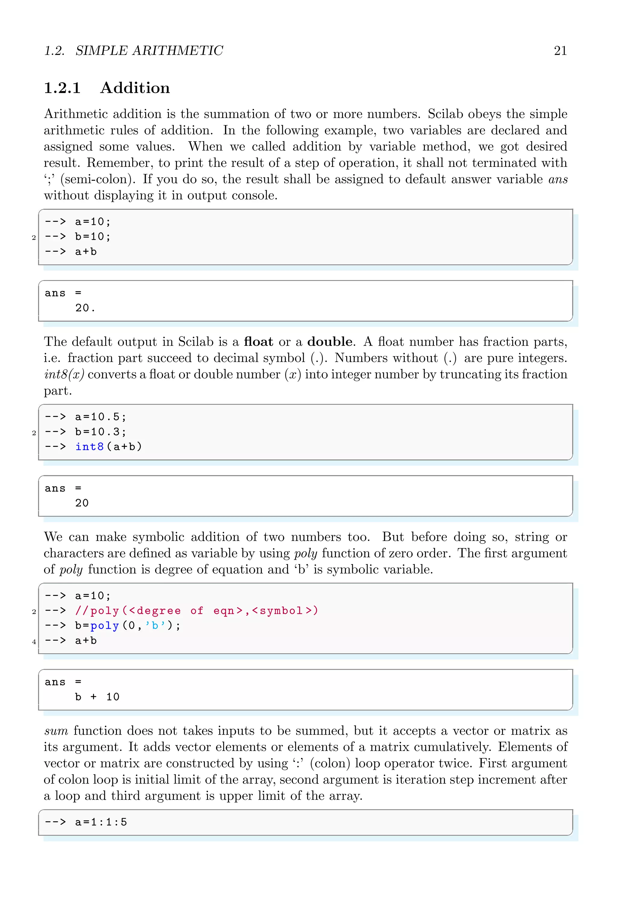
1.2.1 Addition . . . . . . . . . . . . . . . . . . . . . . . . . . . . . . . . . 13
1.2.2 Subtraction . . . . . . . . . . . . . . . . . . . . . . . . . . . . . . . 14
1.2.3 Multiplication . . . . . . . . . . . . . . . . . . . . . . . . . . . . . . 14
1.2.4 Division . . . . . . . . . . . . . . . . . . . . . . . . . . . . . . . . . 15
1.2.5 Scoping . . . . . . . . . . . . . . . . . . . . . . . . . . . . . . . . . 15
1.2.6 Square Root (sqrt) . . . . . . . . . . . . . . . . . . . . . . . . . . . 16
1.2.7 Exponent (ˆ Operator) . . . . . . . . . . . . . . . . . . . . . . . . 17
1.2.8 Algebraic Equations . . . . . . . . . . . . . . . . . . . . . . . . . . 20
1.2.9 Logarithm . . . . . . . . . . . . . . . . . . . . . . . . . . . . . . . . 21
1.2.10 Index Expression . . . . . . . . . . . . . . . . . . . . . . . . . . . . 22
1.3 Arithmetical Keywords . . . . . . . . . . . . . . . . . . . . . . . . . . . . . 25
1.3.1 Result Variable (ans) . . . . . . . . . . . . . . . . . . . . . . . . . . 25
1.3.2 Left Matrix Division () . . . . . . . . . . . . . . . . . . . . . . . . 25
1.3.3 Square Brackets ([...]) . . . . . . . . . . . . . . . . . . . . . . . . . 26
1.3.4 Element-Wise Operation . . . . . . . . . . . . . . . . . . . . . . . . 27
1.3.5 Matrix-Wise Operation . . . . . . . . . . . . . . . . . . . . . . . . 27
1.3.6 Colon (Range Operator) . . . . . . . . . . . . . . . . . . . . . . . . 27
1.3.7 Comma . . . . . . . . . . . . . . . . . . . . . . . . . . . . . . . . . 31
1.3.8 Comments . . . . . . . . . . . . . . . . . . . . . . . . . . . . . . . . 32
1.3.9 Dot . . . . . . . . . . . . . . . . . . . . . . . . . . . . . . . . . . . 32
1.3.10 Empty . . . . . . . . . . . . . . . . . . . . . . . . . . . . . . . . . . 32
1.3.11 Equal Sign . . . . . . . . . . . . . . . . . . . . . . . . . . . . . . . 33
1.3.12 global . . . . . . . . . . . . . . . . . . . . . . . . . . . . . . . . . . 33
1.3.13 Hat Symbol . . . . . . . . . . . . . . . . . . . . . . . . . . . . . . . 33
1.3.14 Less Than . . . . . . . . . . . . . . . . . . . . . . . . . . . . . . . . 34
1.3.15 Minus . . . . . . . . . . . . . . . . . . . . . . . . . . . . . . . . . . 34
1.3.16 Not . . . . . . . . . . . . . . . . . . . . . . . . . . . . . . . . . . . 34
1.3.17 Parenthesis . . . . . . . . . . . . . . . . . . . . . . . . . . . . . . . 35
1.3.18 Percent . . . . . . . . . . . . . . . . . . . . . . . . . . . . . . . . . 35
1.3.19 Plus . . . . . . . . . . . . . . . . . . . . . . . . . . . . . . . . . . . 35
1.3.20 Quote . . . . . . . . . . . . . . . . . . . . . . . . . . . . . . . . . . 35
1.3.21 Return . . . . . . . . . . . . . . . . . . . . . . . . . . . . . . . . . . 37
1.3.22 Semicolon . . . . . . . . . . . . . . . . . . . . . . . . . . . . . . . . 38
1.3.23 Forward Slash . . . . . . . . . . . . . . . . . . . . . . . . . . . . . . 39
1.3.24 Space . . . . . . . . . . . . . . . . . . . . . . . . . . . . . . . . . . 39
1.3.25 Asterisk . . . . . . . . . . . . . . . . . . . . . . . . . . . . . . . . . 39](https://image.slidesharecdn.com/scilabhelpbook1of2-220117060625/75/Scilab-help-book-1-of-2-2-2048.jpg)


![18 Scilab Core
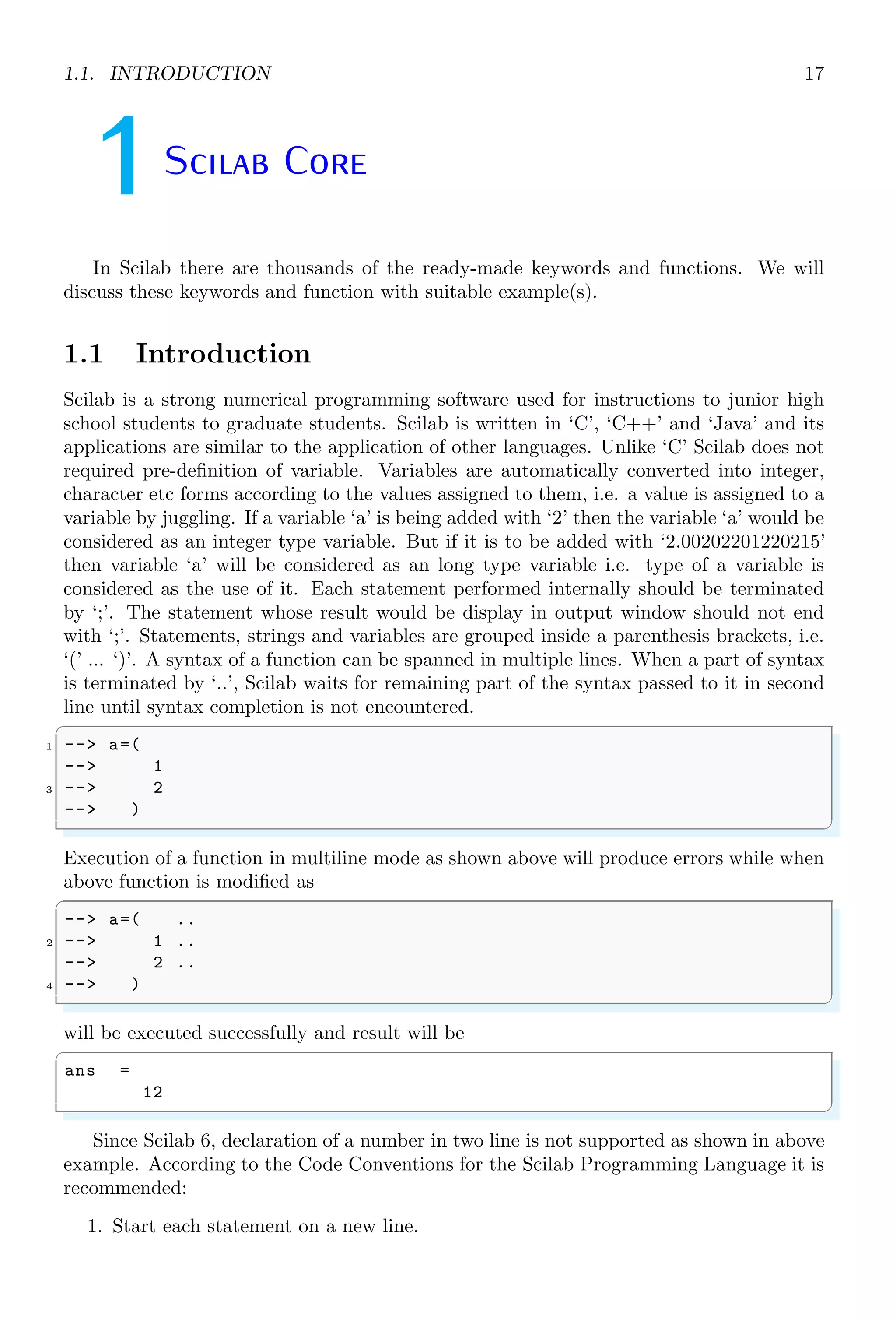
2. Write no more than one simple statement per line.
3. Break compound statements over multiple lines.
Following example uses two integers 2, 3 & ‘;’ and prints their result at output window.
✞
--> a=2; // Without pre -identification of
2 --> // variable and terminated by ’;’
--> b=3; // Without pre -identification of
4 --> // variable and terminated by ’;’
--> a+b // Sum of two variables is called
6 --> // and line does not terminated by ’;’
✌
✆
✞
ans =
5.
✌
✆
If result of an operation is not assigned to a variable, then result is automatically assigned
to ‘ans’ variable.
1.1.1 Everything As Matrix
Numerical programming by Scilab is vector or matrix based computation, therefore each
variable has a vector or matrix values. Each element of a variable is identified by its
indices. For example,
✞
--> a = 2 // one dimensional vector
2 --> a = [1,2]
--> a(1) // first element of vector
✌
✆
✞
ans =
1
✌
✆
The indices parameters inside the parentheses of variable ‘a’ may be one dimensional, two
dimensional or three dimensional.
✞
--> a(1) // One dimensional
2 --> a(1, 2) // Two dimensional
--> a(1, 2, 1)// Three dimensional
✌
✆
In the first line of above codes, first element of vector a is returned. In second line of
above codes, element at 1st
row (x) and 2nd
column (y) is returned. In the third line of
above codes, elements at 1st
row (x), 2nd
column (y) and 1st
layer (z) is returned.
✞
1 --> a = [1,2,3;5,8,4]
--> a(2,2)
3 --> b = 56;
--> b(1) // First element
5 --> b(2) // Second element . Error!!!
✌
✆](https://image.slidesharecdn.com/scilabhelpbook1of2-220117060625/75/Scilab-help-book-1-of-2-18-2048.jpg)
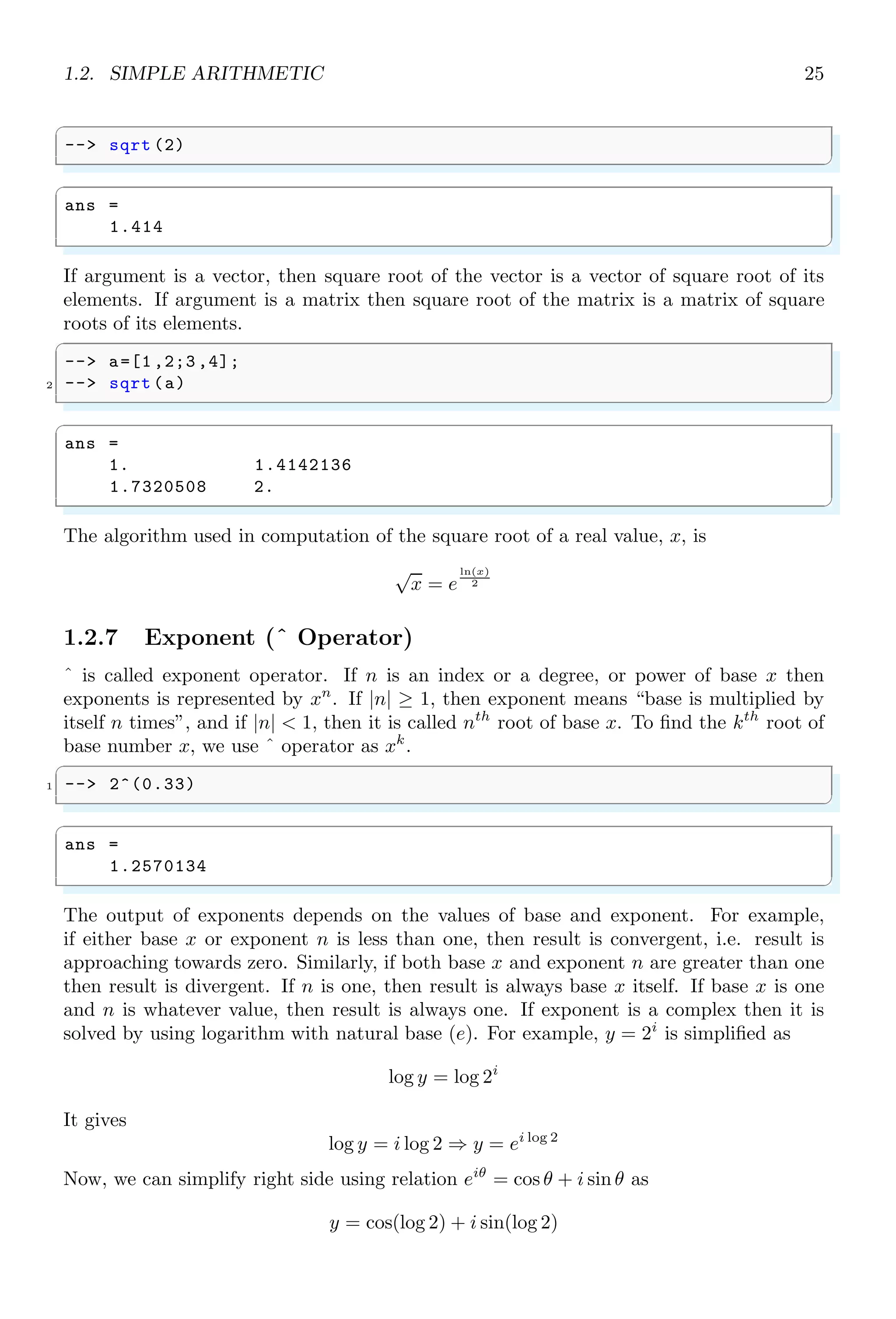
![1.2. SIMPLE ARITHMETIC 25
✞
-- sqrt (2)
✌
✆
✞
ans =
1.414
✌
✆
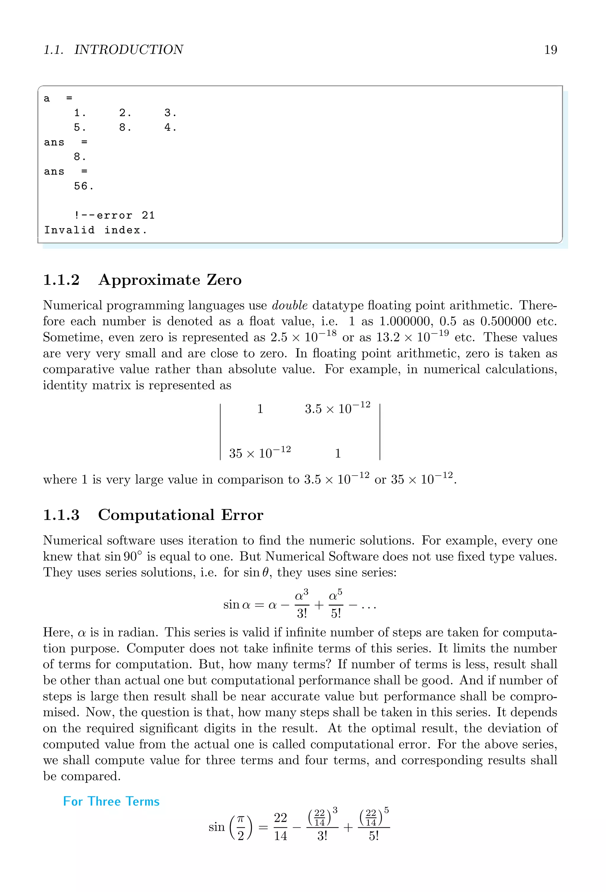
If argument is a vector, then square root of the vector is a vector of square root of its
elements. If argument is a matrix then square root of the matrix is a matrix of square
roots of its elements.
✞
-- a=[1 ,2;3 ,4];
2 -- sqrt (a)
✌
✆
✞
ans =
1. 1.4142136
1.7320508 2.
✌
✆
The algorithm used in computation of the square root of a real value, x, is
√
x = e
ln(x)
2
1.2.7 Exponent (ˆ Operator)
ˆ is called exponent operator. If n is an index or a degree, or power of base x then
exponents is represented by xn
. If |n| ≥ 1, then exponent means “base is multiplied by
itself n times”, and if |n| 1, then it is called nth
root of base x. To find the kth
root of
base number x, we use ˆ operator as xk
.
✞
1 -- 2^(0.33)
✌
✆
✞
ans =
1.2570134
✌
✆
The output of exponents depends on the values of base and exponent. For example,
if either base x or exponent n is less than one, then result is convergent, i.e. result is
approaching towards zero. Similarly, if both base x and exponent n are greater than one
then result is divergent. If n is one, then result is always base x itself. If base x is one
and n is whatever value, then result is always one. If exponent is a complex then it is
solved by using logarithm with natural base (e). For example, y = 2i
is simplified as
log y = log 2i
It gives
log y = i log 2 ⇒ y = ei log 2
Now, we can simplify right side using relation eiθ
= cos θ + i sin θ as
y = cos(log 2) + i sin(log 2)](https://image.slidesharecdn.com/scilabhelpbook1of2-220117060625/75/Scilab-help-book-1-of-2-43-2048.jpg)
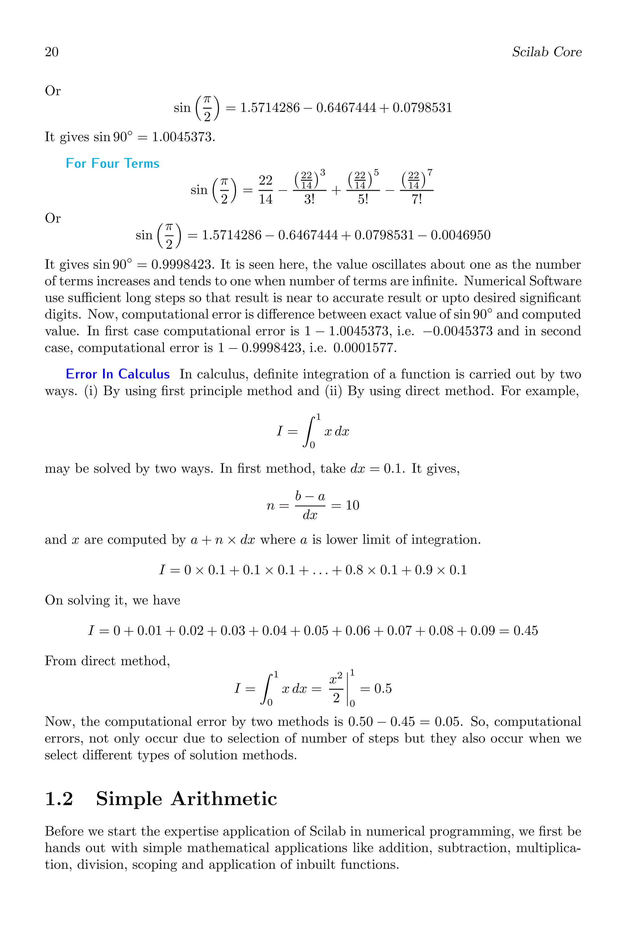
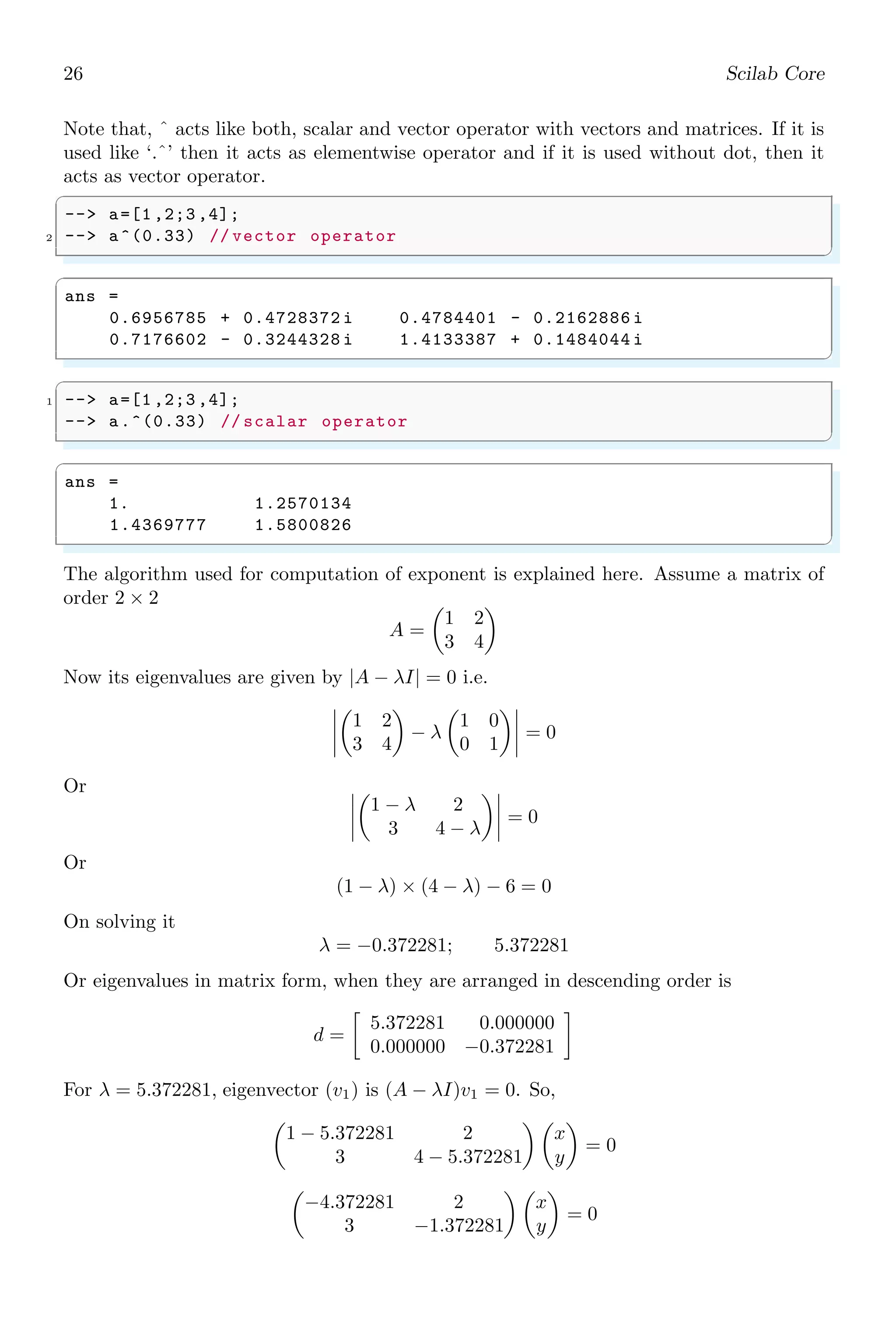
![26 Scilab Core
Note that, ˆ acts like both, scalar and vector operator with vectors and matrices. If it is
used like ‘.ˆ’ then it acts as elementwise operator and if it is used without dot, then it
acts as vector operator.
✞
-- a=[1 ,2;3 ,4];
2 -- a^(0.33) // vector operator
✌
✆
✞
ans =
0.6956785 + 0.4728372 i 0.4784401 - 0.2162886 i
0.7176602 - 0.3244328 i 1.4133387 + 0.1484044 i
✌
✆
✞
1 -- a=[1 ,2;3 ,4];
-- a.^(0.33) // scalar operator
✌
✆
✞
ans =
1. 1.2570134
1.4369777 1.5800826
✌
✆
The algorithm used for computation of exponent is explained here. Assume a matrix of
order 2 × 2
A =
1 2
3 4
Now its eigenvalues are given by |A − λI| = 0 i.e.](https://image.slidesharecdn.com/scilabhelpbook1of2-220117060625/75/Scilab-help-book-1-of-2-44-2048.jpg)
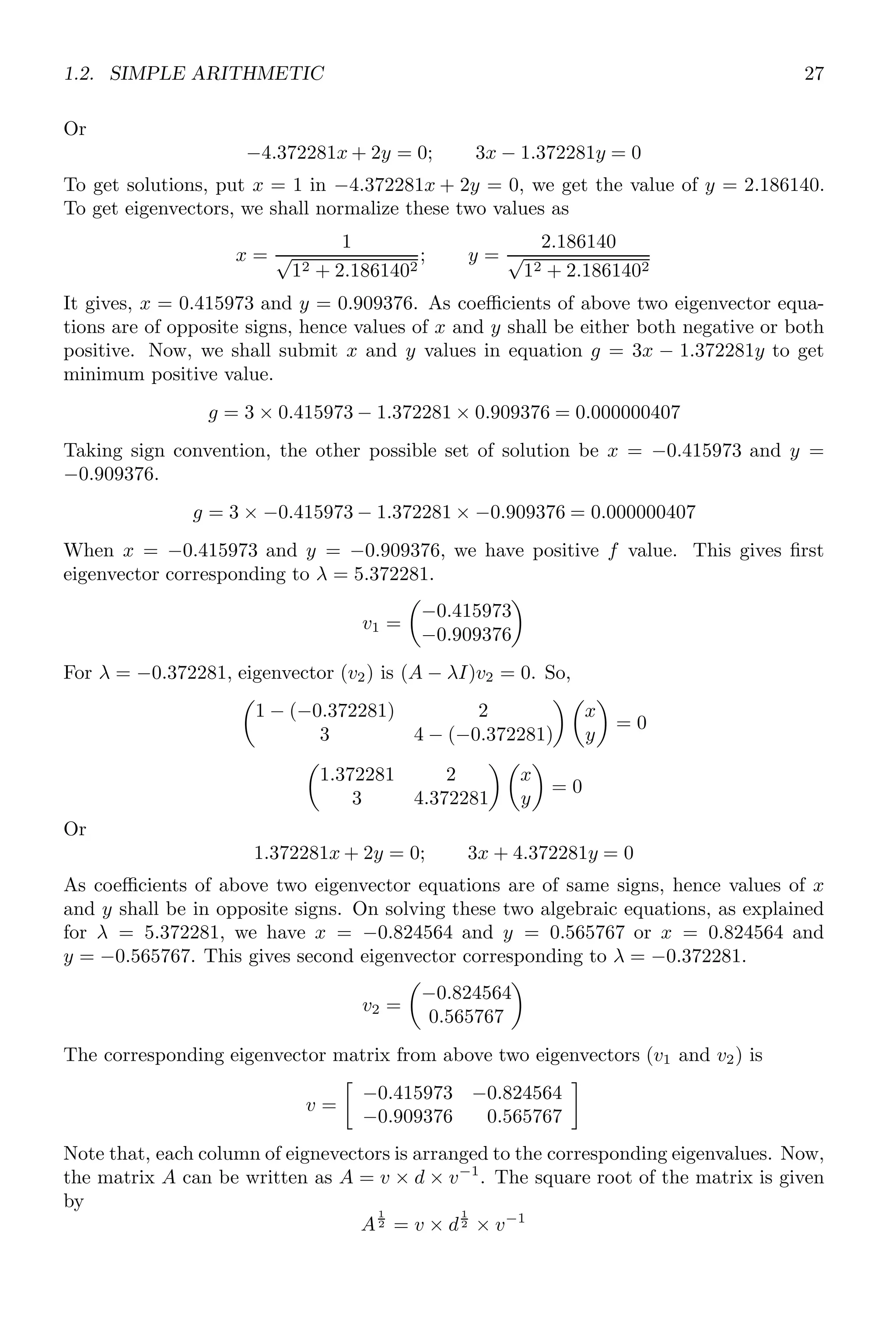
![28 Scilab Core
1.2.8 Algebraic Equations
Algebraic equations are those equations in which an unknown variable is in linear addition
or in linear subtraction in different degrees. Numerical coefficients are multiplied with
each terms to give a suitable relation for the unknown variable. To form a linear equation,
first define the variable.
✞
1 -- x=poly (0,’x’);
-- f=2*x^2+2
✌
✆
f =
2 + 2x2
This algebraic equation is in symbolic form. All the algebraic function may be applicable
to this equation. In the following example, function roots() is used to algebraic equation
f to gets its all roots.
✞
-- x=poly (0,’x’);
2 -- f=2*x ^2+2;
-- roots(f)
✌
✆
✞
ans =
i
- i
✌
✆
Division of polynomials by a number or by a symbol can also be performed. Note that it
returns only quotient of the division.
✞
1 -- x=poly (0,’x’);// returns only degree 1 polynomial
-- f=2*x ^2+2;
3 -- pdiv (f,x),
✌
✆
✞
ans =
2x
✌
✆
LCM (Least Common Multiplier) and HCF (Highest Common Factor) of two algebraic
functions can also applicable with the algebraic equations.
✞
-- x=poly (0,’x’);
2 -- f=2*x ^2+2;
-- lcm([f,x])
✌
✆
✞
ans =
3
2x + 2x
✌
✆](https://image.slidesharecdn.com/scilabhelpbook1of2-220117060625/75/Scilab-help-book-1-of-2-62-2048.jpg)
![1.2. SIMPLE ARITHMETIC 29
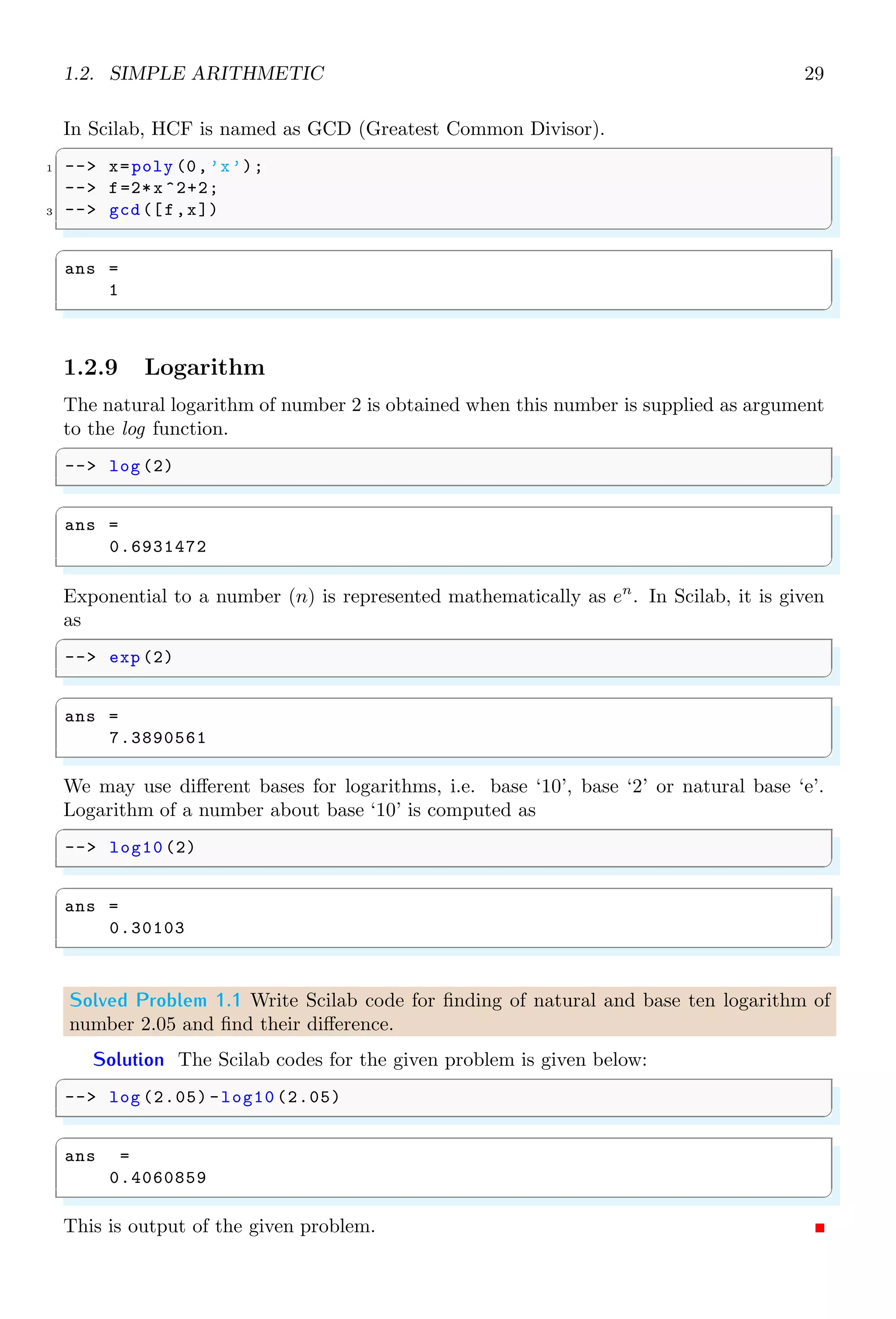
In Scilab, HCF is named as GCD (Greatest Common Divisor).
✞
1 -- x=poly (0,’x’);
-- f=2*x ^2+2;
3 -- gcd([f,x])
✌
✆
✞
ans =
1
✌
✆
1.2.9 Logarithm
The natural logarithm of number 2 is obtained when this number is supplied as argument
to the log function.
✞
-- log (2)
✌
✆
✞
ans =
0.6931472
✌
✆
Exponential to a number (n) is represented mathematically as en
. In Scilab, it is given
as
✞
-- exp (2)
✌
✆
✞
ans =
7.3890561
✌
✆
We may use different bases for logarithms, i.e. base ‘10’, base ‘2’ or natural base ‘e’.
Logarithm of a number about base ‘10’ is computed as
✞
-- log10 (2)
✌
✆
✞
ans =
0.30103
✌
✆
Solved Problem 1.1 Write Scilab code for finding of natural and base ten logarithm of
number 2.05 and find their difference.
Solution The Scilab codes for the given problem is given below:
✞
-- log (2.05) -log10 (2.05)
✌
✆
✞
ans =
0.4060859
✌
✆
This is output of the given problem.](https://image.slidesharecdn.com/scilabhelpbook1of2-220117060625/75/Scilab-help-book-1-of-2-63-2048.jpg)
![30 Scilab Core
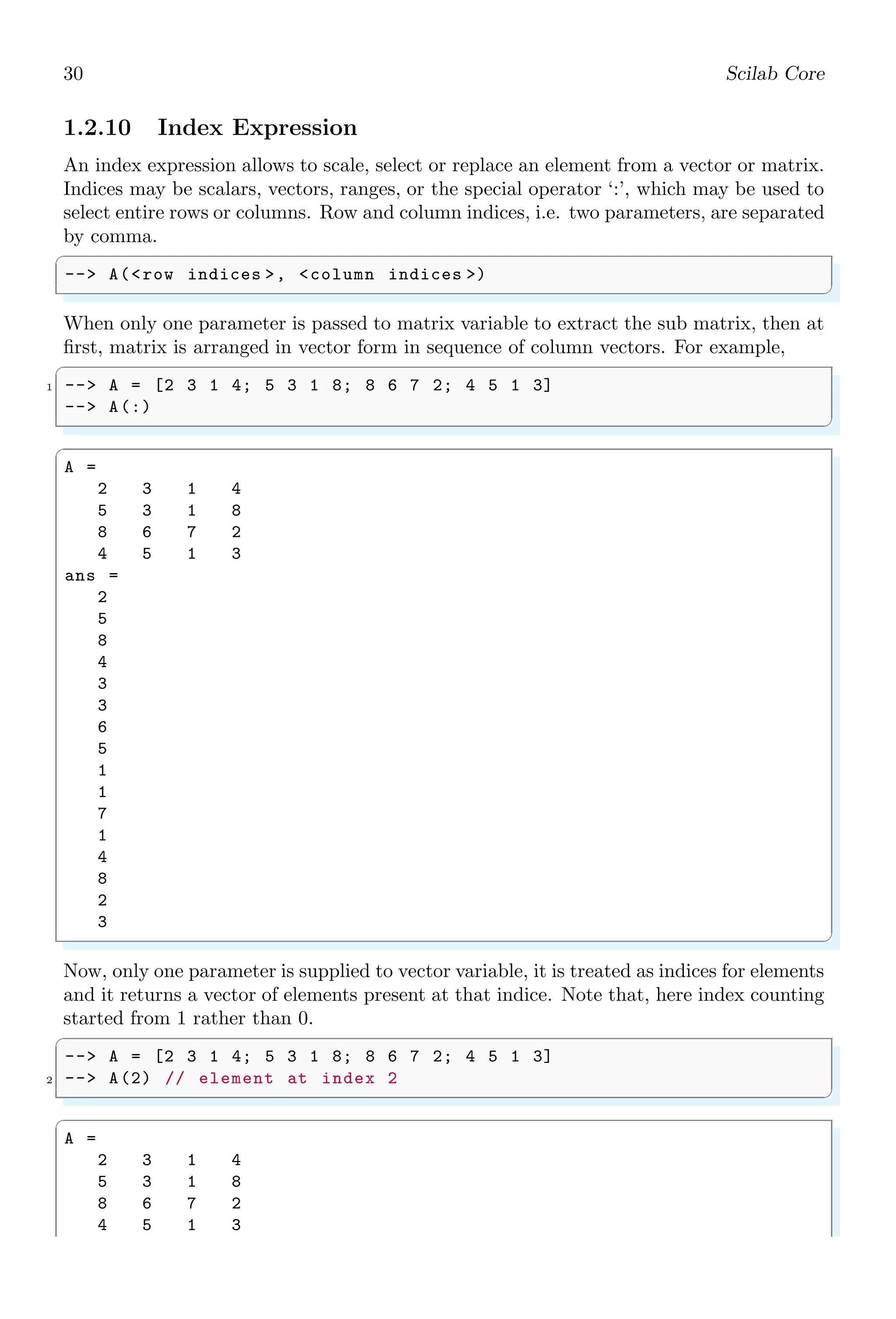
1.2.10 Index Expression
An index expression allows to scale, select or replace an element from a vector or matrix.
Indices may be scalars, vectors, ranges, or the special operator ‘:’, which may be used to
select entire rows or columns. Row and column indices, i.e. two parameters, are separated
by comma.
✞
-- A(row indices , column indices )
✌
✆
When only one parameter is passed to matrix variable to extract the sub matrix, then at
first, matrix is arranged in vector form in sequence of column vectors. For example,
✞
1 -- A = [2 3 1 4; 5 3 1 8; 8 6 7 2; 4 5 1 3]
-- A(:)
✌
✆
✞
A =
2 3 1 4
5 3 1 8
8 6 7 2
4 5 1 3
ans =
2
5
8
4
3
3
6
5
1
1
7
1
4
8
2
3
✌
✆
Now, only one parameter is supplied to vector variable, it is treated as indices for elements
and it returns a vector of elements present at that indice. Note that, here index counting
started from 1 rather than 0.
✞
-- A = [2 3 1 4; 5 3 1 8; 8 6 7 2; 4 5 1 3]
2 -- A(2) // element at index 2
✌
✆
✞
A =
2 3 1 4
5 3 1 8
8 6 7 2
4 5 1 3](https://image.slidesharecdn.com/scilabhelpbook1of2-220117060625/75/Scilab-help-book-1-of-2-64-2048.jpg)
![1.2. SIMPLE ARITHMETIC 31
ans =
5
✌
✆
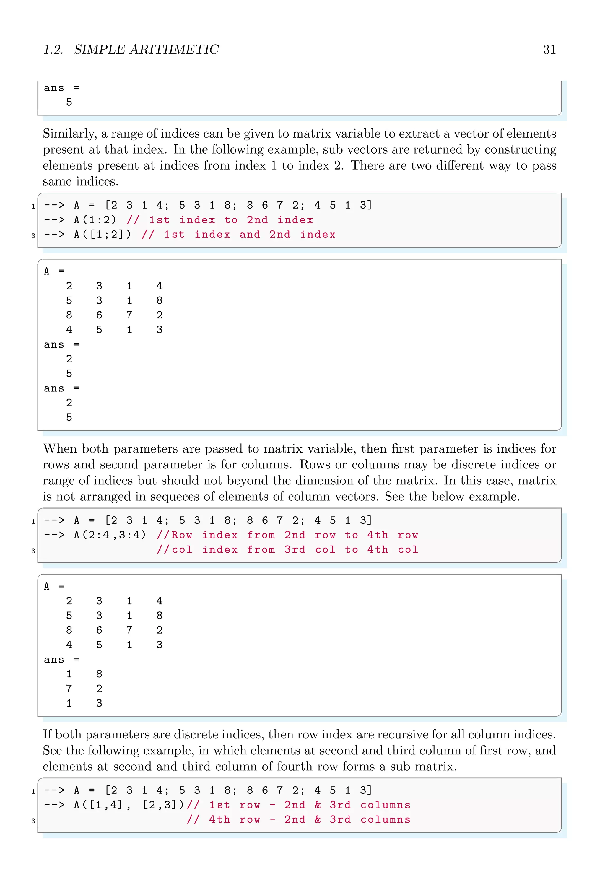
Similarly, a range of indices can be given to matrix variable to extract a vector of elements
present at that index. In the following example, sub vectors are returned by constructing
elements present at indices from index 1 to index 2. There are two different way to pass
same indices.
✞
1 -- A = [2 3 1 4; 5 3 1 8; 8 6 7 2; 4 5 1 3]
-- A(1:2) // 1st index to 2nd index
3 -- A([1;2]) // 1st index and 2nd index
✌
✆
✞
A =
2 3 1 4
5 3 1 8
8 6 7 2
4 5 1 3
ans =
2
5
ans =
2
5
✌
✆
When both parameters are passed to matrix variable, then first parameter is indices for
rows and second parameter is for columns. Rows or columns may be discrete indices or
range of indices but should not beyond the dimension of the matrix. In this case, matrix
is not arranged in sequeces of elements of column vectors. See the below example.
✞
1 -- A = [2 3 1 4; 5 3 1 8; 8 6 7 2; 4 5 1 3]
-- A(2:4 ,3:4) // Row index from 2nd row to 4th row
3 // col index from 3rd col to 4th col
✌
✆
✞
A =
2 3 1 4
5 3 1 8
8 6 7 2
4 5 1 3
ans =
1 8
7 2
1 3
✌
✆
If both parameters are discrete indices, then row index are recursive for all column indices.
See the following example, in which elements at second and third column of first row, and
elements at second and third column of fourth row forms a sub matrix.
✞
1 -- A = [2 3 1 4; 5 3 1 8; 8 6 7 2; 4 5 1 3]
-- A([1,4], [2 ,3])// 1st row - 2nd 3rd columns
3 // 4th row - 2nd 3rd columns
✌
✆](https://image.slidesharecdn.com/scilabhelpbook1of2-220117060625/75/Scilab-help-book-1-of-2-65-2048.jpg)
![32 Scilab Core
✞
A =
2 3 1 4
5 3 1 8
8 6 7 2
4 5 1 3
ans =
3 1
5 1
✌
✆
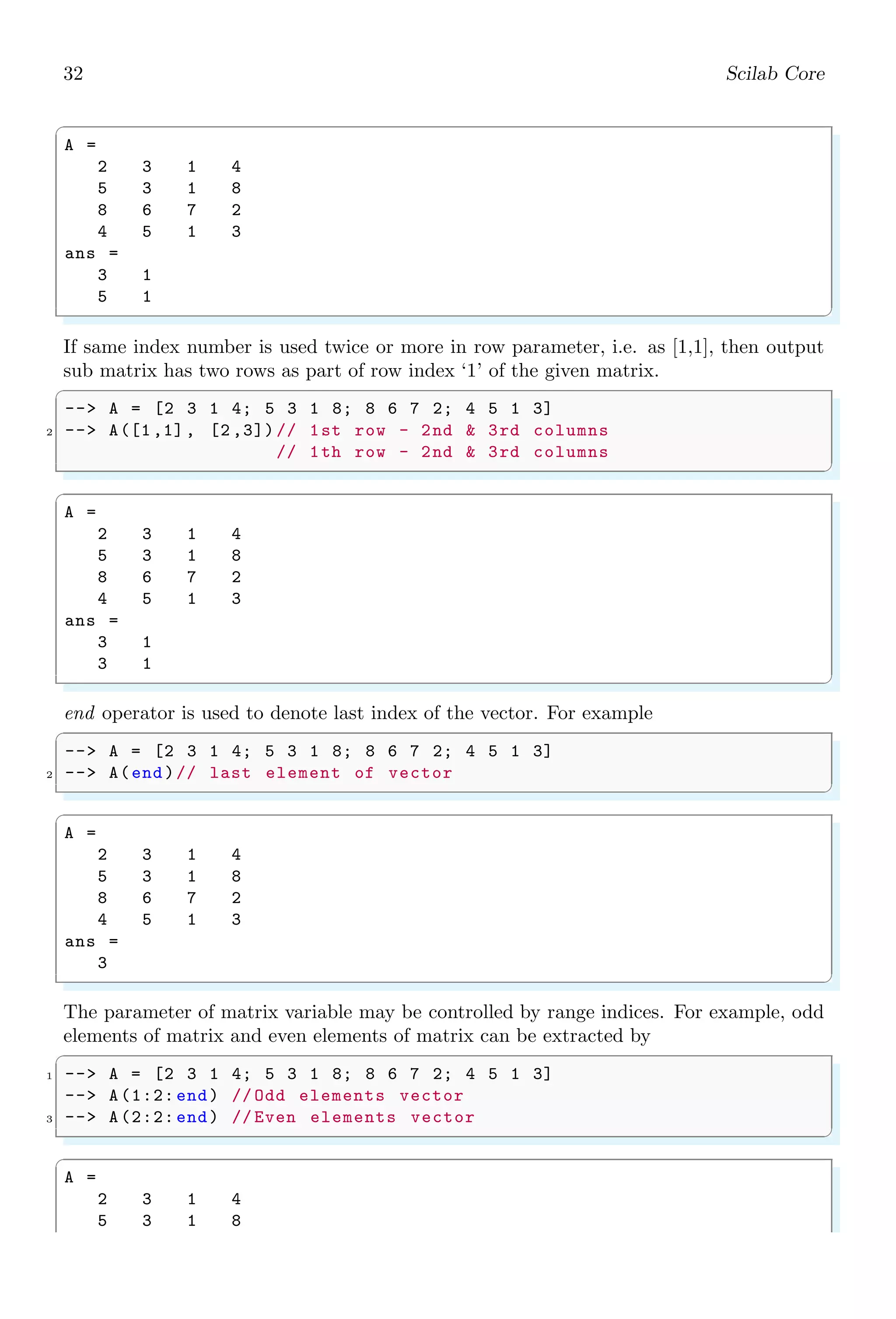
If same index number is used twice or more in row parameter, i.e. as [1,1], then output
sub matrix has two rows as part of row index ‘1’ of the given matrix.
✞
-- A = [2 3 1 4; 5 3 1 8; 8 6 7 2; 4 5 1 3]
2 -- A([1,1], [2 ,3])// 1st row - 2nd 3rd columns
// 1th row - 2nd 3rd columns
✌
✆
✞
A =
2 3 1 4
5 3 1 8
8 6 7 2
4 5 1 3
ans =
3 1
3 1
✌
✆
end operator is used to denote last index of the vector. For example
✞
-- A = [2 3 1 4; 5 3 1 8; 8 6 7 2; 4 5 1 3]
2 -- A(end)// last element of vector
✌
✆
✞
A =
2 3 1 4
5 3 1 8
8 6 7 2
4 5 1 3
ans =
3
✌
✆
The parameter of matrix variable may be controlled by range indices. For example, odd
elements of matrix and even elements of matrix can be extracted by
✞
1 -- A = [2 3 1 4; 5 3 1 8; 8 6 7 2; 4 5 1 3]
-- A(1:2: end) // Odd elements vector
3 -- A(2:2: end) // Even elements vector
✌
✆
✞
A =
2 3 1 4
5 3 1 8](https://image.slidesharecdn.com/scilabhelpbook1of2-220117060625/75/Scilab-help-book-1-of-2-66-2048.jpg)
![1.3. ARITHMETICAL KEYWORDS 33
8 6 7 2
4 5 1 3
ans =
2 8 3 6 1 7 4 2
ans =
5 4 3 5 1 1 8 3
✌
✆
1.3 Arithmetical Keywords
Followings are the main keywords used in Scilab. The key by key explanation is given
below.
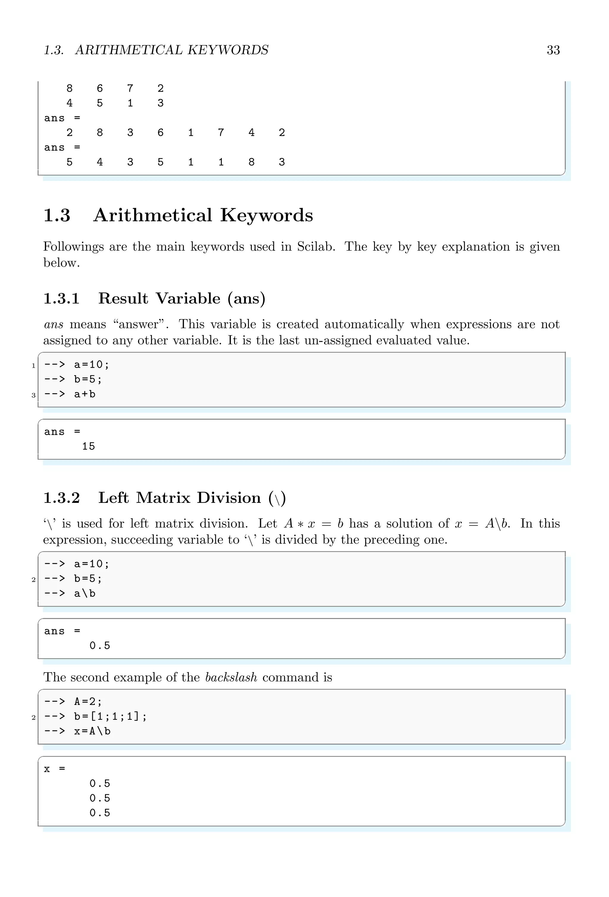
1.3.1 Result Variable (ans)
ans means “answer”. This variable is created automatically when expressions are not
assigned to any other variable. It is the last un-assigned evaluated value.
✞
1 -- a=10;
-- b=5;
3 -- a+b
✌
✆
✞
ans =
15
✌
✆
1.3.2 Left Matrix Division ()
‘’ is used for left matrix division. Let A ∗ x = b has a solution of x = Ab. In this
expression, succeeding variable to ‘’ is divided by the preceding one.
✞
-- a=10;
2 -- b=5;
-- ab
✌
✆
✞
ans =
0.5
✌
✆
The second example of the backslash command is
✞
-- A=2;
2 -- b=[1;1;1];
-- x=Ab
✌
✆
✞
x =
0.5
0.5
0.5
✌
✆](https://image.slidesharecdn.com/scilabhelpbook1of2-220117060625/75/Scilab-help-book-1-of-2-67-2048.jpg)
![34 Scilab Core
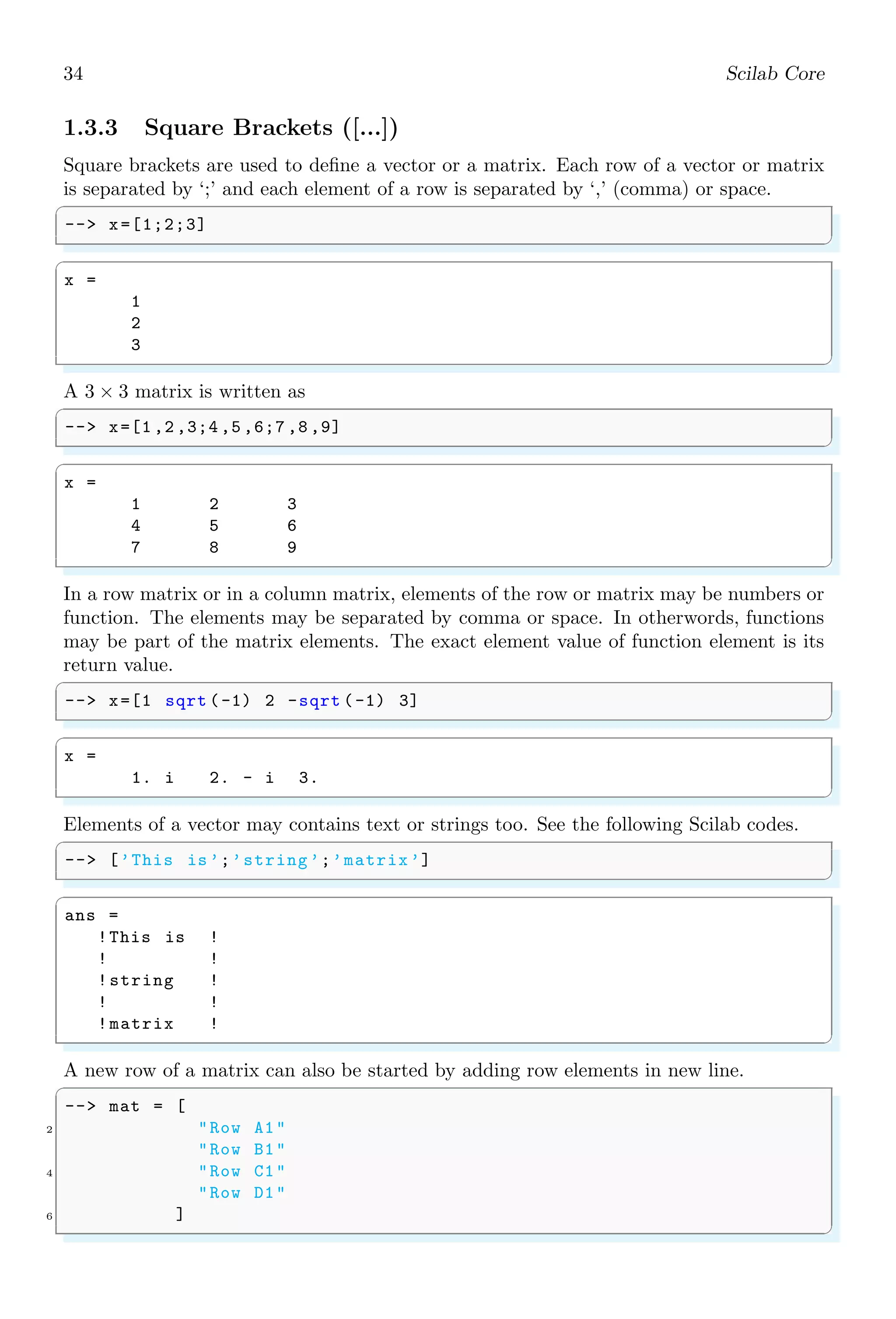
1.3.3 Square Brackets ([...])
Square brackets are used to define a vector or a matrix. Each row of a vector or matrix
is separated by ‘;’ and each element of a row is separated by ‘,’ (comma) or space.
✞
-- x=[1;2;3]
✌
✆
✞
x =
1
2
3
✌
✆
A 3 × 3 matrix is written as
✞
-- x=[1 ,2 ,3;4 ,5 ,6;7 ,8 ,9]
✌
✆
✞
x =
1 2 3
4 5 6
7 8 9
✌
✆
In a row matrix or in a column matrix, elements of the row or matrix may be numbers or
function. The elements may be separated by comma or space. In otherwords, functions
may be part of the matrix elements. The exact element value of function element is its
return value.
✞
-- x=[1 sqrt (-1) 2 -sqrt (-1) 3]
✌
✆
✞
x =
1. i 2. - i 3.
✌
✆
Elements of a vector may contains text or strings too. See the following Scilab codes.
✞
-- [’This is’;’string’;’matrix’]
✌
✆
✞
ans =
!This is !
! !
!string !
! !
!matrix !
✌
✆
A new row of a matrix can also be started by adding row elements in new line.
✞
-- mat = [
2 Row A1
Row B1
4 Row C1
Row D1
6 ]
✌
✆](https://image.slidesharecdn.com/scilabhelpbook1of2-220117060625/75/Scilab-help-book-1-of-2-68-2048.jpg)
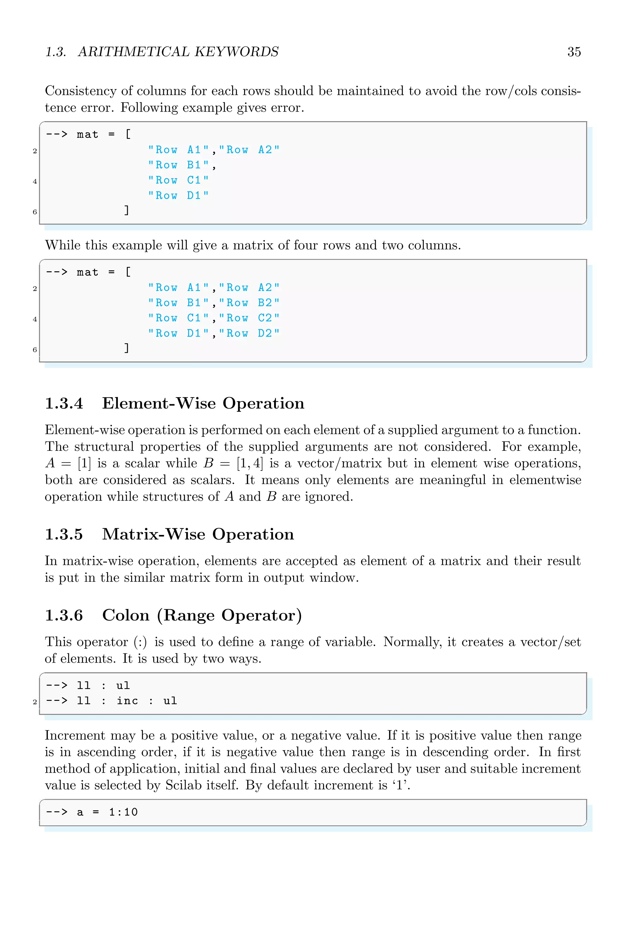
![1.3. ARITHMETICAL KEYWORDS 35
Consistency of columns for each rows should be maintained to avoid the row/cols consis-
tence error. Following example gives error.
✞
-- mat = [
2 Row A1,Row A2
Row B1,
4 Row C1
Row D1
6 ]
✌
✆
While this example will give a matrix of four rows and two columns.
✞
-- mat = [
2 Row A1,Row A2
Row B1,Row B2
4 Row C1,Row C2
Row D1,Row D2
6 ]
✌
✆
1.3.4 Element-Wise Operation
Element-wise operation is performed on each element of a supplied argument to a function.
The structural properties of the supplied arguments are not considered. For example,
A = [1] is a scalar while B = [1, 4] is a vector/matrix but in element wise operations,
both are considered as scalars. It means only elements are meaningful in elementwise
operation while structures of A and B are ignored.
1.3.5 Matrix-Wise Operation
In matrix-wise operation, elements are accepted as element of a matrix and their result
is put in the similar matrix form in output window.
1.3.6 Colon (Range Operator)
This operator (:) is used to define a range of variable. Normally, it creates a vector/set
of elements. It is used by two ways.
✞
-- ll : ul
2 -- ll : inc : ul
✌
✆
Increment may be a positive value, or a negative value. If it is positive value then range
is in ascending order, if it is negative value then range is in descending order. In first
method of application, initial and final values are declared by user and suitable increment
value is selected by Scilab itself. By default increment is ‘1’.
✞
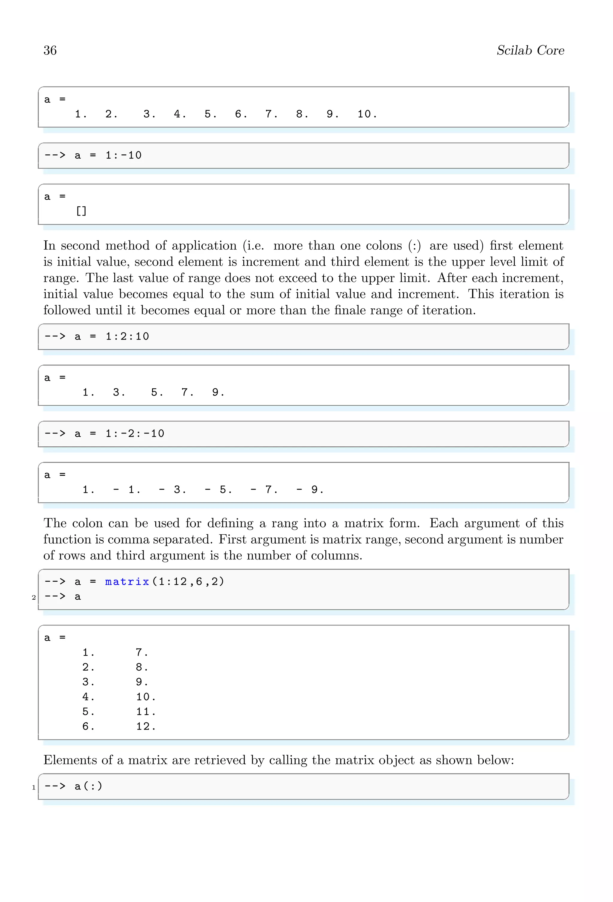
-- a = 1:10
✌
✆](https://image.slidesharecdn.com/scilabhelpbook1of2-220117060625/75/Scilab-help-book-1-of-2-69-2048.jpg)
![36 Scilab Core
✞
a =
1. 2. 3. 4. 5. 6. 7. 8. 9. 10.
✌
✆
✞
-- a = 1:-10
✌
✆
✞
a =
[]
✌
✆
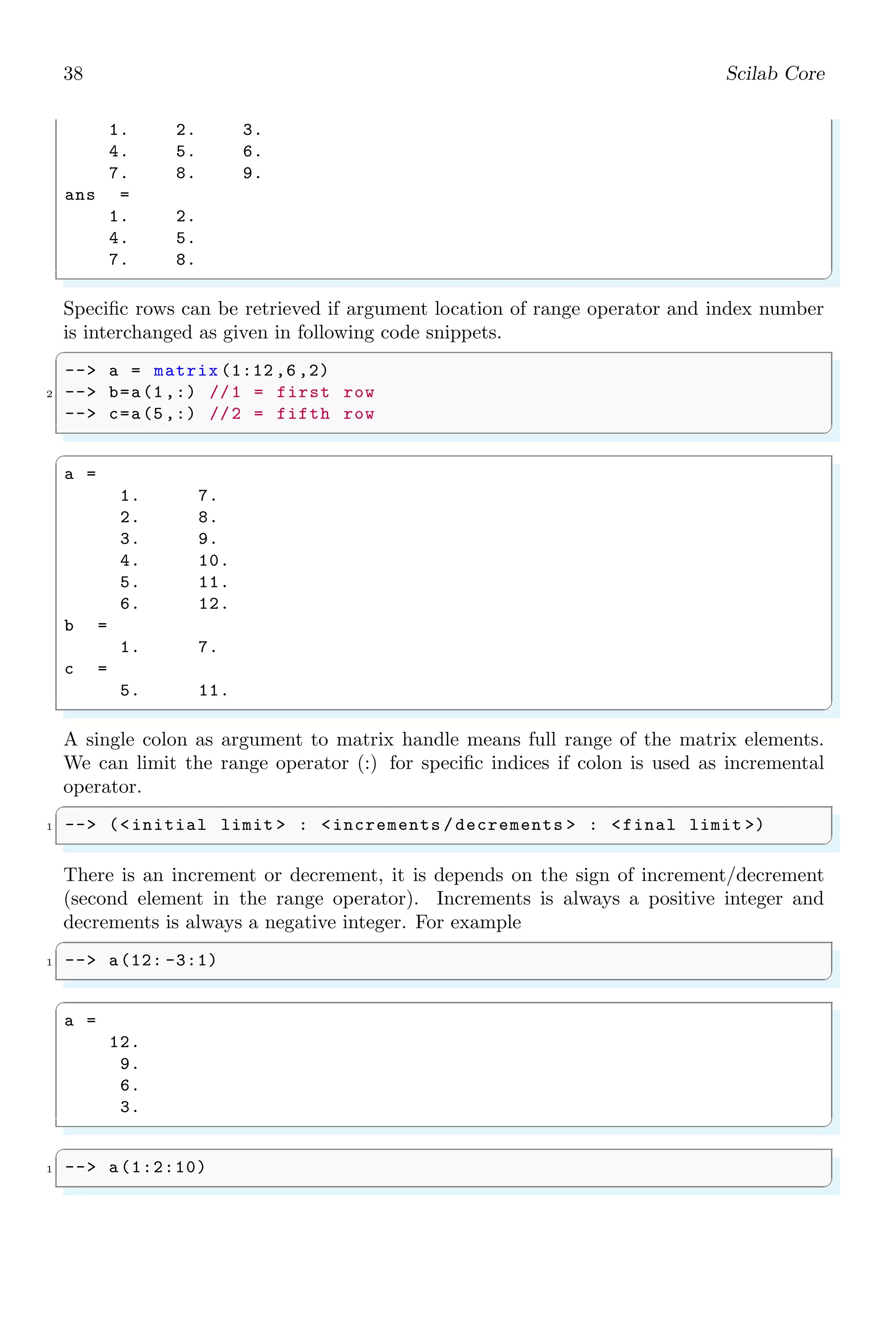
In second method of application (i.e. more than one colons (:) are used) first element
is initial value, second element is increment and third element is the upper level limit of
range. The last value of range does not exceed to the upper limit. After each increment,
initial value becomes equal to the sum of initial value and increment. This iteration is
followed until it becomes equal or more than the finale range of iteration.
✞
-- a = 1:2:10
✌
✆
✞
a =
1. 3. 5. 7. 9.
✌
✆
✞
-- a = 1:-2:-10
✌
✆
✞
a =
1. - 1. - 3. - 5. - 7. - 9.
✌
✆
The colon can be used for defining a rang into a matrix form. Each argument of this
function is comma separated. First argument is matrix range, second argument is number
of rows and third argument is the number of columns.
✞
-- a = matrix (1:12 ,6 ,2)
2 -- a
✌
✆
✞
a =
1. 7.
2. 8.
3. 9.
4. 10.
5. 11.
6. 12.
✌
✆
Elements of a matrix are retrieved by calling the matrix object as shown below:
✞
1 -- a(:)
✌
✆](https://image.slidesharecdn.com/scilabhelpbook1of2-220117060625/75/Scilab-help-book-1-of-2-70-2048.jpg)
![1.3. ARITHMETICAL KEYWORDS 37
✞
ans =
1.
2.
3.
4.
5.
6.
7.
8.
9.
10.
11.
12.
✌
✆
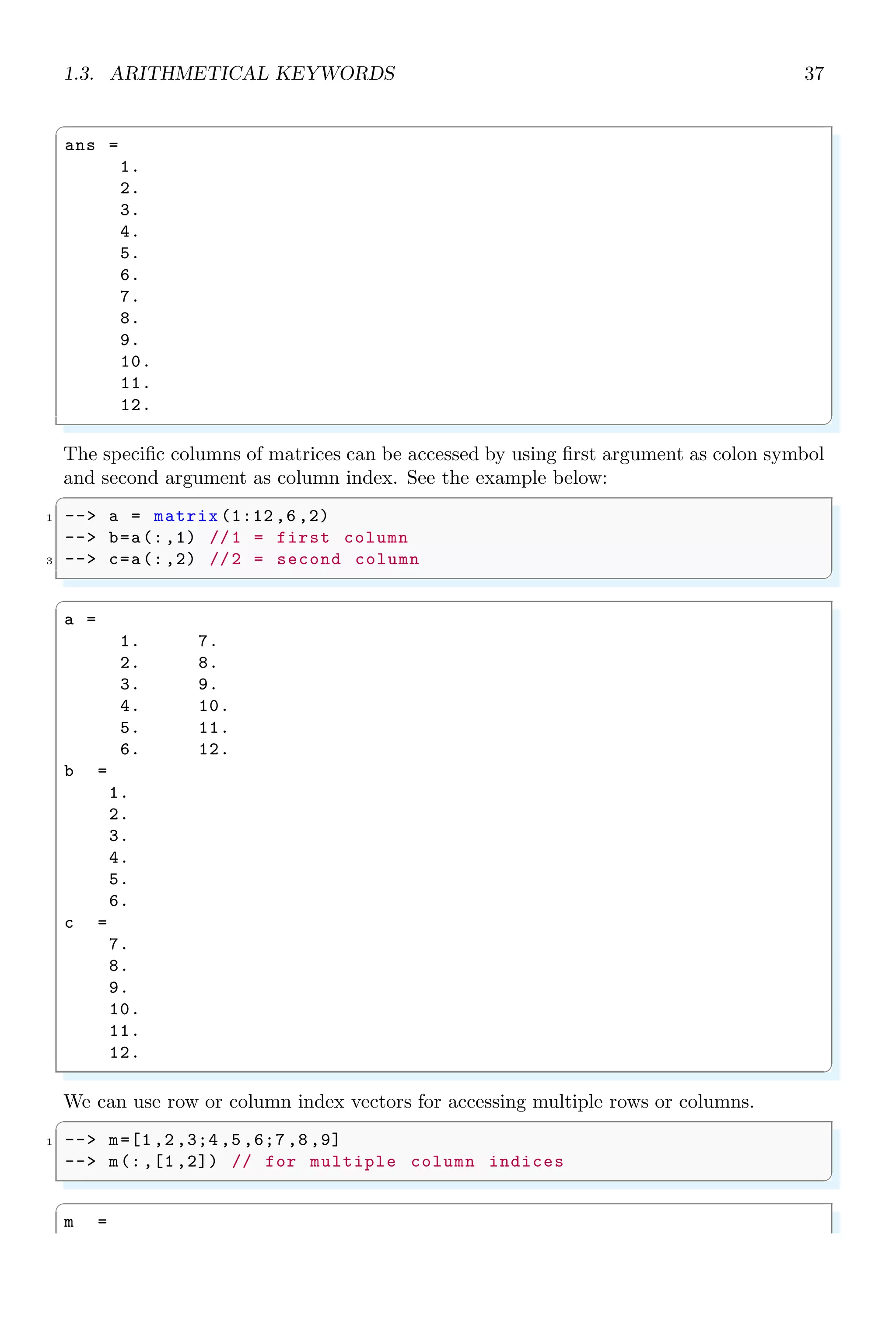
The specific columns of matrices can be accessed by using first argument as colon symbol
and second argument as column index. See the example below:
✞
1 -- a = matrix (1:12 ,6 ,2)
-- b=a(:,1) //1 = first column
3 -- c=a(:,2) //2 = second column
✌
✆
✞
a =
1. 7.
2. 8.
3. 9.
4. 10.
5. 11.
6. 12.
b =
1.
2.
3.
4.
5.
6.
c =
7.
8.
9.
10.
11.
12.
✌
✆
We can use row or column index vectors for accessing multiple rows or columns.
✞
1 -- m=[1 ,2 ,3;4 ,5 ,6;7 ,8 ,9]
-- m(: ,[1 ,2]) // for multiple column indices
✌
✆
✞
m =](https://image.slidesharecdn.com/scilabhelpbook1of2-220117060625/75/Scilab-help-book-1-of-2-71-2048.jpg)
![1.3. ARITHMETICAL KEYWORDS 39
✞
a =
1.
3.
5.
7.
9.
✌
✆
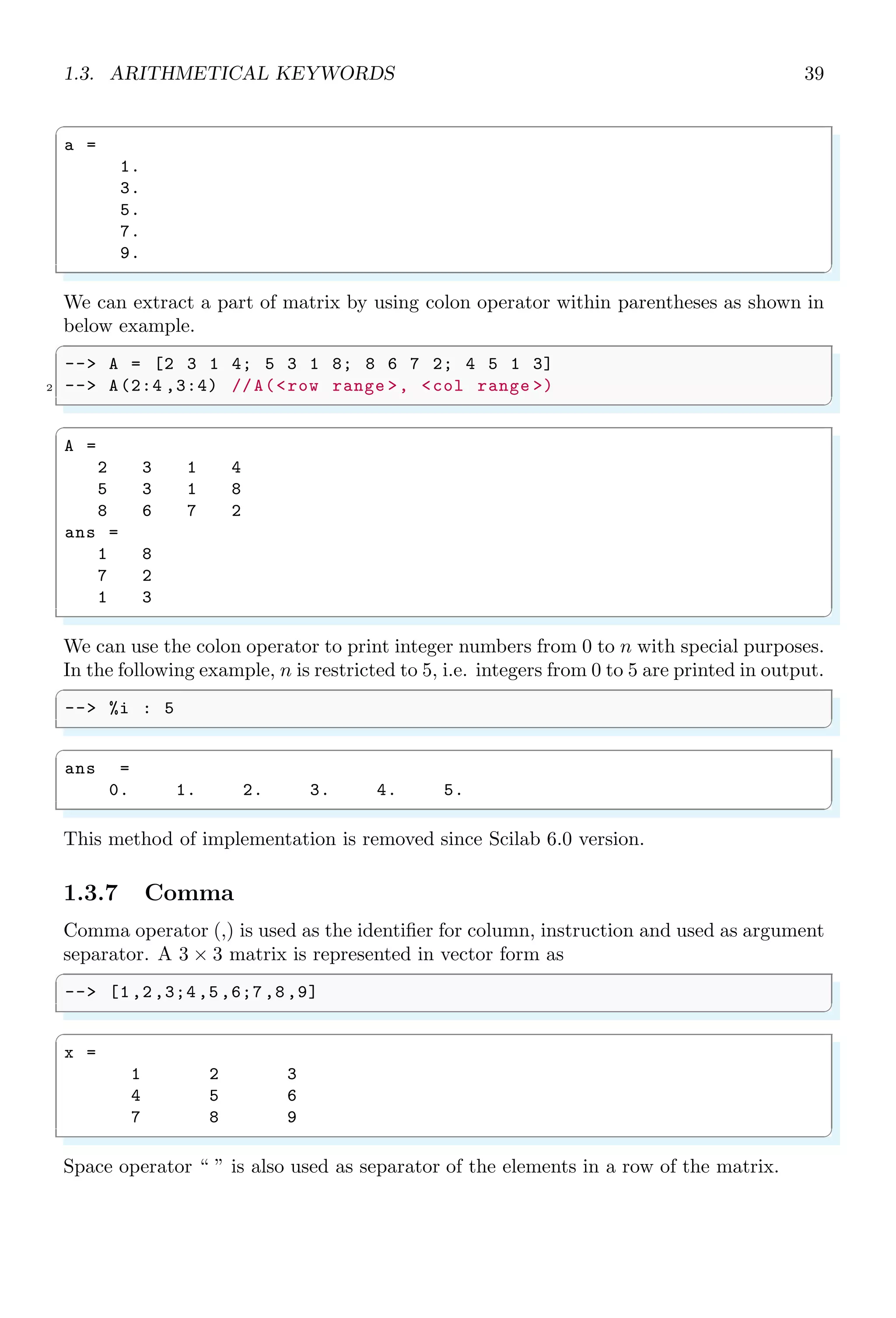
We can extract a part of matrix by using colon operator within parentheses as shown in
below example.
✞
-- A = [2 3 1 4; 5 3 1 8; 8 6 7 2; 4 5 1 3]
2 -- A(2:4 ,3:4) //A(row range , col range )
✌
✆
✞
A =
2 3 1 4
5 3 1 8
8 6 7 2
ans =
1 8
7 2
1 3
✌
✆
We can use the colon operator to print integer numbers from 0 to n with special purposes.
In the following example, n is restricted to 5, i.e. integers from 0 to 5 are printed in output.
✞
-- %i : 5
✌
✆
✞
ans =
0. 1. 2. 3. 4. 5.
✌
✆
This method of implementation is removed since Scilab 6.0 version.
1.3.7 Comma
Comma operator (,) is used as the identifier for column, instruction and used as argument
separator. A 3 × 3 matrix is represented in vector form as
✞
-- [1,2,3;4,5,6;7,8,9]
✌
✆
✞
x =
1 2 3
4 5 6
7 8 9
✌
✆
Space operator “ ” is also used as separator of the elements in a row of the matrix.](https://image.slidesharecdn.com/scilabhelpbook1of2-220117060625/75/Scilab-help-book-1-of-2-73-2048.jpg)
![40 Scilab Core
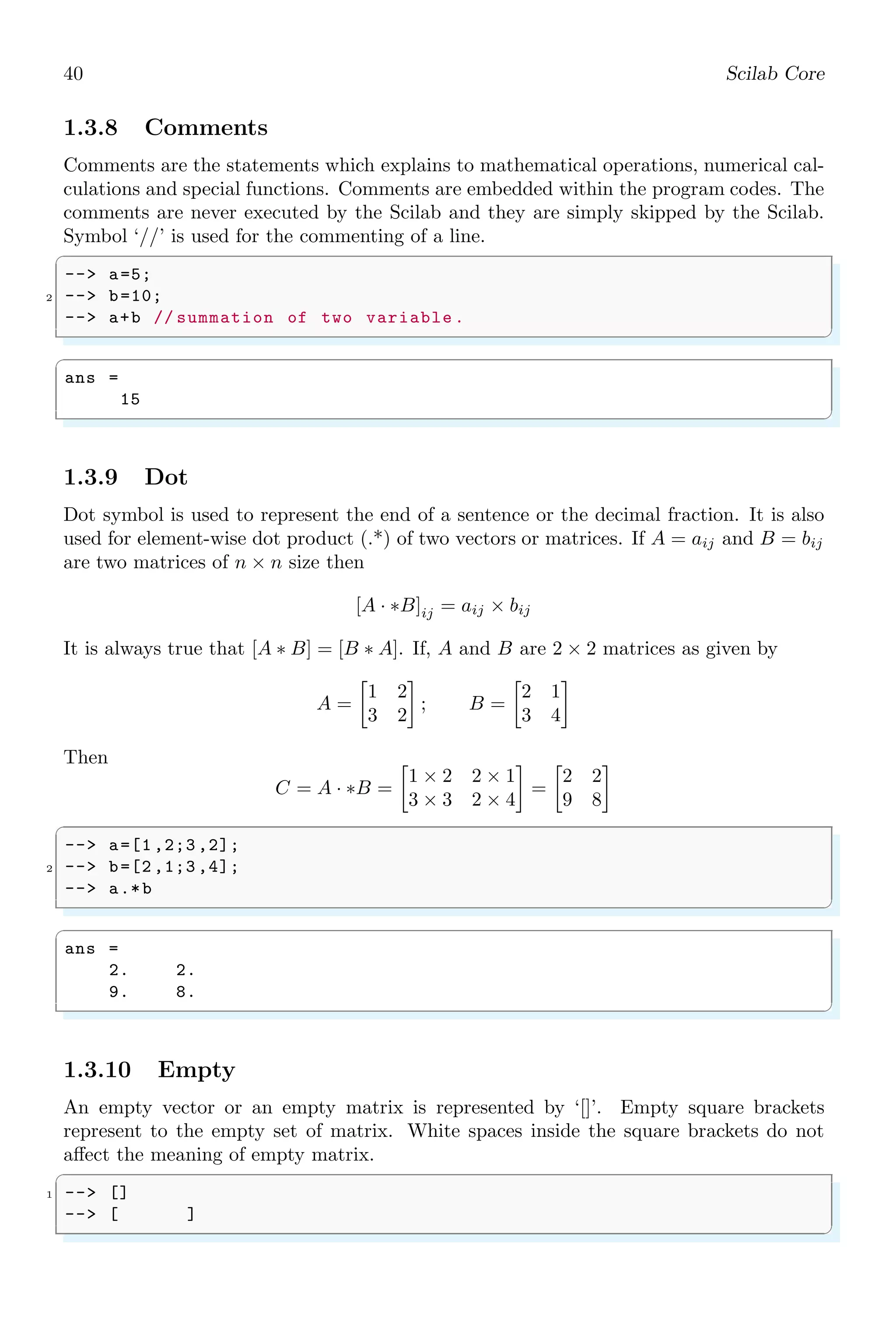
1.3.8 Comments
Comments are the statements which explains to mathematical operations, numerical cal-
culations and special functions. Comments are embedded within the program codes. The
comments are never executed by the Scilab and they are simply skipped by the Scilab.
Symbol ‘//’ is used for the commenting of a line.
✞
-- a=5;
2 -- b=10;
-- a+b // summation of two variable .
✌
✆
✞
ans =
15
✌
✆
1.3.9 Dot
Dot symbol is used to represent the end of a sentence or the decimal fraction. It is also
used for element-wise dot product (.*) of two vectors or matrices. If A = aij and B = bij
are two matrices of n × n size then
[A · ∗B]ij = aij × bij
It is always true that [A ∗ B] = [B ∗ A]. If, A and B are 2 × 2 matrices as given by
A =
1 2
3 2
; B =
2 1
3 4
Then
C = A · ∗B =
1 × 2 2 × 1
3 × 3 2 × 4
=
2 2
9 8
✞
-- a=[1 ,2;3 ,2];
2 -- b=[2 ,1;3 ,4];
-- a.*b
✌
✆
✞
ans =
2. 2.
9. 8.
✌
✆
1.3.10 Empty
An empty vector or an empty matrix is represented by ‘[]’. Empty square brackets
represent to the empty set of matrix. White spaces inside the square brackets do not
affect the meaning of empty matrix.
✞
1 -- []
-- [ ]
✌
✆](https://image.slidesharecdn.com/scilabhelpbook1of2-220117060625/75/Scilab-help-book-1-of-2-74-2048.jpg)
![1.3. ARITHMETICAL KEYWORDS 41
✞
ans =
[]
ans =
[]
✌
✆
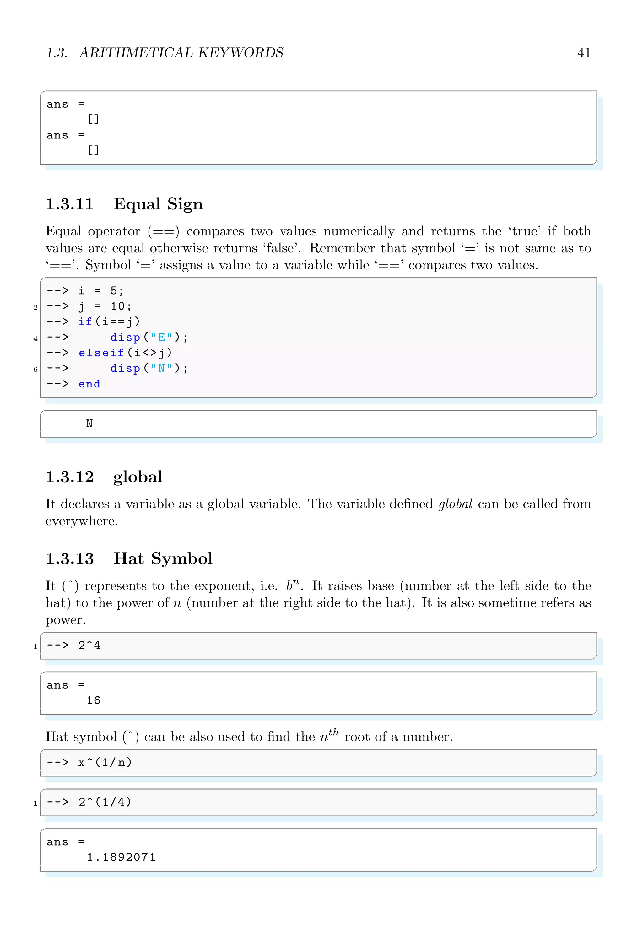
1.3.11 Equal Sign
Equal operator (==) compares two values numerically and returns the ‘true’ if both
values are equal otherwise returns ‘false’. Remember that symbol ‘=’ is not same as to
‘==’. Symbol ‘=’ assigns a value to a variable while ‘==’ compares two values.
✞
-- i = 5;
2 -- j = 10;
-- if(i==j)
4 -- disp (E);
-- elseif(ij)
6 -- disp (N);
-- end
✌
✆
✞
N
✌
✆
1.3.12 global
It declares a variable as a global variable. The variable defined global can be called from
everywhere.
1.3.13 Hat Symbol
It (ˆ) represents to the exponent, i.e. bn
. It raises base (number at the left side to the
hat) to the power of n (number at the right side to the hat). It is also sometime refers as
power.
✞
1 -- 2^4
✌
✆
✞
ans =
16
✌
✆
Hat symbol (ˆ) can be also used to find the nth
root of a number.
✞
-- x^(1/ n)
✌
✆
✞
1 -- 2^(1/4)
✌
✆
✞
ans =
1.1892071
✌
✆](https://image.slidesharecdn.com/scilabhelpbook1of2-220117060625/75/Scilab-help-book-1-of-2-75-2048.jpg)
![42 Scilab Core
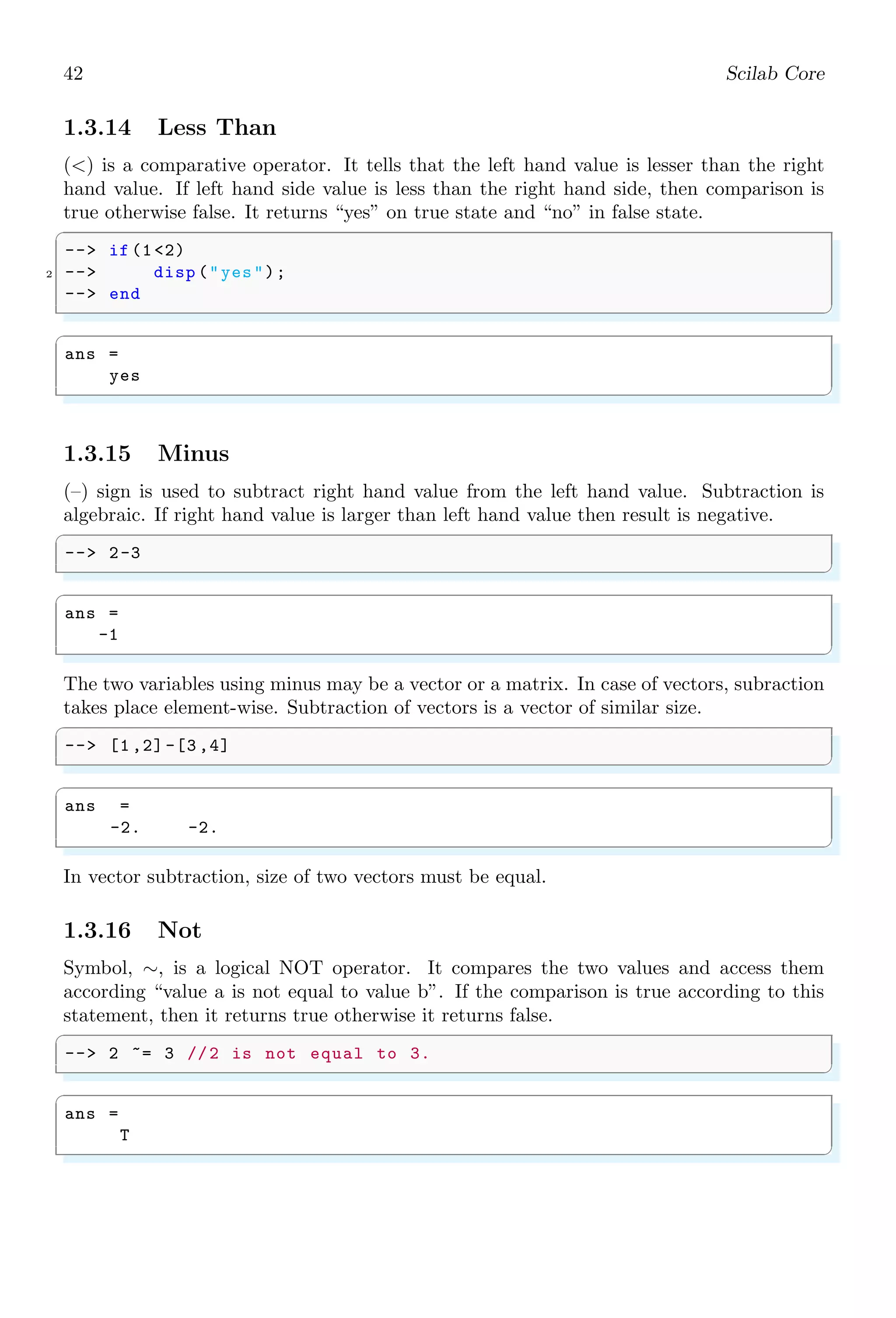
1.3.14 Less Than
() is a comparative operator. It tells that the left hand value is lesser than the right
hand value. If left hand side value is less than the right hand side, then comparison is
true otherwise false. It returns “yes” on true state and “no” in false state.
✞
-- if (12)
2 -- disp (yes);
-- end
✌
✆
✞
ans =
yes
✌
✆
1.3.15 Minus
(–) sign is used to subtract right hand value from the left hand value. Subtraction is
algebraic. If right hand value is larger than left hand value then result is negative.
✞
-- 2-3
✌
✆
✞
ans =
-1
✌
✆
The two variables using minus may be a vector or a matrix. In case of vectors, subraction
takes place element-wise. Subtraction of vectors is a vector of similar size.
✞
-- [1 ,2] -[3 ,4]
✌
✆
✞
ans =
-2. -2.
✌
✆
In vector subtraction, size of two vectors must be equal.
1.3.16 Not
Symbol, ∼, is a logical NOT operator. It compares the two values and access them
according “value a is not equal to value b”. If the comparison is true according to this
statement, then it returns true otherwise it returns false.
✞
-- 2 ~= 3 //2 is not equal to 3.
✌
✆
✞
ans =
T
✌
✆](https://image.slidesharecdn.com/scilabhelpbook1of2-220117060625/75/Scilab-help-book-1-of-2-76-2048.jpg)
![1.3. ARITHMETICAL KEYWORDS 43
1.3.17 Parenthesis
Parenthesis, i.e. ‘(...)’ brackets are used to group the statements, operations executions.
A variable or function initiated inside the parenthesis has local scope.
1.3.18 Percent
(%) is a special character. When it is prepend to string, literals are considered as with
special meaning as shown in the following table.
Symbol Meaning
%pi π
%i:n Integer from 0 to n
%i
√
−1
The functions whose names begin with % character are special functions. They are
used as primitives and used in operator’s overloading.
1.3.19 Plus
(+) is an addition operator. It returns sum of two or more values. It also concatenates
two or more strings. Its operands may be vectors, scalars or strings.
✞
-- 2+3
2 -- This is my + country .
✌
✆
✞
ans =
5
ans =
This is mycountry .
✌
✆
The two variables may be a vector or a matrices. In case of vector operands, addition
takes place element-by-element wise.
✞
--[1,2]+[3,4]
✌
✆
✞
ans =
4. 6.
✌
✆
In vector subtraction, size of two vectors must be equal.
1.3.20 Quote
There are two types of quotes, called single quotes (’) and double quotes (”). In Scilab,
single quotes and double quotes have different meaning. The contents written between
single quotes or double quotes are considered as strings. See the following example:](https://image.slidesharecdn.com/scilabhelpbook1of2-220117060625/75/Scilab-help-book-1-of-2-77-2048.jpg)
![44 Scilab Core
✞
-- x = ‘The Good Boy ’
2 -- y = The Good Boy
✌
✆
✞
x =
The Good Boy
y =
The Good Boy
✌
✆
Single quote is also used as string delimiter (”), i.e. string within string. As string
delimiter, the single quote is used in a group of twice.
✞
-- x = ‘disp (‘‘Boy ’’)’
2 -- y = disp (‘‘Boy ’’)
-- z = disp (‘‘disp (‘‘disp (‘‘Boy ’’) ’’) ’’)
✌
✆
✞
x =
disp (‘Boy ’)
y =
disp (‘Boy ’)
z =
disp (‘disp (‘disp (‘Boy ’) ’) ’)
✌
✆
Single quote is also used in mathematics, specially in matrix. If a matrix is real matrix
then single quotes converts row vector into column vector and vice-versa. See the example
given below:
✞
-- a=[1 ,2]
2 -- a’
✌
✆
✞
a =
1. 2.
ans =
1.
2.
✌
✆
If matrix is a complex matrix then (’) is a complex conjugate transpose operator. It is
used in a matrix for conjugate transpose of the matrix. It is also used as string delimiter.
Assume a complex matrix of order 2 × 2 as
A =
1 + i 2
3 2 + i
Conjugate transpose of this matrix (A) will be
A =
1 − i 3
2 2 − i](https://image.slidesharecdn.com/scilabhelpbook1of2-220117060625/75/Scilab-help-book-1-of-2-78-2048.jpg)
![1.3. ARITHMETICAL KEYWORDS 45
✞
1 -- [1+%i , 2; 3, 2+%i]’
✌
✆
✞
ans =
1. - i 3.
2. 2. - i
✌
✆
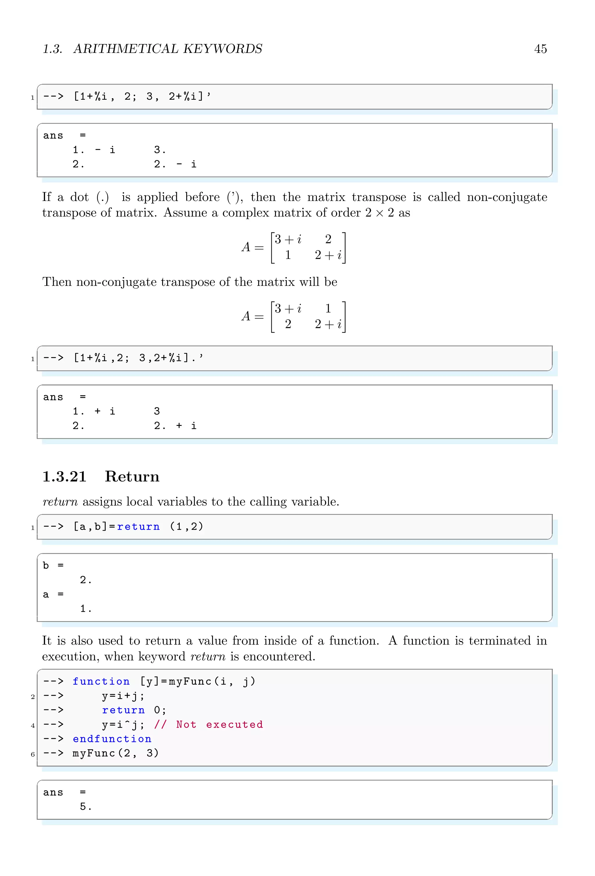
If a dot (.) is applied before (’), then the matrix transpose is called non-conjugate
transpose of matrix. Assume a complex matrix of order 2 × 2 as
A =
3 + i 2
1 2 + i
Then non-conjugate transpose of the matrix will be
A =
3 + i 1
2 2 + i
✞
1 -- [1+%i ,2; 3,2+ %i].’
✌
✆
✞
ans =
1. + i 3
2. 2. + i
✌
✆
1.3.21 Return
return assigns local variables to the calling variable.
✞
1 -- [a,b]= return (1,2)
✌
✆
✞
b =
2.
a =
1.
✌
✆
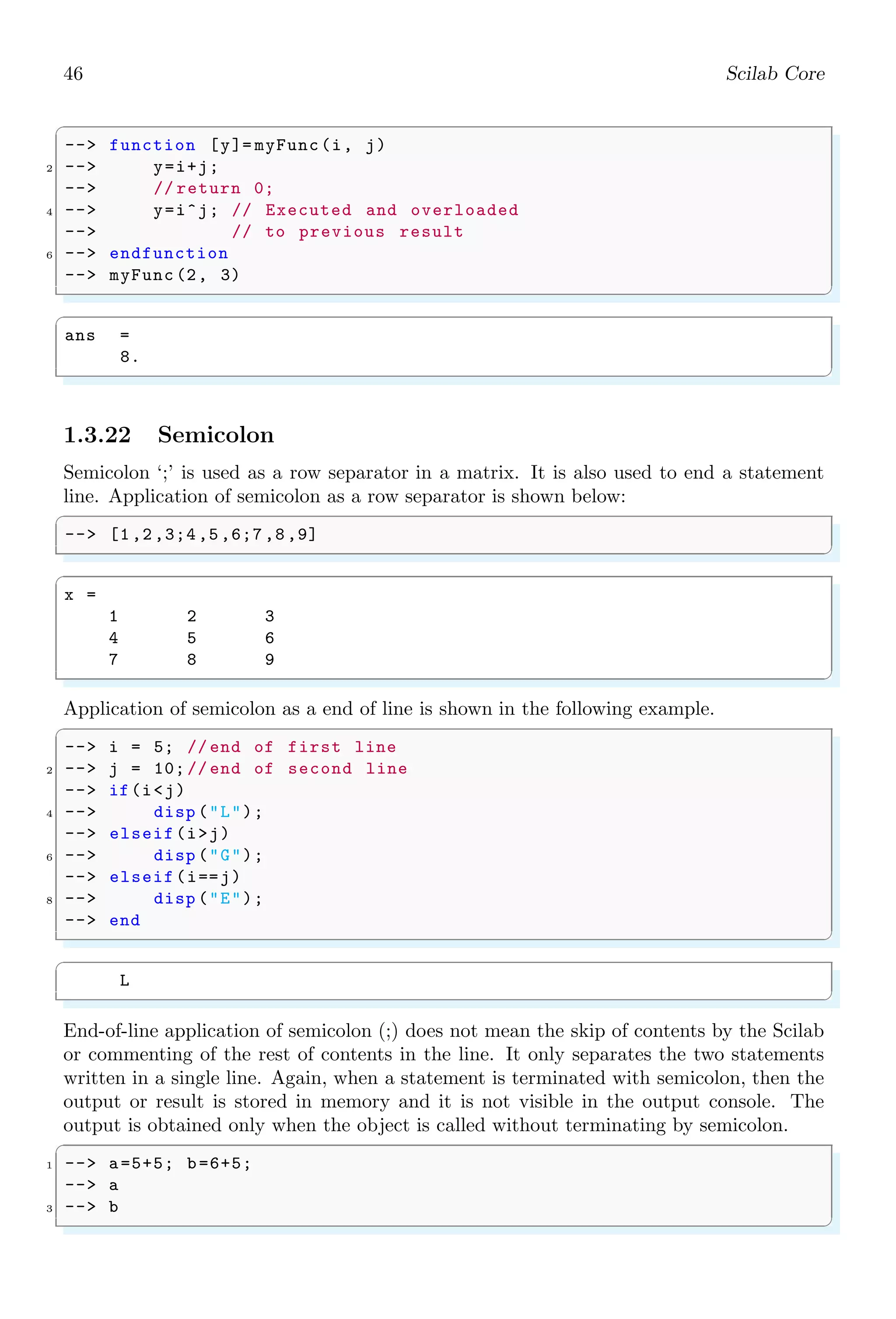
It is also used to return a value from inside of a function. A function is terminated in
execution, when keyword return is encountered.
✞
-- function [y]= myFunc(i, j)
2 -- y=i+j;
-- return 0;
4 -- y=i^j; // Not executed
-- endfunction
6 -- myFunc (2, 3)
✌
✆
✞
ans =
5.
✌
✆](https://image.slidesharecdn.com/scilabhelpbook1of2-220117060625/75/Scilab-help-book-1-of-2-79-2048.jpg)
![46 Scilab Core
✞
-- function [y]= myFunc(i, j)
2 -- y=i+j;
-- // return 0;
4 -- y=i^j; // Executed and overloaded
-- // to previous result
6 -- endfunction
-- myFunc (2, 3)
✌
✆
✞
ans =
8.
✌
✆
1.3.22 Semicolon
Semicolon ‘;’ is used as a row separator in a matrix. It is also used to end a statement
line. Application of semicolon as a row separator is shown below:
✞
-- [1,2,3;4,5,6;7,8,9]
✌
✆
✞
x =
1 2 3
4 5 6
7 8 9
✌
✆
Application of semicolon as a end of line is shown in the following example.
✞
-- i = 5; // end of first line
2 -- j = 10; // end of second line
-- if(ij)
4 -- disp (L);
-- elseif(ij)
6 -- disp (G);
-- elseif(i==j)
8 -- disp (E);
-- end
✌
✆
✞
L
✌
✆
End-of-line application of semicolon (;) does not mean the skip of contents by the Scilab
or commenting of the rest of contents in the line. It only separates the two statements
written in a single line. Again, when a statement is terminated with semicolon, then the
output or result is stored in memory and it is not visible in the output console. The
output is obtained only when the object is called without terminating by semicolon.
✞
1 -- a=5+5; b=6+5;
-- a
3 -- b
✌
✆](https://image.slidesharecdn.com/scilabhelpbook1of2-220117060625/75/Scilab-help-book-1-of-2-80-2048.jpg)
![1.3. ARITHMETICAL KEYWORDS 47
✞
a =
10.
b =
11.
✌
✆
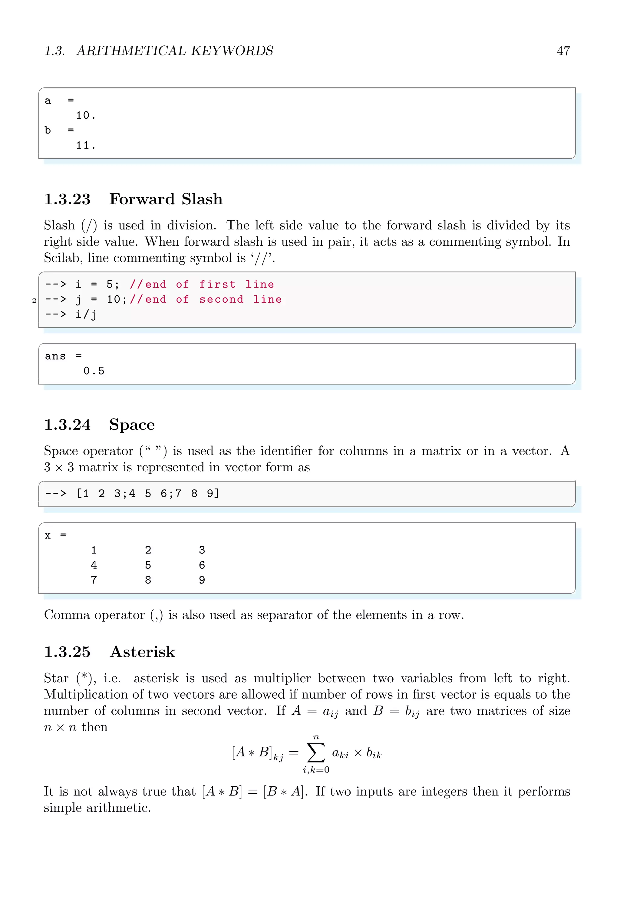
1.3.23 Forward Slash
Slash (/) is used in division. The left side value to the forward slash is divided by its
right side value. When forward slash is used in pair, it acts as a commenting symbol. In
Scilab, line commenting symbol is ‘//’.
✞
-- i = 5; // end of first line
2 -- j = 10; // end of second line
-- i/j
✌
✆
✞
ans =
0.5
✌
✆
1.3.24 Space
Space operator (“ ”) is used as the identifier for columns in a matrix or in a vector. A
3 × 3 matrix is represented in vector form as
✞
-- [1 2 3;4 5 6;7 8 9]
✌
✆
✞
x =
1 2 3
4 5 6
7 8 9
✌
✆
Comma operator (,) is also used as separator of the elements in a row.
1.3.25 Asterisk
Star (*), i.e. asterisk is used as multiplier between two variables from left to right.
Multiplication of two vectors are allowed if number of rows in first vector is equals to the
number of columns in second vector. If A = aij and B = bij are two matrices of size
n × n then
[A ∗ B]kj =
n
X
i,k=0
aki × bik
It is not always true that [A ∗ B] = [B ∗ A]. If two inputs are integers then it performs
simple arithmetic.](https://image.slidesharecdn.com/scilabhelpbook1of2-220117060625/75/Scilab-help-book-1-of-2-81-2048.jpg)
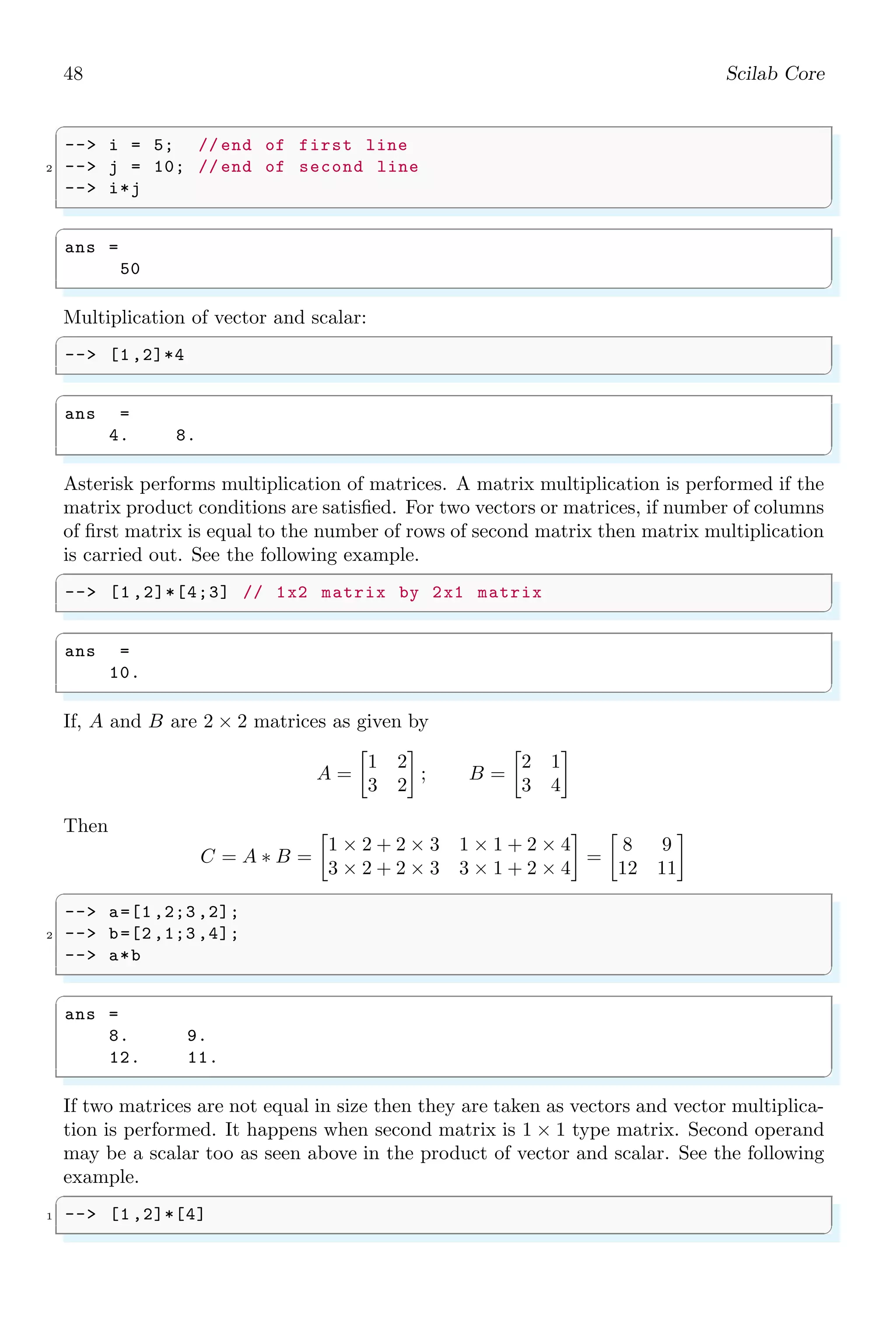
![48 Scilab Core
✞
-- i = 5; // end of first line
2 -- j = 10; // end of second line
-- i*j
✌
✆
✞
ans =
50
✌
✆
Multiplication of vector and scalar:
✞
-- [1 ,2]*4
✌
✆
✞
ans =
4. 8.
✌
✆
Asterisk performs multiplication of matrices. A matrix multiplication is performed if the
matrix product conditions are satisfied. For two vectors or matrices, if number of columns
of first matrix is equal to the number of rows of second matrix then matrix multiplication
is carried out. See the following example.
✞
-- [1 ,2]*[4;3] // 1x2 matrix by 2x1 matrix
✌
✆
✞
ans =
10.
✌
✆
If, A and B are 2 × 2 matrices as given by
A =
1 2
3 2
; B =
2 1
3 4
Then
C = A ∗ B =
1 × 2 + 2 × 3 1 × 1 + 2 × 4
3 × 2 + 2 × 3 3 × 1 + 2 × 4
=
8 9
12 11
✞
-- a=[1 ,2;3 ,2];
2 -- b=[2 ,1;3 ,4];
-- a*b
✌
✆
✞
ans =
8. 9.
12. 11.
✌
✆
If two matrices are not equal in size then they are taken as vectors and vector multiplica-
tion is performed. It happens when second matrix is 1 × 1 type matrix. Second operand
may be a scalar too as seen above in the product of vector and scalar. See the following
example.
✞
1 -- [1 ,2]*[4]
✌
✆](https://image.slidesharecdn.com/scilabhelpbook1of2-220117060625/75/Scilab-help-book-1-of-2-82-2048.jpg)
![1.4. CORE KEYWORDS 49
✞
ans =
4. 8.
✌
✆
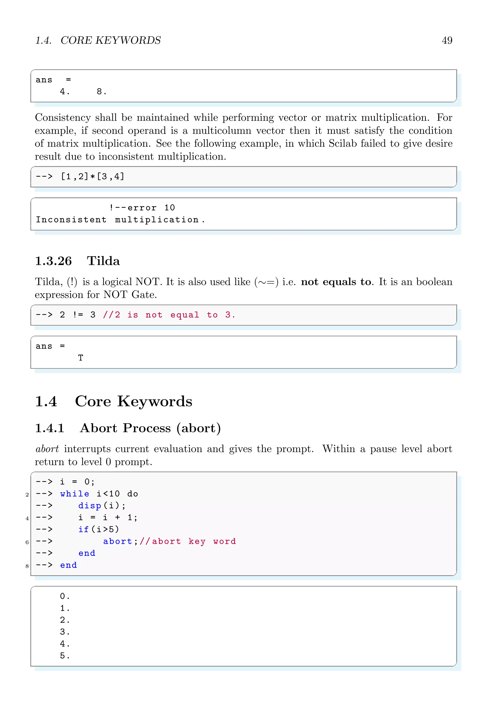
Consistency shall be maintained while performing vector or matrix multiplication. For
example, if second operand is a multicolumn vector then it must satisfy the condition
of matrix multiplication. See the following example, in which Scilab failed to give desire
result due to inconsistent multiplication.
✞
-- [1 ,2]*[3 ,4]
✌
✆
✞
!--error 10
Inconsistent multiplication .
✌
✆
1.3.26 Tilda
Tilda, (!) is a logical NOT. It is also used like (∼=) i.e. not equals to. It is an boolean
expression for NOT Gate.
✞
-- 2 != 3 //2 is not equal to 3.
✌
✆
✞
ans =
T
✌
✆
1.4 Core Keywords
1.4.1 Abort Process (abort)
abort interrupts current evaluation and gives the prompt. Within a pause level abort
return to level 0 prompt.
✞
-- i = 0;
2 -- while i10 do
-- disp (i);
4 -- i = i + 1;
-- if(i5)
6 -- abort;// abort key word
-- end
8 -- end
✌
✆
✞
0.
1.
2.
3.
4.
5.
✌
✆](https://image.slidesharecdn.com/scilabhelpbook1of2-220117060625/75/Scilab-help-book-1-of-2-83-2048.jpg)
![50 Scilab Core
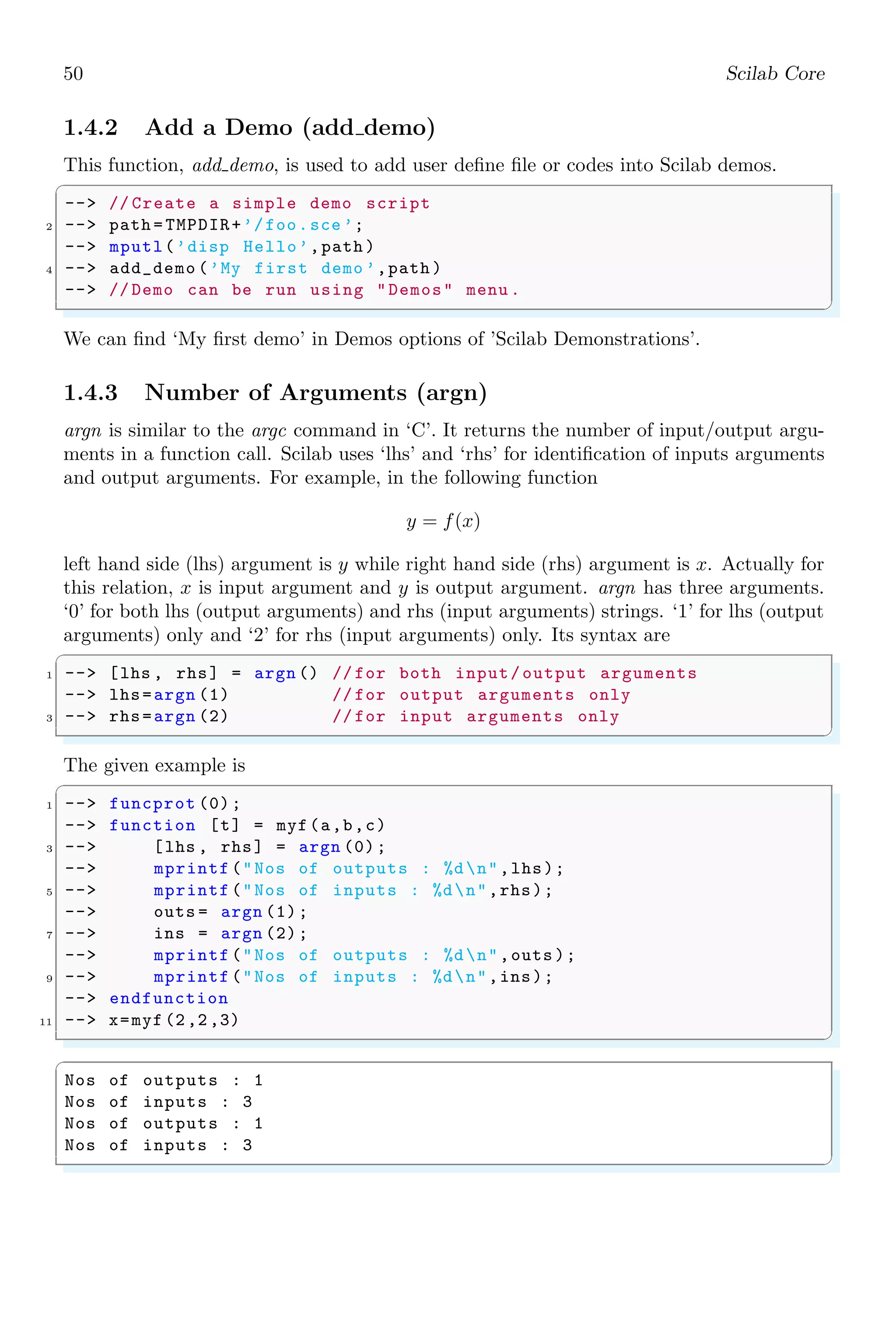
1.4.2 Add a Demo (add demo)
This function, add demo, is used to add user define file or codes into Scilab demos.
✞
-- // Create a simple demo script
2 -- path = TMPDIR+’/foo.sce ’;
-- mputl(’disp Hello’,path )
4 -- add_demo (’My first demo ’,path )
-- // Demo can be run using Demos menu .
✌
✆
We can find ‘My first demo’ in Demos options of ’Scilab Demonstrations’.
1.4.3 Number of Arguments (argn)
argn is similar to the argc command in ‘C’. It returns the number of input/output argu-
ments in a function call. Scilab uses ‘lhs’ and ‘rhs’ for identification of inputs arguments
and output arguments. For example, in the following function
y = f(x)
left hand side (lhs) argument is y while right hand side (rhs) argument is x. Actually for
this relation, x is input argument and y is output argument. argn has three arguments.
‘0’ for both lhs (output arguments) and rhs (input arguments) strings. ‘1’ for lhs (output
arguments) only and ‘2’ for rhs (input arguments) only. Its syntax are
✞
1 -- [lhs , rhs] = argn () // for both input/output arguments
-- lhs=argn (1) // for output arguments only
3 -- rhs=argn (2) // for input arguments only
✌
✆
The given example is
✞
1 -- funcprot (0);
-- function [t] = myf(a,b,c)
3 -- [lhs , rhs] = argn (0);
-- mprintf (Nos of outputs : %dn,lhs);
5 -- mprintf (Nos of inputs : %dn,rhs);
-- outs = argn (1);
7 -- ins = argn (2);
-- mprintf (Nos of outputs : %dn,outs );
9 -- mprintf (Nos of inputs : %dn,ins);
-- endfunction
11 -- x=myf (2,2,3)
✌
✆
✞
Nos of outputs : 1
Nos of inputs : 3
Nos of outputs : 1
Nos of inputs : 3
✌
✆](https://image.slidesharecdn.com/scilabhelpbook1of2-220117060625/75/Scilab-help-book-1-of-2-84-2048.jpg)
![1.4. CORE KEYWORDS 51
1.4.4 Banner
It shows the default banner of Scilab.
✞
-- banner ()
✌
✆
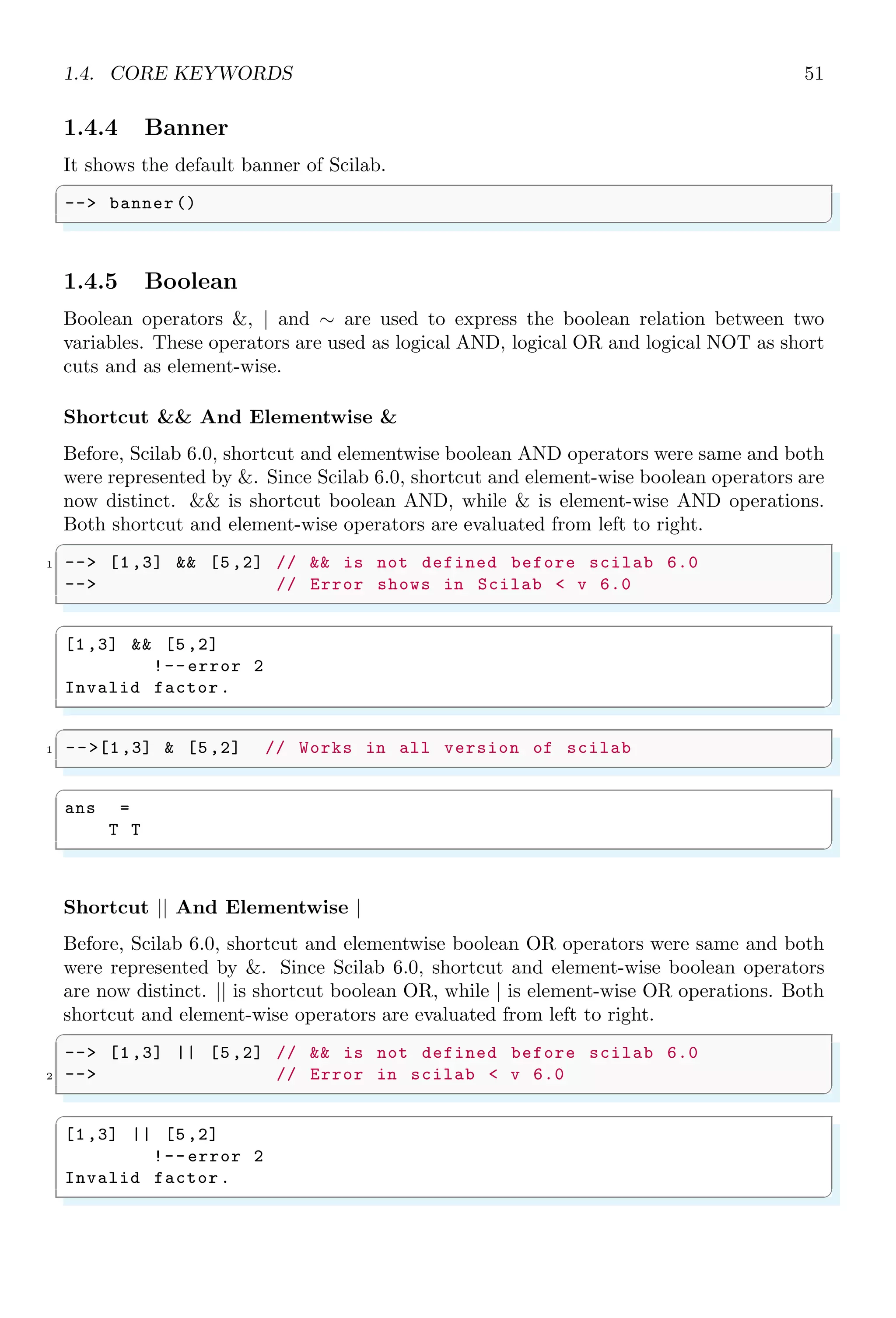
1.4.5 Boolean
Boolean operators , | and ∼ are used to express the boolean relation between two
variables. These operators are used as logical AND, logical OR and logical NOT as short
cuts and as element-wise.
Shortcut And Elementwise
Before, Scilab 6.0, shortcut and elementwise boolean AND operators were same and both
were represented by . Since Scilab 6.0, shortcut and element-wise boolean operators are
now distinct. is shortcut boolean AND, while is element-wise AND operations.
Both shortcut and element-wise operators are evaluated from left to right.
✞
1 -- [1,3] [5,2] // is not defined before scilab 6.0
-- // Error shows in Scilab v 6.0
✌
✆
✞
[1,3] [5,2]
!-- error 2
Invalid factor.
✌
✆
✞
1 --[1,3] [5,2] // Works in all version of scilab
✌
✆
✞
ans =
T T
✌
✆
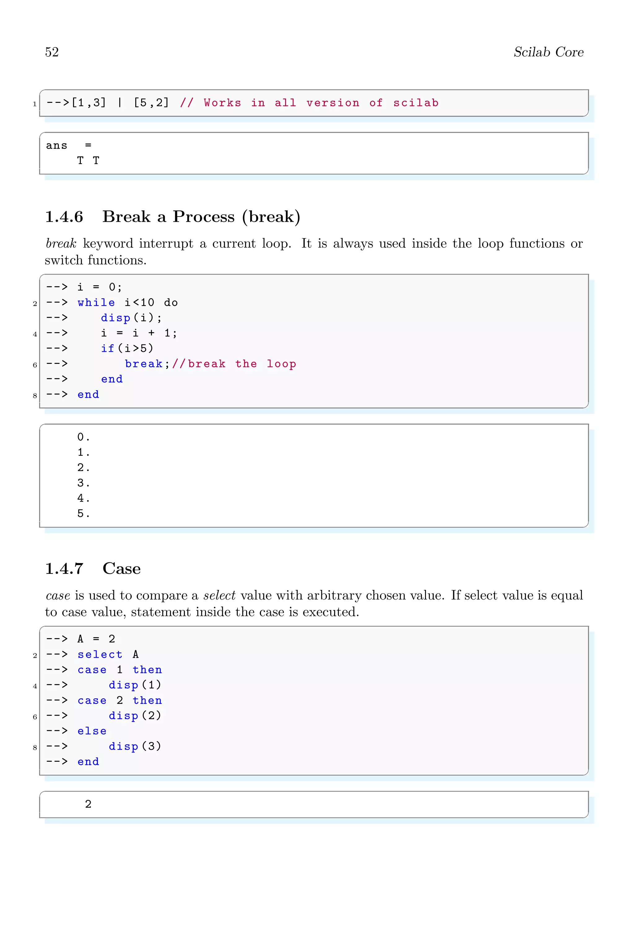
Shortcut || And Elementwise |
Before, Scilab 6.0, shortcut and elementwise boolean OR operators were same and both
were represented by . Since Scilab 6.0, shortcut and element-wise boolean operators
are now distinct. || is shortcut boolean OR, while | is element-wise OR operations. Both
shortcut and element-wise operators are evaluated from left to right.
✞
-- [1,3] || [5,2] // is not defined before scilab 6.0
2 -- // Error in scilab v 6.0
✌
✆
✞
[1,3] || [5,2]
!-- error 2
Invalid factor.
✌
✆](https://image.slidesharecdn.com/scilabhelpbook1of2-220117060625/75/Scilab-help-book-1-of-2-85-2048.jpg)
![52 Scilab Core
✞
1 --[1,3] | [5,2] // Works in all version of scilab
✌
✆
✞
ans =
T T
✌
✆
1.4.6 Break a Process (break)
break keyword interrupt a current loop. It is always used inside the loop functions or
switch functions.
✞
-- i = 0;
2 -- while i10 do
-- disp (i);
4 -- i = i + 1;
-- if(i5)
6 -- break;// break the loop
-- end
8 -- end
✌
✆
✞
0.
1.
2.
3.
4.
5.
✌
✆
1.4.7 Case
case is used to compare a select value with arbitrary chosen value. If select value is equal
to case value, statement inside the case is executed.
✞
-- A = 2
2 -- select A
-- case 1 then
4 -- disp (1)
-- case 2 then
6 -- disp (2)
-- else
8 -- disp (3)
-- end
✌
✆
✞
2
✌
✆](https://image.slidesharecdn.com/scilabhelpbook1of2-220117060625/75/Scilab-help-book-1-of-2-86-2048.jpg)
![1.4. CORE KEYWORDS 59
✞
!--error 10
! This value must be an integer!
✌
✆
An error number as argument is deprecated since Scilab 6.0 onward.
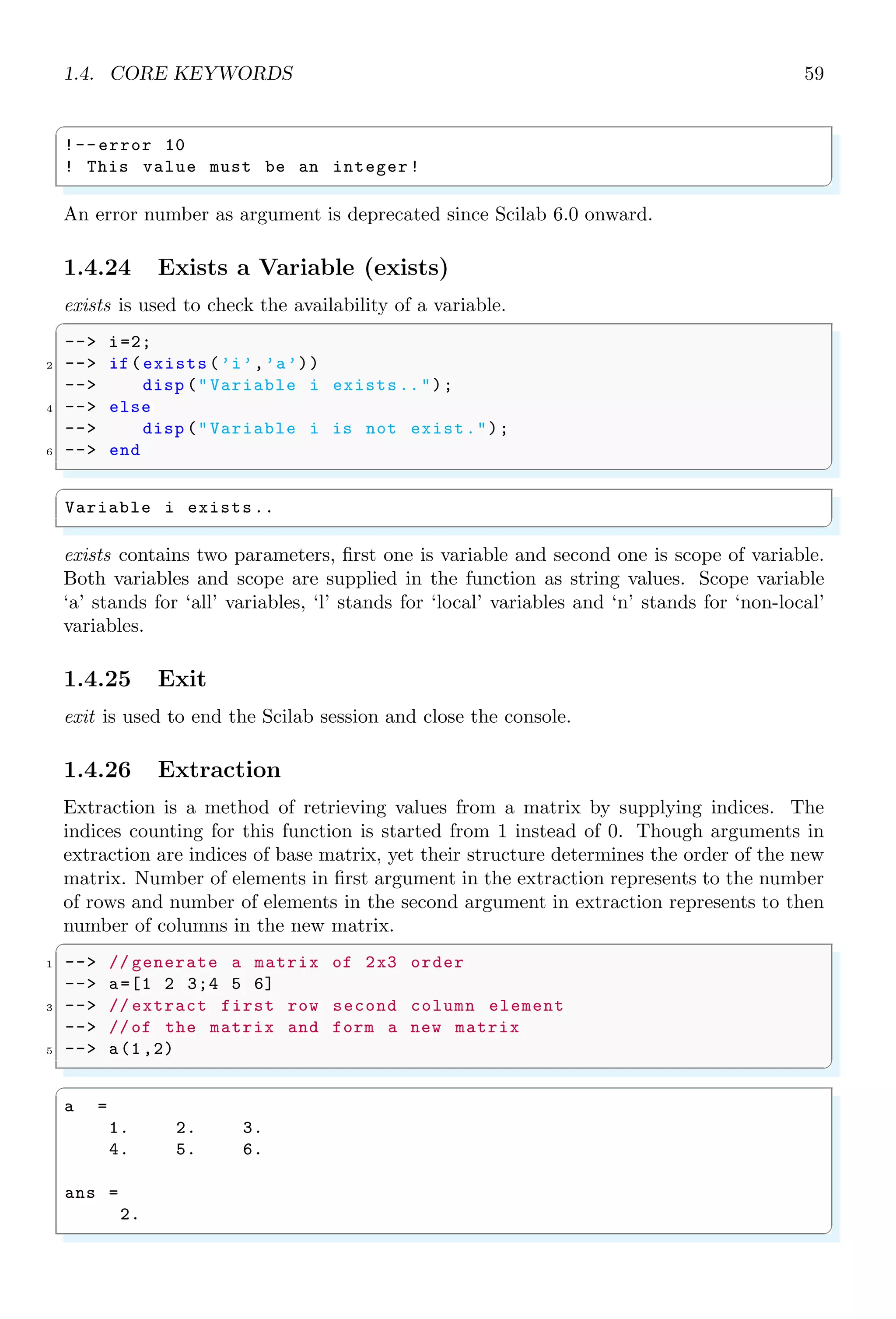
1.4.24 Exists a Variable (exists)
exists is used to check the availability of a variable.
✞
-- i=2;
2 -- if(exists(’i’,’a’))
-- disp (Variable i exists..);
4 -- else
-- disp (Variable i is not exist.);
6 -- end
✌
✆
✞
Variable i exists..
✌
✆
exists contains two parameters, first one is variable and second one is scope of variable.
Both variables and scope are supplied in the function as string values. Scope variable
‘a’ stands for ‘all’ variables, ‘l’ stands for ‘local’ variables and ‘n’ stands for ‘non-local’
variables.
1.4.25 Exit
exit is used to end the Scilab session and close the console.
1.4.26 Extraction
Extraction is a method of retrieving values from a matrix by supplying indices. The
indices counting for this function is started from 1 instead of 0. Though arguments in
extraction are indices of base matrix, yet their structure determines the order of the new
matrix. Number of elements in first argument in the extraction represents to the number
of rows and number of elements in the second argument in extraction represents to then
number of columns in the new matrix.
✞
1 -- // generate a matrix of 2x3 order
-- a=[1 2 3;4 5 6]
3 -- // extract first row second column element
-- //of the matrix and form a new matrix
5 -- a(1,2)
✌
✆
✞
a =
1. 2. 3.
4. 5. 6.
ans =
2.
✌
✆](https://image.slidesharecdn.com/scilabhelpbook1of2-220117060625/75/Scilab-help-book-1-of-2-93-2048.jpg)
![60 Scilab Core
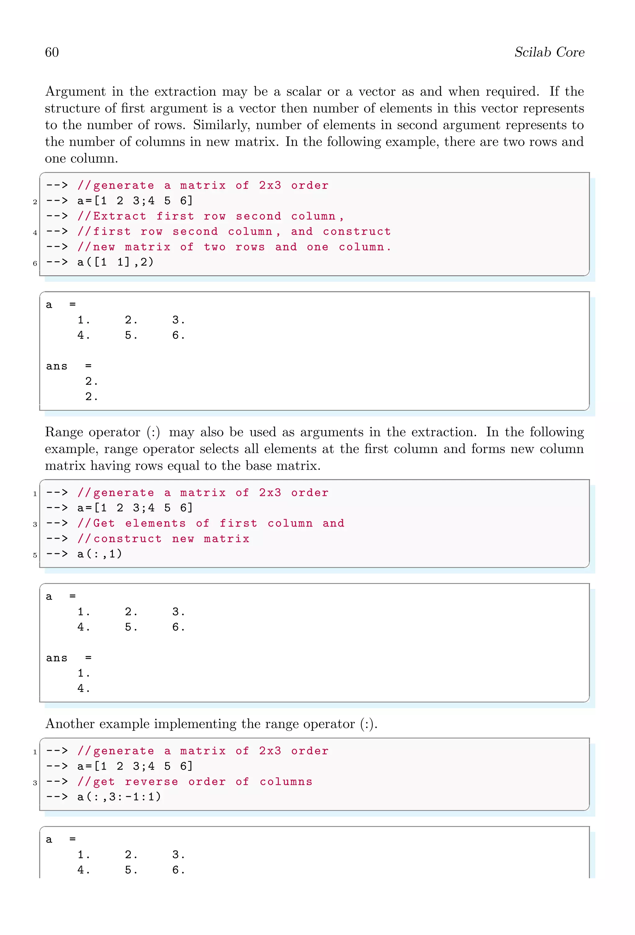
Argument in the extraction may be a scalar or a vector as and when required. If the
structure of first argument is a vector then number of elements in this vector represents
to the number of rows. Similarly, number of elements in second argument represents to
the number of columns in new matrix. In the following example, there are two rows and
one column.
✞
-- // generate a matrix of 2x3 order
2 -- a=[1 2 3;4 5 6]
-- // Extract first row second column ,
4 -- // first row second column , and construct
-- // new matrix of two rows and one column.
6 -- a([1 1],2)
✌
✆
✞
a =
1. 2. 3.
4. 5. 6.
ans =
2.
2.
✌
✆
Range operator (:) may also be used as arguments in the extraction. In the following
example, range operator selects all elements at the first column and forms new column
matrix having rows equal to the base matrix.
✞
1 -- // generate a matrix of 2x3 order
-- a=[1 2 3;4 5 6]
3 -- // Get elements of first column and
-- // construct new matrix
5 -- a(:,1)
✌
✆
✞
a =
1. 2. 3.
4. 5. 6.
ans =
1.
4.
✌
✆
Another example implementing the range operator (:).
✞
1 -- // generate a matrix of 2x3 order
-- a=[1 2 3;4 5 6]
3 -- // get reverse order of columns
-- a(: ,3: -1:1)
✌
✆
✞
a =
1. 2. 3.
4. 5. 6.](https://image.slidesharecdn.com/scilabhelpbook1of2-220117060625/75/Scilab-help-book-1-of-2-94-2048.jpg)
![62 Scilab Core
✞
0.2164633 0.8833888
✌
✆
In exponential format
✞
1 -- x=rand (1,2); // Two random numbers
-- format(’e’ ,10);
3 -- x
✌
✆
✞
6.525D-01 3.076D -01
✌
✆
If you change the format of numbers into exponential then after finishing the calculations,
reset the format of numbers into variable format.
1.4.29 MD5 Hash (getmd5)
getmd5 returns the md5 checksum value of a string or file name.
✞
1 -- getmd5 ([’hello’ ; ’world’],’string ’)
✌
✆
✞
ans =
!5d41402 abc4b2a76b9719 d911017c592 !
!7d793037a0760186574 b0282 f2f435e7 !
✌
✆
For a file name
✞
1 -- getmd5( SCI+’/modules /core /etc/’+[’core .start’ ’core .quit ’])
✌
✆
✞
ans =
! ac68ad2e1905 ed5ec 12331ab91a25864
aba88d66950049 bd 1130 a7d9674 dc5a8 !
✌
✆
1.4.30 Get Memory
getmemory returns free and total system memory.
✞
1 -- [free , total]= getmemory ()
✌
✆
✞
total =
2.066D+06
free =
1.167D+06
✌
✆](https://image.slidesharecdn.com/scilabhelpbook1of2-220117060625/75/Scilab-help-book-1-of-2-96-2048.jpg)
![1.4. CORE KEYWORDS 63
1.4.31 Get Modules
getmodules returns list of modules installed in Scilab.
✞
-- res=getmodules ()
✌
✆
1.4.32 Get Operating System
getos returns Operating System name and version.
✞
1 -- [OS , version] = getos()
✌
✆
✞
version =
XP
OS =
Windows
✌
✆
1.4.33 Get Scilab Mode
getscilabmode returns the mode of Scilab.
✞
-- getscilabmode ()
✌
✆
✞
ans =
STD
✌
✆
1.4.34 Get Shell
getshell returns current command interpreter.
✞
-- getshell ()
✌
✆
✞
ans =
cmd
✌
✆
1.4.35 Get Variale Stack
getvariablesonstack returns variable names on stack of Scilab.
✞
-- getvariablesonstack ();
2 -- getvariablesonstack (’local’);
-- getvariablesonstack (’global’);
✌
✆](https://image.slidesharecdn.com/scilabhelpbook1of2-220117060625/75/Scilab-help-book-1-of-2-97-2048.jpg)
![64 Scilab Core
1.4.36 Version
getversion returns scilab and modules version information.
✞
1 -- version = getversion (’Scilab’)
✌
✆
✞
version =
5.000D+00 4.000D+00 0.000D+00 1.349D+09
✌
✆
1.4.37 Insertion
It is a process of adding an element in a matrix. It is reverse process of Extraction. Let
a matrix ‘a’ of order 2 × 3
✞
-- a=[1 2 3;4 5 6]
✌
✆
✞
a =
1. 2. 3.
4. 5. 6.
✌
✆
We can add an element ‘10’ at (1,1) position by indexing the element and assigning value
to that index of the array.
✞
1 -- a(1,2)=10
✌
✆
✞
a =
1. 10. 3.
4. 5. 6.
✌
✆
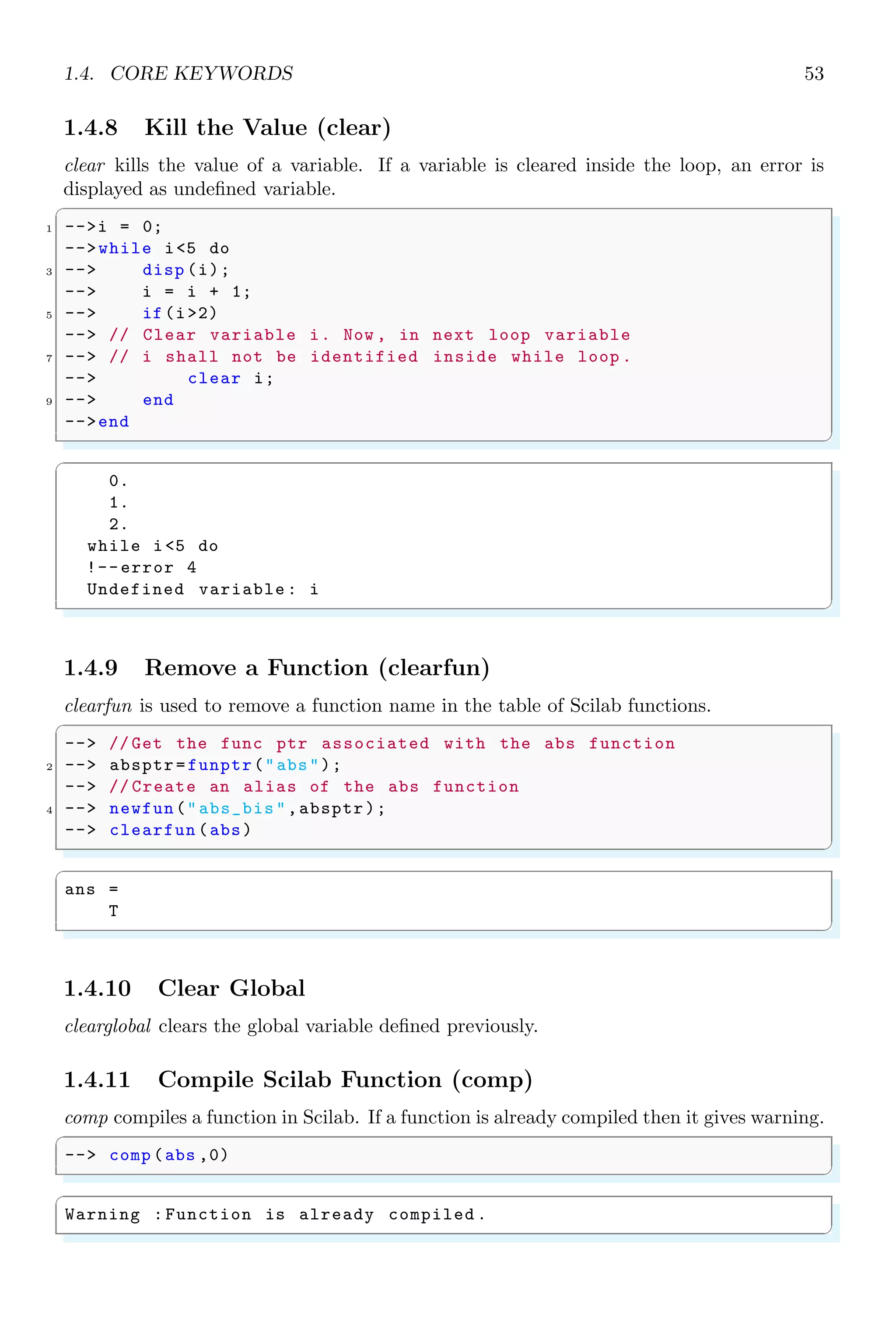
It is a keyword that executes a statement conditionally.
✞
1 -- i = 5;
-- j = 10;
3 -- if(i==j)//If both i j are equal
-- disp (E);// print ’E’ in output console.
5 -- elseif(ij)
-- disp (N);
7 -- end
✌
✆
✞
N
✌
✆
Each if started should be closed by using end command](https://image.slidesharecdn.com/scilabhelpbook1of2-220117060625/75/Scilab-help-book-1-of-2-98-2048.jpg)
![1.4. CORE KEYWORDS 65
1.4.38 Interface Properties (intppty)
intppty sets interface argument passing properties.
✞
1 -- funs = intppty ()
✌
✆
✞
funs =
6. 13. 16. 19. 21. 23. 41. 42. 71.
✌
✆
1.4.39 Inverse Coefficients (inv coeff)
inv coeff is used to build a polynomial matrix by using coefficients.
✞
-- A=int (10* rand (2,6));
2 -- P=inv_coeff (A,1)// second argument is the
-- // order of polynomial .
✌
✆
✞
P =
8 + 3x 3 + 7x 9 + 4x
5 + 3x 3 + 2x 9 + 2x
✌
✆
The same coefficients are used for second order polynomial matrix.
✞
1 -- A=int (10* rand (2,6));
-- P=inv_coeff (A,2)// second argument is the
3 -- // order of polynomial .
✌
✆
P =
2 + 6x + 8x2
8x + 5x2
7 + 6x 3 + 6x + 6x2
1.4.40 Is Error
iserror returns ‘true’ or ‘false’ if there is error or not. This function is removed since
Scilab 6.
✞
1 -- iserror ([n])
✌
✆
If ‘n 0’, all errors are tested other wise only error numbered ‘n’ is tested.](https://image.slidesharecdn.com/scilabhelpbook1of2-220117060625/75/Scilab-help-book-1-of-2-99-2048.jpg)
![1.4. CORE KEYWORDS 67
1.4.43 Last Error (lasterror)
lasterror returns the number of error occurs recently.
✞
-- ierr = execstr(’a=zzzzzzz ’,’errcatch ’);
2 -- if ierr 0 then
-- disp (lasterror ())
4 -- end
✌
✆
✞
Undefined variable : zzzzzzz
✌
✆
1.4.44 Macro To List
macr2lst primitive converts a compiled Scilab function name into a list which codes the
internal representation of the function (Reverse Polish Notation). This function will not
available since Scilab 6 and above.
✞
1 -- function y=myF(x, flag )
-- if flag then
3 -- y=sin(x)
-- else
5 -- y=cos(x)
-- end
7 -- endfunction
-- L=macr2lst (myF)
9 -- fun2string (L) // This function is removed in scilab 6.0
✌
✆
✞
ans =
!function y=myF(x,flag ) !
! if flag then !
! y = sin(x) !
! else !
! y = cos(x) !
! end , !
!endfunction !
✌
✆
1.4.45 Macro To Tree
macro2tree primitive converts a compiled Scilab function name into a tree.
✞
-- tree = macr2tree (cosh );
2 -- txt=tree2code (tree ,%T);
-- write(%io (2),txt ,’(a)’);
✌
✆
✞
function [t] = cosh (z)
//
// PURPOSE](https://image.slidesharecdn.com/scilabhelpbook1of2-220117060625/75/Scilab-help-book-1-of-2-101-2048.jpg)
![68 Scilab Core
// element wise hyperbolic cosine
//
// METHOD
// 1/ in the real case use
//
// cosh (z) = 0.5 (exp(|z|) + exp(-|z|))
// = 0.5 ( y + 1/y ) with y = exp(|z|)
//
// The absolute value avoids the problem of a
// division by zero arising with the formula
// cosh (z) = 0.5 ( y + 1/y ), y=exp(z)
// when ieee = 0 for z such that exp(z) equal 0 in
// floating point arithmetic (approximately z -745)
//
// 2/ in the complex case use : cosh (z) = cos(i z)
//
rhs = argn (2);
if rhs$ sim $=1 then
error(msprintf (gettext (%s: Wrong number of input ..
argument (s): %d expected .n) ,cosh ,1));
end;
if type (z)$ sim $=1 then
error(msprintf (gettext (%s: Wrong type for input ..
argument #%d: Real or complex ..
matrix expected .n) ,cosh ,1));
end;
if isreal(z) then
y = exp(abs(z));
t = 0.5*(y+1 ./y)
else
t = cos(imult(z))
end;
endfunction
✌
✆
1.4.46 Matrices
Matrices are the arrangement of integers or variables into rows and columns. These
integers and variables are called elements of the vector of matrix.
✞
-- A=[1 ,2 ,3;4 ,5 ,6]
✌
✆
✞
A =
1. 2. 3.
4. 5. 6.
✌
✆
1.4.47 Matrix
matrix function is used to arrange elements in desired format of rows and columns. This
function is useful in rearranging of elements in desired order of matrix. matrix arranges](https://image.slidesharecdn.com/scilabhelpbook1of2-220117060625/75/Scilab-help-book-1-of-2-102-2048.jpg)
![74 Scilab Core
✞
1 --r=rand (10,1, uniform ) //10 rows 1 columns
✌
✆
✞
r =
0.7560439
0.0002211
0.3303271
0.6653811
0.6283918
0.8497452
0.6857310
0.8782165
0.0683740
0.5608486
✌
✆
1.4.58 Read Gateway
Each module is assigned a gateway id and this id can be assessed by using readgateway
command.
✞
1 -- [primitives ,primitivesID ,gatewayID ] = readgateway (’core ’);
-- primitives (1); // ’debug ’ primitive
3 -- primitivesID (1); // 1 is ID of ’debug ’ in ’core ’ gateway
-- gatewayID (1) // 13 is ID of ’core ’ gateway in Scilab
✌
✆
✞
ans =
13
✌
✆
1.4.59 Resume
resume invokes Scilab to return to the current execution or resume the current execution
and copy some local variables. Scilab asks for resume or abort keywords when a loop is
paused by pause command. If resume is entered, then loop is started again and if abort is
entered then loop is exits. pause, resume and abort are treated as inter process interrupts.
✞
-- i = 0;
2 -- while i10 do
-- disp (i);
4 -- i = i + 1;
-- if(i5)
6 -- pause; // pause the loop
-- end
8 -- end
✌
✆
✞
0.
1.
2.](https://image.slidesharecdn.com/scilabhelpbook1of2-220117060625/75/Scilab-help-book-1-of-2-108-2048.jpg)
![76 Scilab Core
1.4.63 Temporary Directory (TMPDIR)
‘TMPDIR’ is a token that points to the path of the temporary directory being used by
Scilab as its scratch directory, or it is being used for storing temprary data, files etc. For
my windows system the Scilab temporary directory path is
✞
1 -- path = TMPDIR;
-- disp (path )
✌
✆
✞
C: DOCUME ~1 ADMINI ~1 LOCALS ~1 Temp SCI_TMP _3104_
✌
✆
1.4.64 Test Matrix
testmatrix is used to generate special matrices, like Magic, Frank and Hilbert matrices.
The type of matrix being generated is identified by the first argument of this function.
For magic matrix, keyword is ‘magi’, for Frank matrix, keyword is ‘frk’ and for Hilbert
matrix, keyword is ‘hilb’. See the following examples, for magic matrix.
✞
1 -- [y]= testmatrix (’magi ’ ,2)
✌
✆
✞
[]
✌
✆
Frank matrix can be generated by
✞
1 -- [y]= testmatrix (’frk ’ ,2)
✌
✆
✞
y =
2. 1.
1. 1.
✌
✆
Hilbert matrix by
✞
1 -- [y]= testmatrix (’hilb ’ ,2)
✌
✆
✞
y =
4. - 6.
- 6. 12.
✌
✆
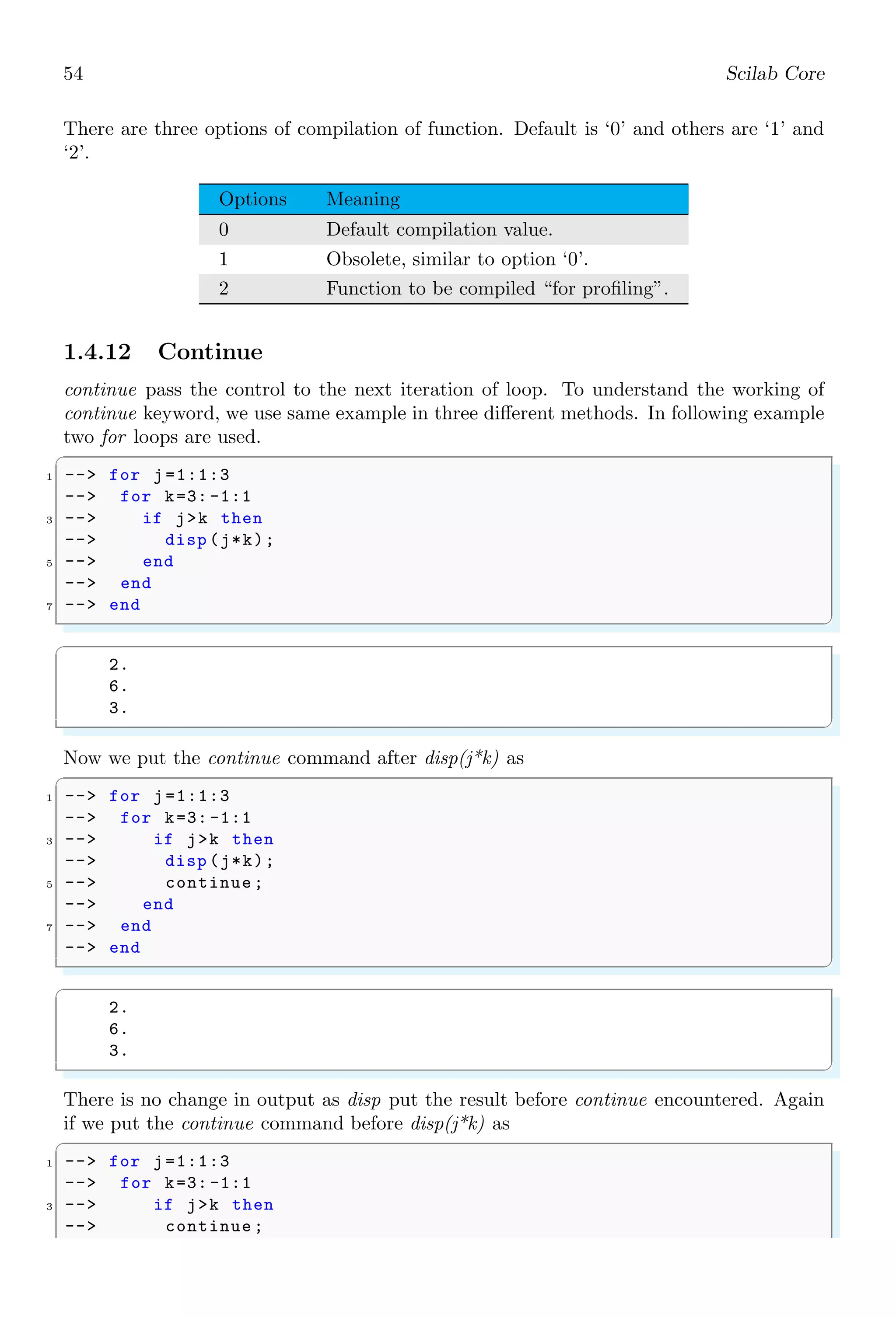
1.4.65 Then
then keyword is used along-with if keyword in the sequence of if-then-else structure. If if
condition is ‘true’ then statement inside the then block are executed otherwise statement
in else block are executed.](https://image.slidesharecdn.com/scilabhelpbook1of2-220117060625/75/Scilab-help-book-1-of-2-110-2048.jpg)
![78 Scilab Core
Code Variable Type
1 sci matrix: a matrix of doubles
2 sci poly: a polynomials matrix
4 sci boolean: a boolean matrix
5 sci sparse: a sparse matrix
6 sci boolean sparse: a sparse boolean matrix
7 sci matlab sparse: a sparse matlab matrix
8 sci ints: a matrix of integers
9 sci handles: a graphical handle
10 sci strings: a matrix of strings
11 sci u function: an uncompiled Scilab function
13 sci c function: a compiled Scilab function
14 sci lib: a library of Scilab functions
15 sci list: a Scilab list
16 sci tlist: a Scilab tlist
17 sci mlist: a Scilab mlist
18 sci struct: a Scilab struct
19 sci cell: a Scilab cell
128 sci pointer : a pointer
✞
1 -- x = 2;
-- [i]= type (x)
✌
✆
✞
i =
1
✌
✆
1.4.68 Integer Data Type
Scilab supports, 8, 16, 32 and 64 signed and unsigned integer data type. Each integer
data type is defined as function
✞
-- int size (input )
2 -- uint size (input )
✌
✆
Where, ‘size’ is any value from 8, 16, 32 and 64. We can convert an integer into any type
among the defined size.
✞
-- int8 ([10 ,12 ,500 ,4000])
2 -- uint8 ([10 ,12 ,500 ,4000])
✌
✆](https://image.slidesharecdn.com/scilabhelpbook1of2-220117060625/75/Scilab-help-book-1-of-2-112-2048.jpg)
![1.4. CORE KEYWORDS 79
✞
ans =
10 12 -12 -96
ans =
10 12 244 160
✌
✆
Other method is by application of function iconvert as
✞
-- iconvert (input , type )
✌
✆
Here, type is any code of the following table.
Type Function Range
0 (reals)
1 int8 [-128, 127]
2 int16 [-32768, 32767]
4 int32 [-2147483648, 2147483647]
8 int64 [-9223372036854775808, 9223372036854775807]
11 uint8 [0, 255]
12 uint16 [0, 65535]
14 uint32 [0, 4294967295]
18 uint64 [0, 18446744073709551615]
During the data conversion, values stored in the memory are not altered. Only method
and length of reading of memory bytes manipulated. For example, an integer is stored in
the memory as shown below. The shown data in each byte is in binary form.
iPtr
11000111 11010111 11001111 11100111
The decimal value of integer is 335280944710. For integer data type, all four bytes are
converted from binary value into decimal value at once. If this integer is converted into
8 bits data type (char type), then data from last byte having binary data 111001112 is
taken and converted. In the above case, output is −25 signed and 231 unsigned.
1.4.69 Varn (varn)
varn returns a polynomial matrix with same coefficients as x but with ‘s’ as symbolic
variable.
✞
1 -- s=poly (0,’s’);
-- p=[s^2+1,s];
3 -- varn (p);
-- varn (p,’x’)
✌
✆](https://image.slidesharecdn.com/scilabhelpbook1of2-220117060625/75/Scilab-help-book-1-of-2-113-2048.jpg)
![1.5. FUNCTIONS 81
✞
-- i = 0
2 -- while i5 do
-- disp (i);
4 -- i = i + 1;
-- end
✌
✆
✞
ans =
0
1
2
3
4
✌
✆
1.5 Functions
Function, in computer science is a set of instructions. This set of instruction is collectively
called a script or code. Codes inside the function are not executed until unless function
is not called. Some times more than one functions or commands are successively used
for a specific purpose. The re-usability of these sets of functions or commands is very
problematic. Hence these set of functions or commands are put inside a new function
defined by user. Now this new defined function can be used as and when required
1.5.1 Defining Own Function
In Scilab, user can define their own functions. The syntax is
✞
-- // begin of function
2 -- function [outputs ]= myF(argumets )
-- /* Function Statements */
4 -- endfunction
-- // end the function
✌
✆
Any number of input arguments and output variables may be used in a function. Each
input and output variable shall be separated by a comma. Scilab function is initialize
by using the function keyword. This keyword is followed by output variables, either in
vector form or in matrix form, to which result is assigned by the function. Then, ‘=’
sign is followed by the valid name of function with or without function parameters. Each
function that is initiated should be terminated by using keyword endfunction keyword.
See the following example:
✞
1 -- // begin of function
-- function [x, y]= myF(a, b)
3 -- x=a+b // expressions
-- y=a-b // expressions
5 -- endfunction
-- // end the function
✌
✆](https://image.slidesharecdn.com/scilabhelpbook1of2-220117060625/75/Scilab-help-book-1-of-2-115-2048.jpg)
![82 Scilab Core
When function is called like
✞
-- [x,y]= myF (5,2);
✌
✆
output on the screen is visible like
✞
x =
7.
y =
3.
✌
✆
If an output variable is not declared inside the function body, either as a returned
value or as a declared value, then when function is called with full decoration, will show
errors.
✞
-- function [x, y]= myF(a, b)
2 -- x=a+b; // expressions
-- endfunction
✌
✆
Since Scilab 6.0 version, a function may also be finished by using only ‘end’ keyword. deff
function may be used for inline definition of a function. Its syntax is
✞
1 -- deff (’[out var ]= func name (var 1, var 2)’ ,..
’function statements ’)
✌
✆
To define function z = x + y as inline function, method is
✞
-- deff (’[z]=f(x,y)’,’z=x+y’)
✌
✆
Here f is function name that would be called later. Since Scilab 6.0, function without
output argument cannot be called in assignment expression anymore. For example,
✞
1 -- function myFunc(i, j)
-- return i+j;
3 -- endfunction
-- r=myFunc (2, 3)// returns error in Scilab = 6.0
✌
✆
1.5.2 Rewriting Own Function
Scilab allow function rewriting with or without same signature. When new function is
written with same name as the existing function has, then new function hides to the
existing function with same name. Now, new function needs the parameter to be passed
to it in accordance with new signature of the function.
✞
-- function myF(a, b)// User defined function .
2 -- z=a+b;
-- disp (z);
4 -- endfunction
-- function myF(a, b)// rewritten function .
6 -- z=a*b;](https://image.slidesharecdn.com/scilabhelpbook1of2-220117060625/75/Scilab-help-book-1-of-2-116-2048.jpg)
![2.1. LINEAR ALGEBRA 87
2Linear Algebra
2.1 Linear Algebra
Linear algebra is the branch of mathematics motivated by a system of linear equations
containing several unknowns.
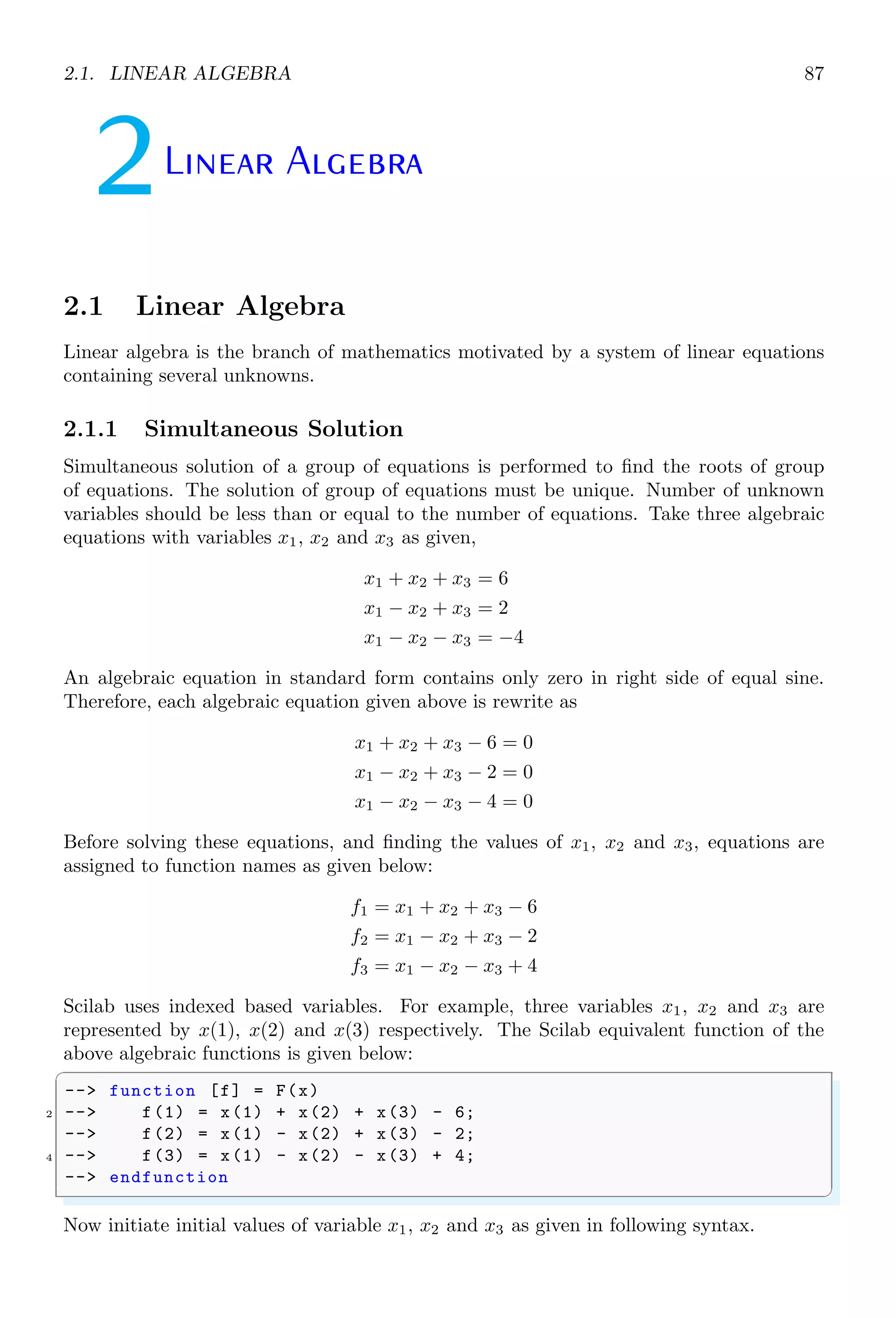
2.1.1 Simultaneous Solution
Simultaneous solution of a group of equations is performed to find the roots of group
of equations. The solution of group of equations must be unique. Number of unknown
variables should be less than or equal to the number of equations. Take three algebraic
equations with variables x1, x2 and x3 as given,
x1 + x2 + x3 = 6
x1 − x2 + x3 = 2
x1 − x2 − x3 = −4
An algebraic equation in standard form contains only zero in right side of equal sine.
Therefore, each algebraic equation given above is rewrite as
x1 + x2 + x3 − 6 = 0
x1 − x2 + x3 − 2 = 0
x1 − x2 − x3 − 4 = 0
Before solving these equations, and finding the values of x1, x2 and x3, equations are
assigned to function names as given below:
f1 = x1 + x2 + x3 − 6
f2 = x1 − x2 + x3 − 2
f3 = x1 − x2 − x3 + 4
Scilab uses indexed based variables. For example, three variables x1, x2 and x3 are
represented by x(1), x(2) and x(3) respectively. The Scilab equivalent function of the
above algebraic functions is given below:
✞
-- function [f] = F(x)
2 -- f(1) = x(1) + x(2) + x(3) - 6;
-- f(2) = x(1) - x(2) + x(3) - 2;
4 -- f(3) = x(1) - x(2) - x(3) + 4;
-- endfunction
✌
✆
Now initiate initial values of variable x1, x2 and x3 as given in following syntax.](https://image.slidesharecdn.com/scilabhelpbook1of2-220117060625/75/Scilab-help-book-1-of-2-121-2048.jpg)
![88 Linear Algebra
✞
1 -- x = [1 1 1];
✌
✆
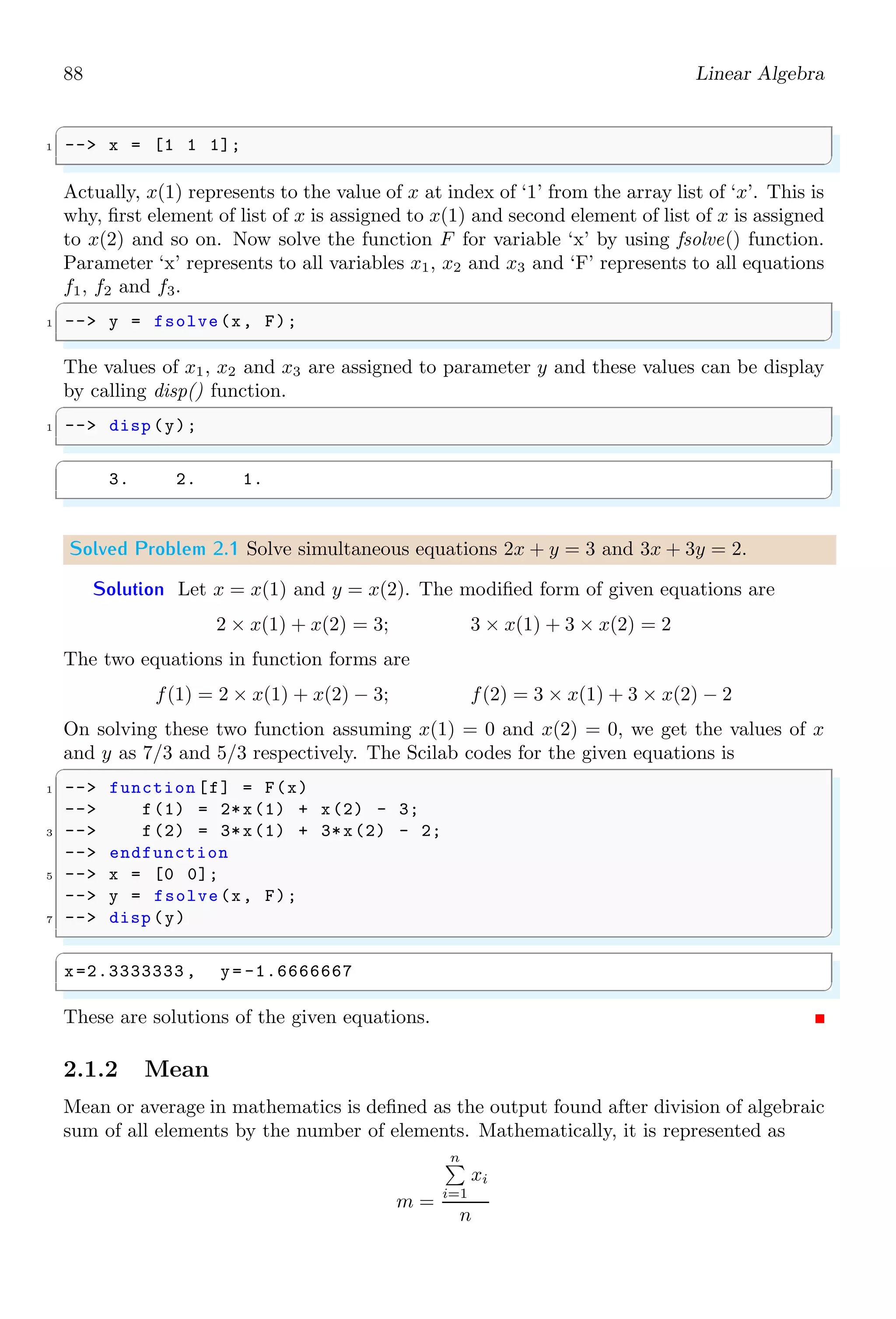
Actually, x(1) represents to the value of x at index of ‘1’ from the array list of ‘x’. This is
why, first element of list of x is assigned to x(1) and second element of list of x is assigned
to x(2) and so on. Now solve the function F for variable ‘x’ by using fsolve() function.
Parameter ‘x’ represents to all variables x1, x2 and x3 and ‘F’ represents to all equations
f1, f2 and f3.
✞
1 -- y = fsolve(x, F);
✌
✆
The values of x1, x2 and x3 are assigned to parameter y and these values can be display
by calling disp() function.
✞
1 -- disp (y);
✌
✆
✞
3. 2. 1.
✌
✆
Solved Problem 2.1 Solve simultaneous equations 2x + y = 3 and 3x + 3y = 2.
Solution Let x = x(1) and y = x(2). The modified form of given equations are
2 × x(1) + x(2) = 3; 3 × x(1) + 3 × x(2) = 2
The two equations in function forms are
f(1) = 2 × x(1) + x(2) − 3; f(2) = 3 × x(1) + 3 × x(2) − 2
On solving these two function assuming x(1) = 0 and x(2) = 0, we get the values of x
and y as 7/3 and 5/3 respectively. The Scilab codes for the given equations is
✞
1 -- function [f] = F(x)
-- f(1) = 2*x(1) + x(2) - 3;
3 -- f(2) = 3*x(1) + 3*x(2) - 2;
-- endfunction
5 -- x = [0 0];
-- y = fsolve(x, F);
7 -- disp (y)
✌
✆
✞
x=2.3333333 , y= -1.6666667
✌
✆
These are solutions of the given equations.
2.1.2 Mean
Mean or average in mathematics is defined as the output found after division of algebraic
sum of all elements by the number of elements. Mathematically, it is represented as
m =
n
P
i=1
xi
n](https://image.slidesharecdn.com/scilabhelpbook1of2-220117060625/75/Scilab-help-book-1-of-2-122-2048.jpg)
![2.1. LINEAR ALGEBRA 89
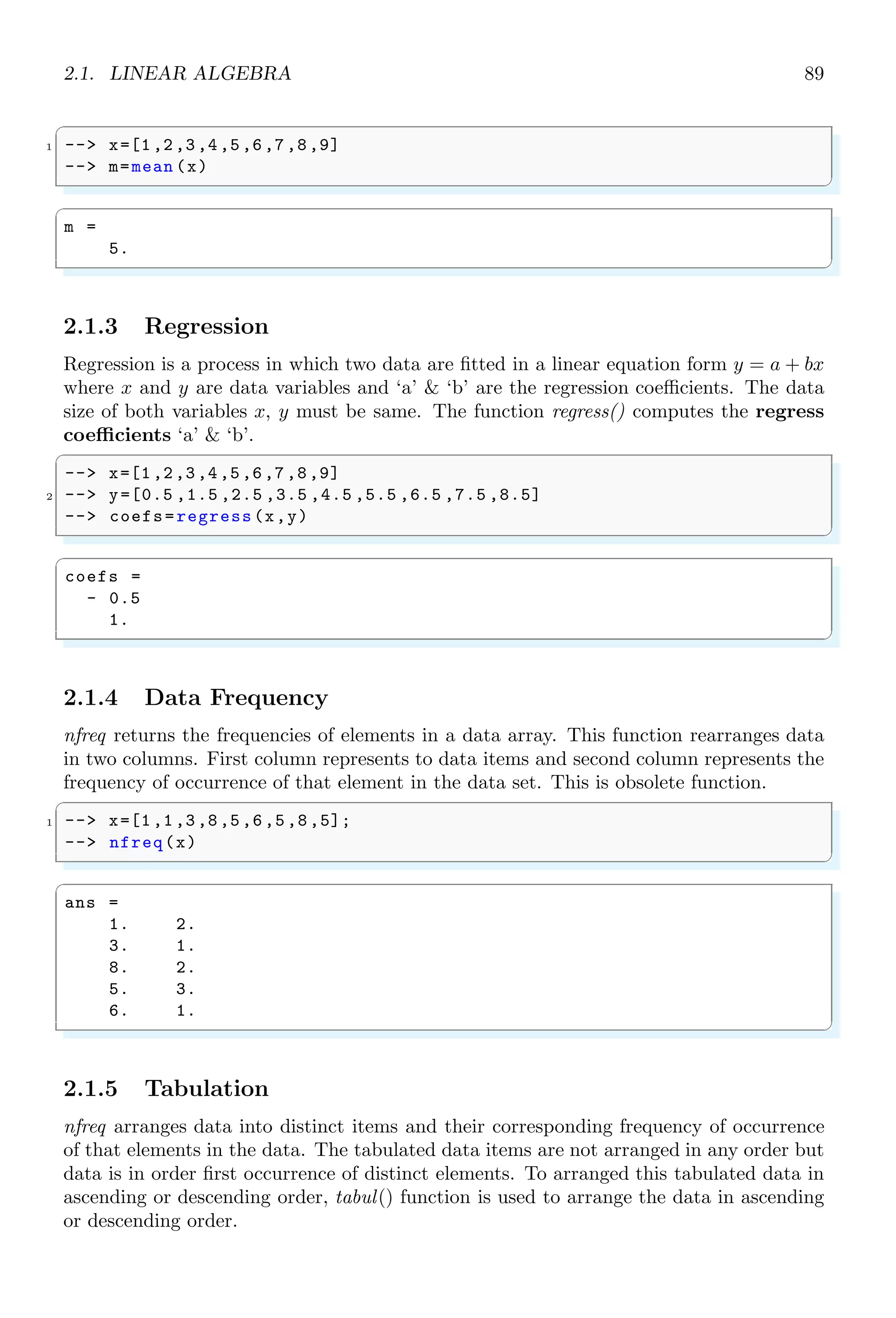
✞
1 -- x=[1,2,3,4,5,6,7,8,9]
-- m=mean (x)
✌
✆
✞
m =
5.
✌
✆
2.1.3 Regression
Regression is a process in which two data are fitted in a linear equation form y = a + bx
where x and y are data variables and ‘a’ ‘b’ are the regression coefficients. The data
size of both variables x, y must be same. The function regress() computes the regress
coefficients ‘a’ ‘b’.
✞
-- x=[1,2,3,4,5,6,7,8,9]
2 -- y=[0.5 ,1.5 ,2.5 ,3.5 ,4.5 ,5.5 ,6.5 ,7.5 ,8.5]
-- coefs=regress(x,y)
✌
✆
✞
coefs =
- 0.5
1.
✌
✆
2.1.4 Data Frequency
nfreq returns the frequencies of elements in a data array. This function rearranges data
in two columns. First column represents to data items and second column represents the
frequency of occurrence of that element in the data set. This is obsolete function.
✞
1 -- x=[1,1,3,8,5,6,5,8,5];
-- nfreq(x)
✌
✆
✞
ans =
1. 2.
3. 1.
8. 2.
5. 3.
6. 1.
✌
✆
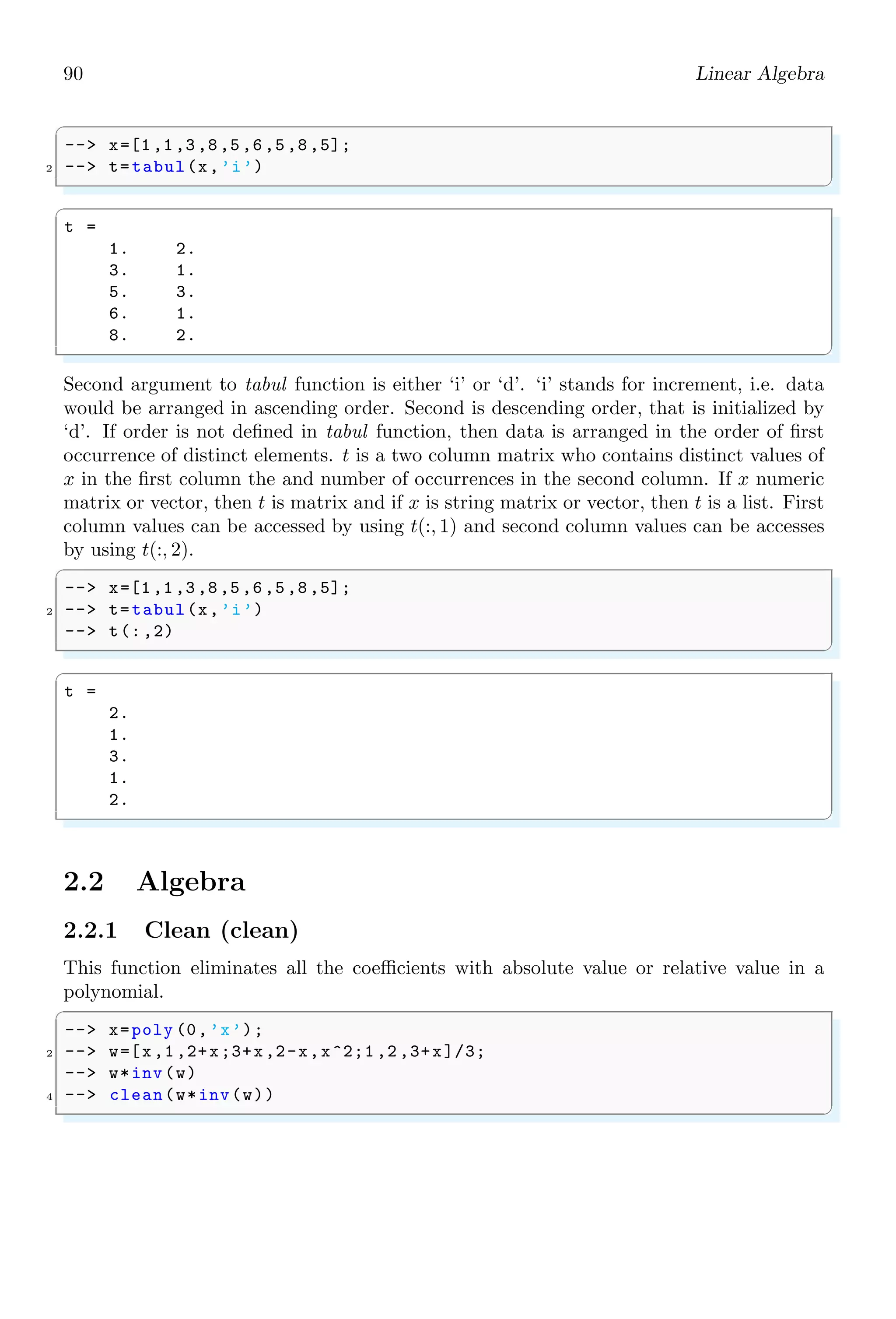
2.1.5 Tabulation
nfreq arranges data into distinct items and their corresponding frequency of occurrence
of that elements in the data. The tabulated data items are not arranged in any order but
data is in order first occurrence of distinct elements. To arranged this tabulated data in
ascending or descending order, tabul() function is used to arrange the data in ascending
or descending order.](https://image.slidesharecdn.com/scilabhelpbook1of2-220117060625/75/Scilab-help-book-1-of-2-123-2048.jpg)
![90 Linear Algebra
✞
-- x=[1,1,3,8,5,6,5,8,5];
2 -- t=tabul(x,’i’)
✌
✆
✞
t =
1. 2.
3. 1.
5. 3.
6. 1.
8. 2.
✌
✆
Second argument to tabul function is either ‘i’ or ‘d’. ‘i’ stands for increment, i.e. data
would be arranged in ascending order. Second is descending order, that is initialized by
‘d’. If order is not defined in tabul function, then data is arranged in the order of first
occurrence of distinct elements. t is a two column matrix who contains distinct values of
x in the first column the and number of occurrences in the second column. If x numeric
matrix or vector, then t is matrix and if x is string matrix or vector, then t is a list. First
column values can be accessed by using t(:, 1) and second column values can be accesses
by using t(:, 2).
✞
-- x=[1,1,3,8,5,6,5,8,5];
2 -- t=tabul(x,’i’)
-- t(:,2)
✌
✆
✞
t =
2.
1.
3.
1.
2.
✌
✆
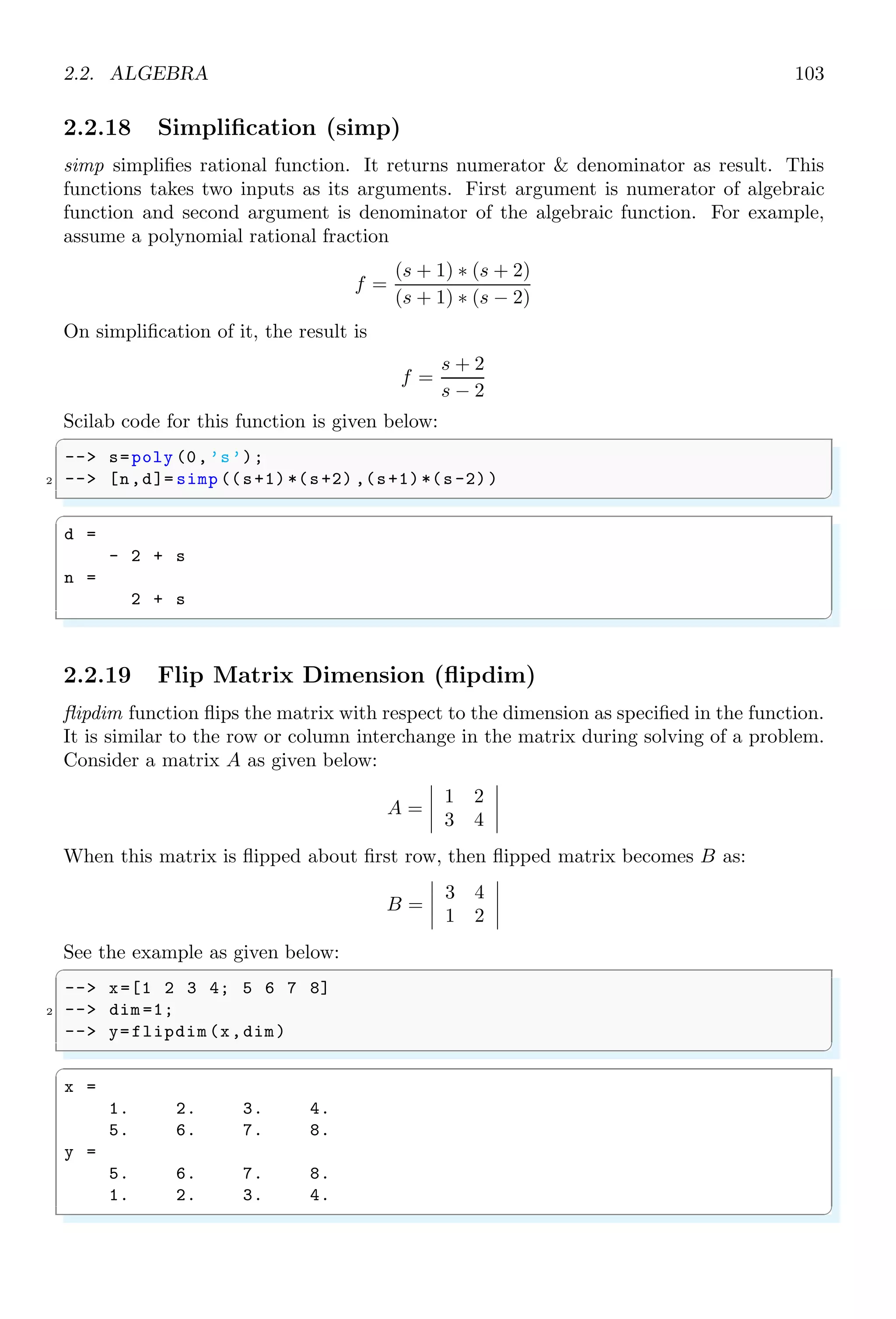
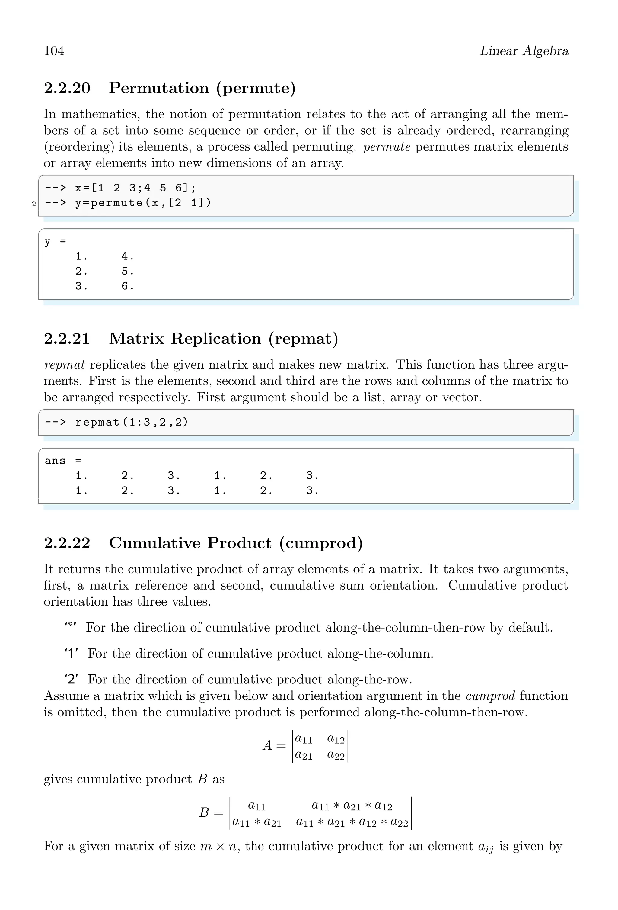
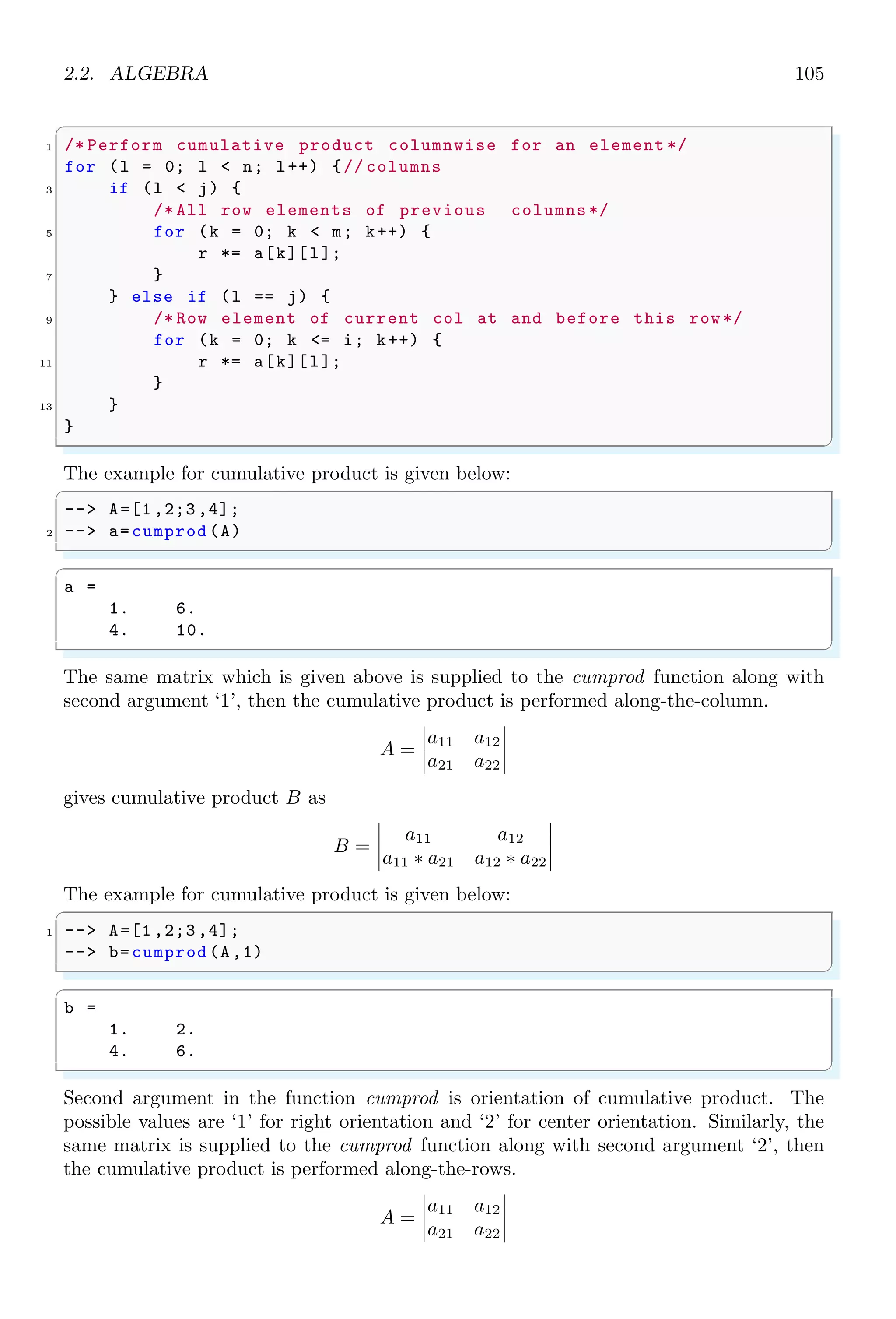
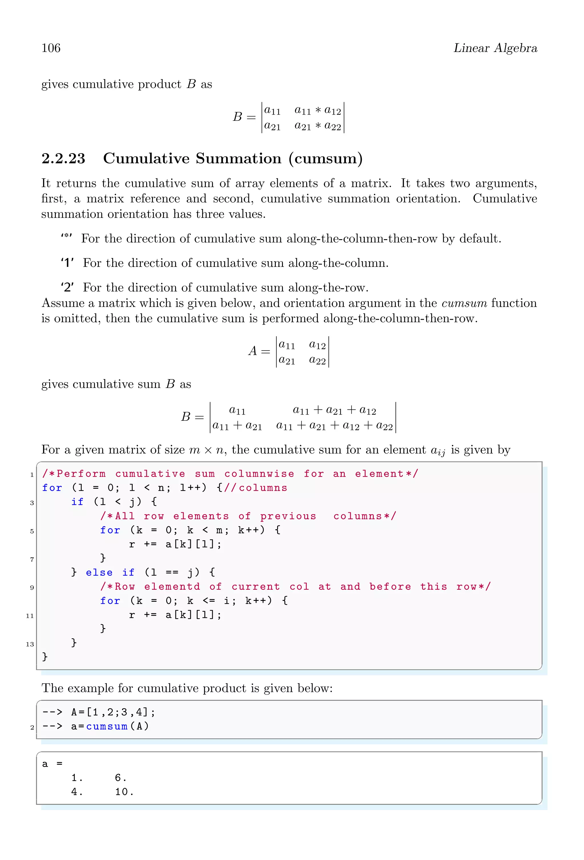
2.2 Algebra
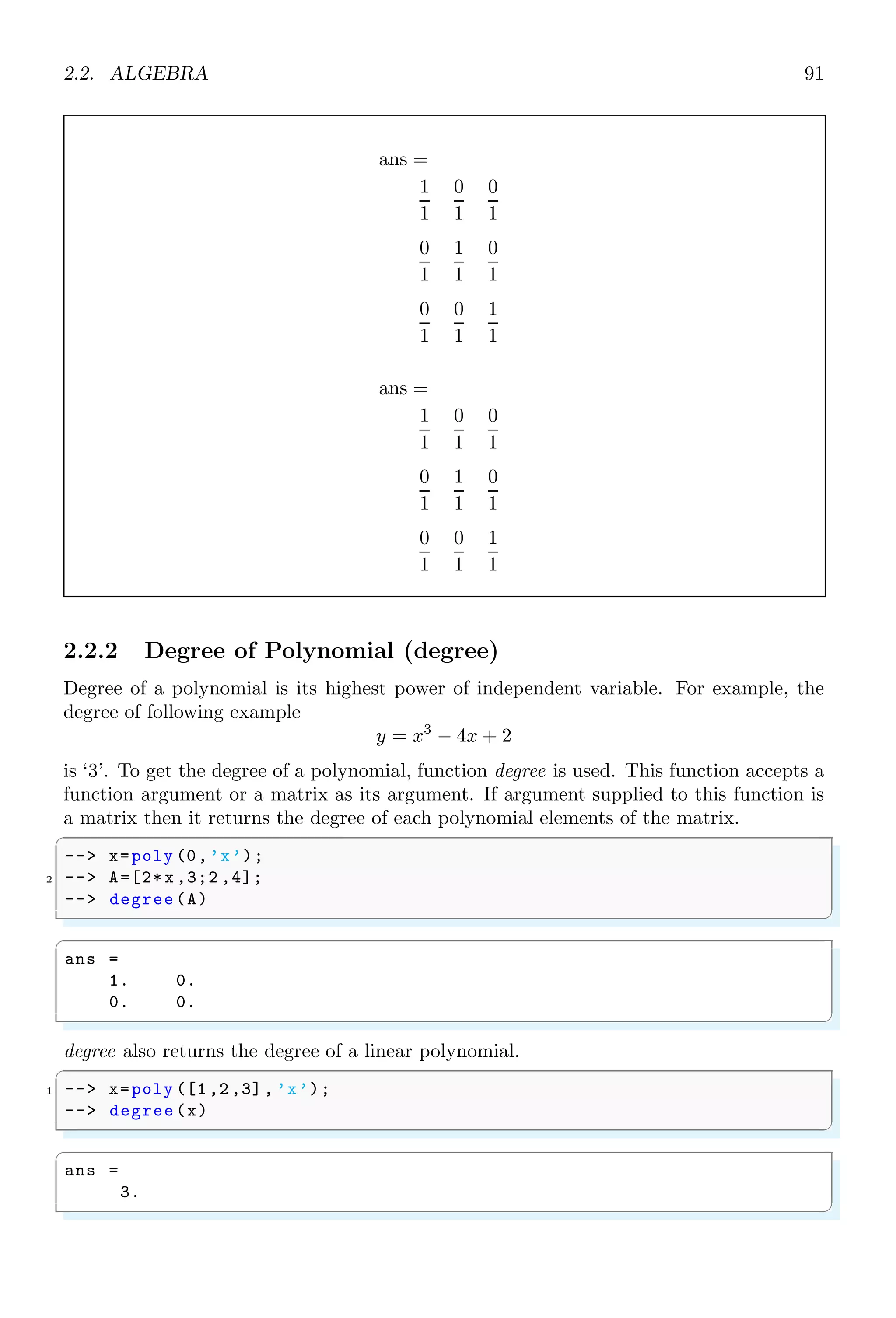
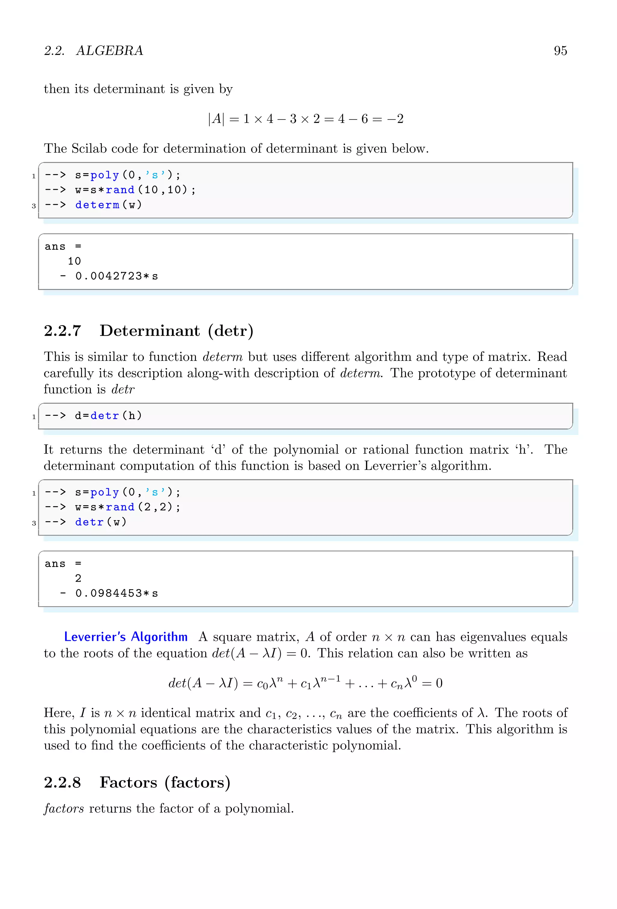
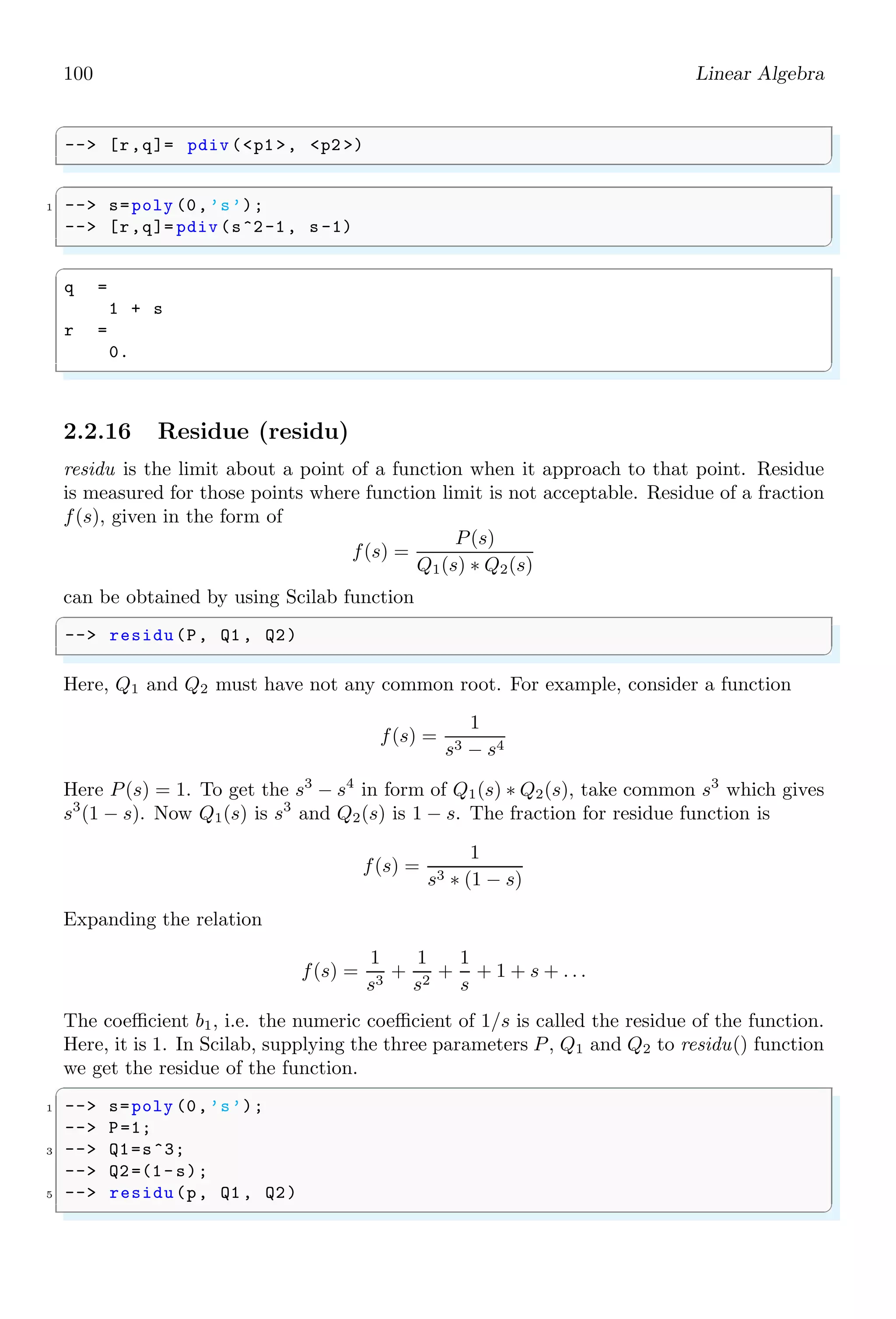
2.2.1 Clean (clean)
This function eliminates all the coefficients with absolute value or relative value in a
polynomial.
✞
-- x=poly (0,’x’);
2 -- w=[x,1,2+x;3+x,2-x,x^2;1 ,2 ,3+x]/3;
-- w*inv(w)
4 -- clean(w*inv(w))
✌
✆](https://image.slidesharecdn.com/scilabhelpbook1of2-220117060625/75/Scilab-help-book-1-of-2-124-2048.jpg)
![2.2. ALGEBRA 91
ans =
1
1
0
1
0
1
0
1
1
1
0
1
0
1
0
1
1
1
ans =
1
1
0
1
0
1
0
1
1
1
0
1
0
1
0
1
1
1
2.2.2 Degree of Polynomial (degree)
Degree of a polynomial is its highest power of independent variable. For example, the
degree of following example
y = x3
− 4x + 2
is ‘3’. To get the degree of a polynomial, function degree is used. This function accepts a
function argument or a matrix as its argument. If argument supplied to this function is
a matrix then it returns the degree of each polynomial elements of the matrix.
✞
-- x=poly (0,’x’);
2 -- A=[2* x,3;2 ,4];
-- degree(A)
✌
✆
✞
ans =
1. 0.
0. 0.
✌
✆
degree also returns the degree of a linear polynomial.
✞
1 -- x=poly ([1,2,3], ’x’);
-- degree(x)
✌
✆
✞
ans =
3.
✌
✆](https://image.slidesharecdn.com/scilabhelpbook1of2-220117060625/75/Scilab-help-book-1-of-2-125-2048.jpg)
![92 Linear Algebra
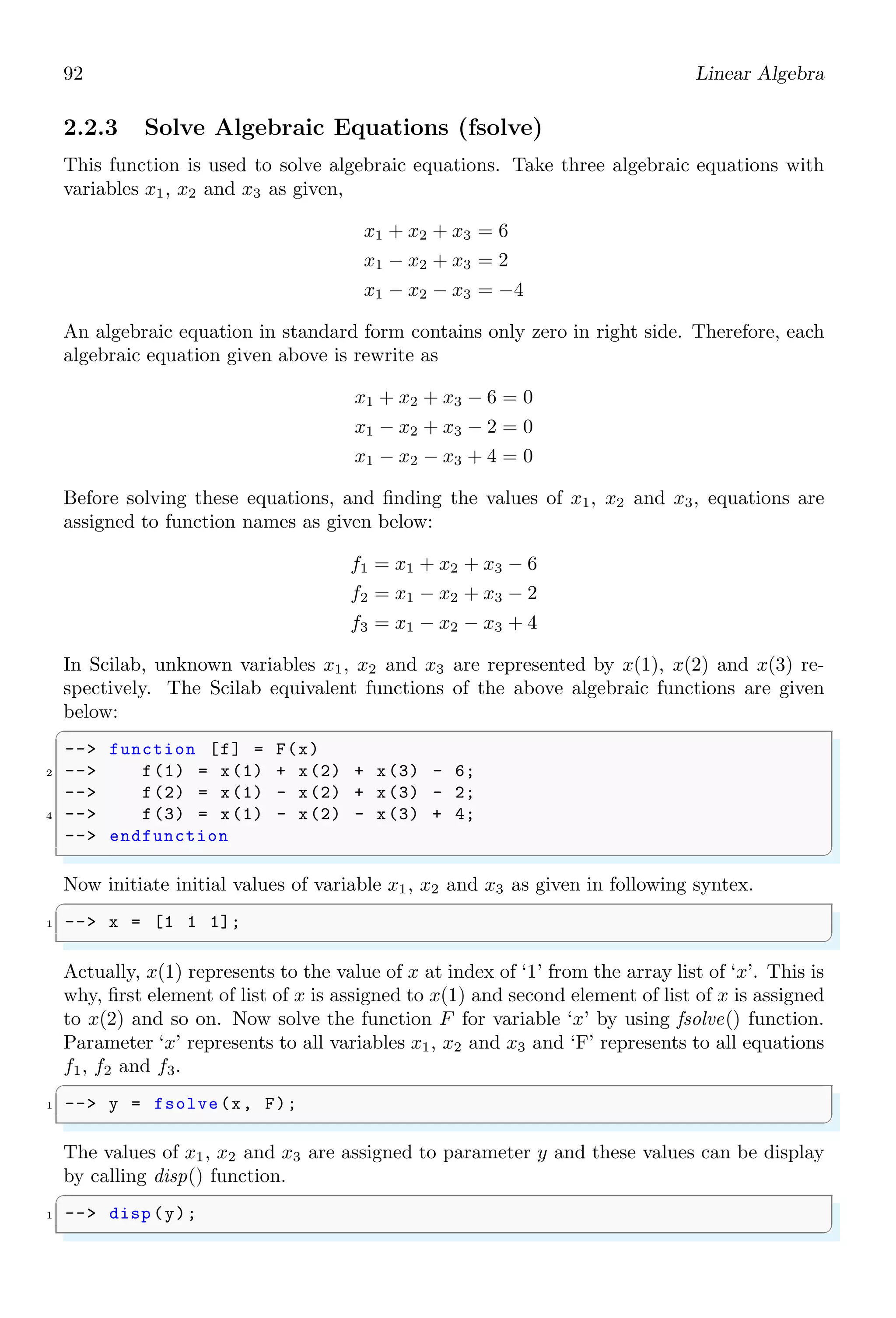
2.2.3 Solve Algebraic Equations (fsolve)
This function is used to solve algebraic equations. Take three algebraic equations with
variables x1, x2 and x3 as given,
x1 + x2 + x3 = 6
x1 − x2 + x3 = 2
x1 − x2 − x3 = −4
An algebraic equation in standard form contains only zero in right side. Therefore, each
algebraic equation given above is rewrite as
x1 + x2 + x3 − 6 = 0
x1 − x2 + x3 − 2 = 0
x1 − x2 − x3 + 4 = 0
Before solving these equations, and finding the values of x1, x2 and x3, equations are
assigned to function names as given below:
f1 = x1 + x2 + x3 − 6
f2 = x1 − x2 + x3 − 2
f3 = x1 − x2 − x3 + 4
In Scilab, unknown variables x1, x2 and x3 are represented by x(1), x(2) and x(3) re-
spectively. The Scilab equivalent functions of the above algebraic functions are given
below:
✞
-- function [f] = F(x)
2 -- f(1) = x(1) + x(2) + x(3) - 6;
-- f(2) = x(1) - x(2) + x(3) - 2;
4 -- f(3) = x(1) - x(2) - x(3) + 4;
-- endfunction
✌
✆
Now initiate initial values of variable x1, x2 and x3 as given in following syntex.
✞
1 -- x = [1 1 1];
✌
✆
Actually, x(1) represents to the value of x at index of ‘1’ from the array list of ‘x’. This is
why, first element of list of x is assigned to x(1) and second element of list of x is assigned
to x(2) and so on. Now solve the function F for variable ‘x’ by using fsolve() function.
Parameter ‘x’ represents to all variables x1, x2 and x3 and ‘F’ represents to all equations
f1, f2 and f3.
✞
1 -- y = fsolve(x, F);
✌
✆
The values of x1, x2 and x3 are assigned to parameter y and these values can be display
by calling disp() function.
✞
1 -- disp (y);
✌
✆](https://image.slidesharecdn.com/scilabhelpbook1of2-220117060625/75/Scilab-help-book-1-of-2-126-2048.jpg)
![2.2. ALGEBRA 93
✞
3. 2. 1.
✌
✆
Solved Problem 2.2 Solve simultaneous equations x + y = 4 and 3x + 3y = 2.
Solution Let x = x(1) and y = x(2). The modified form of given equations are
x(1) + x(2) = 4; 3 × x(1) + 3 × x(2) = 2
The Scilab codes for the given equations is
✞
1 -- function [f] = F(x)
-- f(1) = x(1) + x(2) - 4;
3 -- f(2) = 3*x(1) + 3*x(2) - 2;
-- endfunction
5 -- x = [0 0];
-- y = fsolve(x, F);
7 -- disp (y)
✌
✆
✞
x=71.20891, y= -70.20891
✌
✆
These are solutions of the given equations.
2.2.4 Denominator (denom)
A polynomial fraction is given by
y =
x2
+ 3
x3 − 8
A polynomial fraction is acceptable if its degree of numerator is less than or equals to the
degree of its polynomial. If degree of numerator is larger than its degree of denominator,
then numerator is divide by denominator to convert it into whole and fraction parts.
y =
x4
+ 5x
x3 − 8
= x +
13x
x3 − 8
To get the denominator of a polynomial fraction, function denom is used. The argument
of this function may be either a fraction or a matrix of fractions.
✞
1 -- x=poly (0,’x’);
-- A=[2* x,3;2 ,4];
3 -- denom(A)
✌
✆
✞
ans =
1. 1.
1. 1.
✌
✆
If an element or polynomial term is a fraction number then denom returns the denomi-
nator the fraction.](https://image.slidesharecdn.com/scilabhelpbook1of2-220117060625/75/Scilab-help-book-1-of-2-127-2048.jpg)
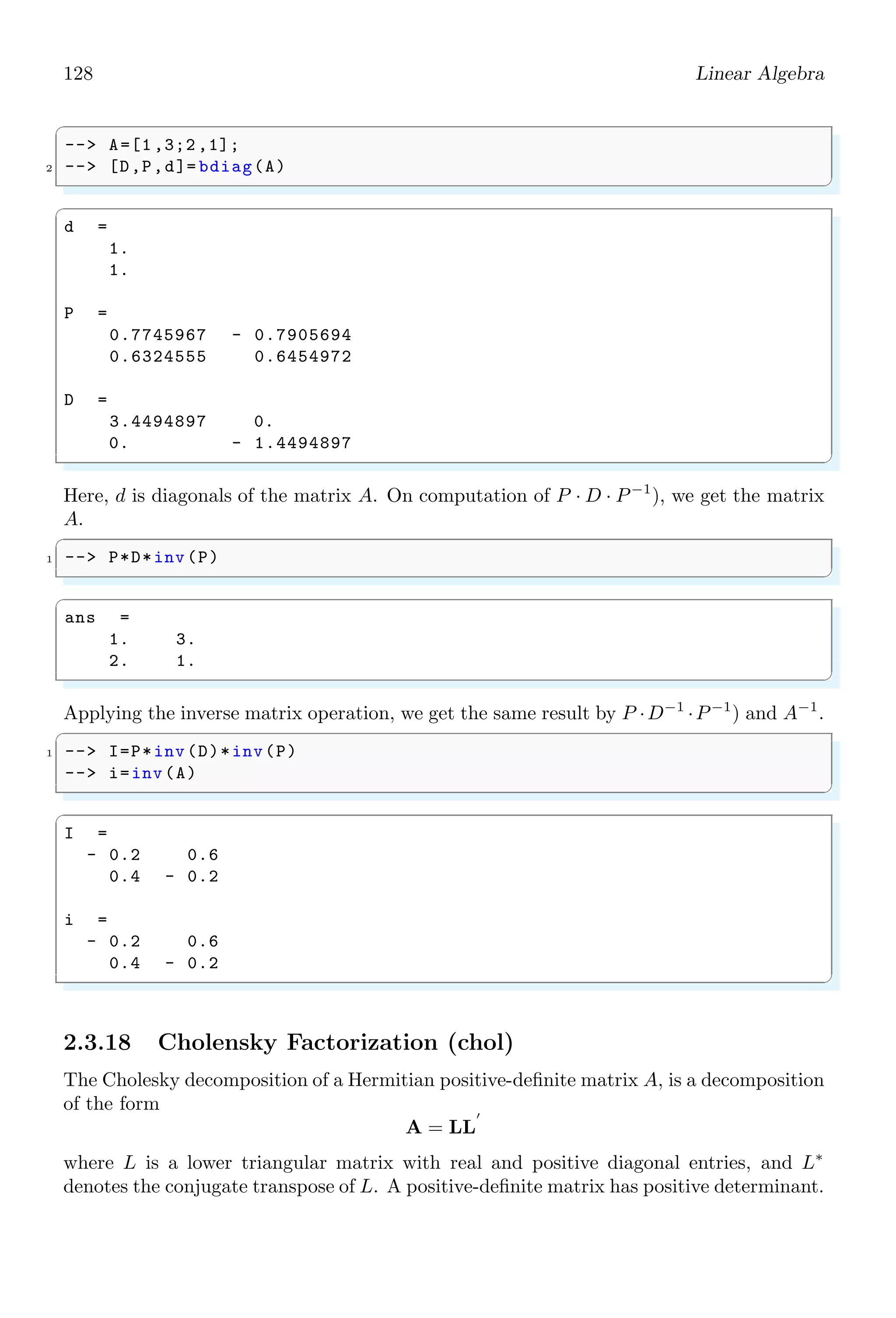
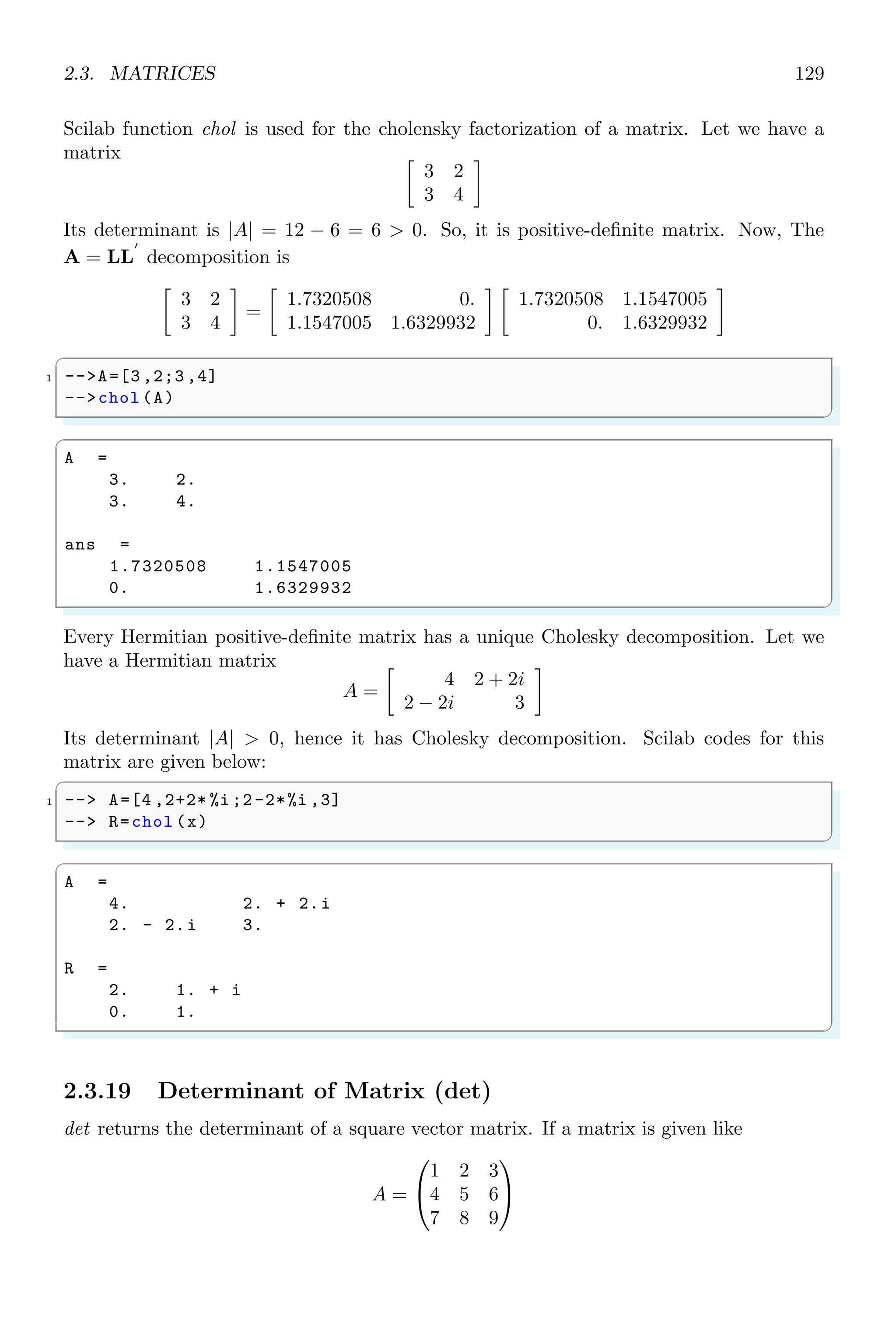
![96 Linear Algebra
✞
1 --n=poly ([1,2,3], ’z’);
--d=poly ([5,6,7], ’z’);
3 --R=syslin(’d’,n,d);
--R1=factors (R,’d’)
5 -- prettyprint (R1)
✌
✆
R1 =
−0.0047619 + 0.0285714z − 0.0523810z2
+ 0.0285714z3
−0.0047619 + 0.0857143z − 0.5095238z2 + z3
2.2.9 Greatest Common Divisor (gcd)
gcd is acronym of greatest common divisor. It is a polynomial or number that can divide
other polynomials without remainders. For example, the gcd of numbers 12 and 18 is
6. The same principle is applicable to the algebraic relations. For example, the greatest
common divisor of algebraic equations (x − 2)(x + 3) and (x − 2)(x + 4) is (x − 2).
✞
1 -- s=poly (0,’s’);
-- p=[s, s*(s+1)^2, 2*s^2+s^3];
3 -- gcd(p)
✌
✆
✞
ans =
s
✌
✆
2.2.10 Inverse of Matrix (invr)
invr returns the inverse matrix. Inverse of a matrix can be obtained if it is convertible.
All square matrices are not convertible. The square matrix which has an inverse is called
convertible or non-singular matrix. A square matrix is convertible when its determinant
is not zero, i.e. det(A) 6= 0. Inverse of a square matrix is given by
A−1
=
Adj(A)
Det(A)
Adj(A) of the matrix A is transpose matrix of the co-factor matrix of matrix A. Co-factor
of a matrix of m × n order in respect of ith
row and jth
column is given by Aij that is
equal to the product of (−1)i×j
and determinant of remaining matrix after eliminating
ith
row and jth
column. Let a matrix is given like
A =
1 2
3 4
The co-factors of the matrix are
a11 = (−1)1+1
× 4; a11 = (−1)1+2
× 3;
a21 = (−1)2+1
× 2; a22 = (−1)2+2
× 1;](https://image.slidesharecdn.com/scilabhelpbook1of2-220117060625/75/Scilab-help-book-1-of-2-130-2048.jpg)
![2.2. ALGEBRA 97
Now co-factors matrix of matrix A is
Acf =
4 −3
−2 1
Now Adj(A) of matrix A is
Adj(A) =
4 −2
−3 1
Now the determinant of the matrix A is
Det(A) = −2
Finally, inverse of matrix A is
A−1
=
Adj(A)
Det(A)
=
−2. 1.
1.5 −0.5
✞
-- a=[1 ,2;3 ,4]
2 -- invr (a)
✌
✆
✞
ans =
- 2. 1.
1.5 - 0.5
✌
✆
2.2.11 Least Common Multiple (lcm)
lcm is acronym of least common multiple. It is the smallest number or polynomial that
can be divided by more than one polynomials. For example 30 is lcm of numbers 5 and
6. Similarly (x − 2)(x + 3) is least common multiple of the factors (x − 2) and (x − 3).
✞
1 -- s=poly (0,’s’);
-- p=[s,s*(s+1) ^2,2*s^2+s^3];
3 -- lcm(p)
✌
✆
ans =
2s2
+ 5s3
+ 4s4
+ s5
2.2.12 LCM By Diagonalization (lcmdiag)
lcmdiag returns the least common multiple of a matrix using diagonal factorization
method.
✞
1 -- s=poly (0,’s’);
-- H=[1/ s,s;1/s^2,2/s];
3 -- [N,D]= lcmdiag(H)
✌
✆](https://image.slidesharecdn.com/scilabhelpbook1of2-220117060625/75/Scilab-help-book-1-of-2-131-2048.jpg)
![98 Linear Algebra
D =
s2
0
0 s
N =
s s2
1 2
2.2.13 Numerator (numer)
numer returns the numerator value of a fraction. A polynomial fraction is given by
y =
x2
+ 3
x3 − 8
A polynomial fraction is acceptable if its degree of numerator is less than or equals to the
degree of its polynomial. If degree of numerator is larger than its degree of denominator,
then numerator is divide by denominator to convert it into whole and fraction parts.
y =
x4
+ 5x
x3 − 8
= x +
13x
x3 − 8
To get the numerator of a polynomial fraction, function numer is used.
✞
1 -- s=poly (0,’s’);
-- numer (2/s)
✌
✆
✞
ans =
2
✌
✆
✞
-- s=poly (0,’s’);
2 -- H=[1/ s,s;1/s^2,2/s];
-- numer(H)
✌
✆
ans =
1 s
1 2](https://image.slidesharecdn.com/scilabhelpbook1of2-220117060625/75/Scilab-help-book-1-of-2-132-2048.jpg)
![2.2. ALGEBRA 99
2.2.14 Polynomial (poly)
Any linear relation of a unknown variable having degree more than ‘2’ is known as poly-
nomials. For example, x3
+ 2x − 3 = 0 is a polynomial of variable x. Degree of the
polynomial is ‘3’. If [1, 2, 3] are the roots of a polynomial then degree of the polynomial
is ‘3’ (No of roots). Each root represents the factor of ‘x’. If x = rn are roots of a
polynomial then
n
Y
i=1
(x − rk) is polynomial of these roots. For given roots [1, 2, 3], factors
of the polynomial are
Roots x = 1 x = 2 x = 3
Factors (x-1) (x-2) (x-3)
Polynomial having these roots is
(x − 1) × (x − 2) × (x − 3) = 0
✞
1 -- x=poly ([1,2,3], ’x’)
✌
✆
ans =
− 6 + 11x − 6x2
+ x3
degree() returns the degree of the polynomial supplied as its argument.
✞
1 -- x=poly ([1,2,3], ’x’);
-- degree(x)
✌
✆
✞
ans =
3.
✌
✆
2.2.15 Polynomial Division (pdiv)
pdiv returns the euclidean division of polynomials. By default, it returns only quotient
value.
✞
-- s=poly (0,’s’);
2 -- pdiv (s^2-1, s^2)
✌
✆
✞
ans =
1
✌
✆
If quotient remainder both are to be found as returned values then this function is used
with return argument as shown in the following example.](https://image.slidesharecdn.com/scilabhelpbook1of2-220117060625/75/Scilab-help-book-1-of-2-133-2048.jpg)
![100 Linear Algebra
✞
-- [r,q]= pdiv (p1 , p2 )
✌
✆
✞
1 -- s=poly (0,’s’);
-- [r,q]= pdiv (s^2-1, s -1)
✌
✆
✞
q =
1 + s
r =
0.
✌
✆
2.2.16 Residue (residu)
residu is the limit about a point of a function when it approach to that point. Residue
is measured for those points where function limit is not acceptable. Residue of a fraction
f(s), given in the form of
f(s) =
P(s)
Q1(s) ∗ Q2(s)
can be obtained by using Scilab function
✞
-- residu(P, Q1 , Q2)
✌
✆
Here, Q1 and Q2 must have not any common root. For example, consider a function
f(s) =
1
s3 − s4
Here P(s) = 1. To get the s3
− s4
in form of Q1(s) ∗ Q2(s), take common s3
which gives
s3
(1 − s). Now Q1(s) is s3
and Q2(s) is 1 − s. The fraction for residue function is
f(s) =
1
s3 ∗ (1 − s)
Expanding the relation
f(s) =
1
s3
+
1
s2
+
1
s
+ 1 + s + . . .
The coefficient b1, i.e. the numeric coefficient of 1/s is called the residue of the function.
Here, it is 1. In Scilab, supplying the three parameters P, Q1 and Q2 to residu() function
we get the residue of the function.
✞
1 -- s=poly (0,’s’);
-- P=1;
3 -- Q1=s^3;
-- Q2=(1- s);
5 -- residu(p, Q1 , Q2)
✌
✆](https://image.slidesharecdn.com/scilabhelpbook1of2-220117060625/75/Scilab-help-book-1-of-2-134-2048.jpg)
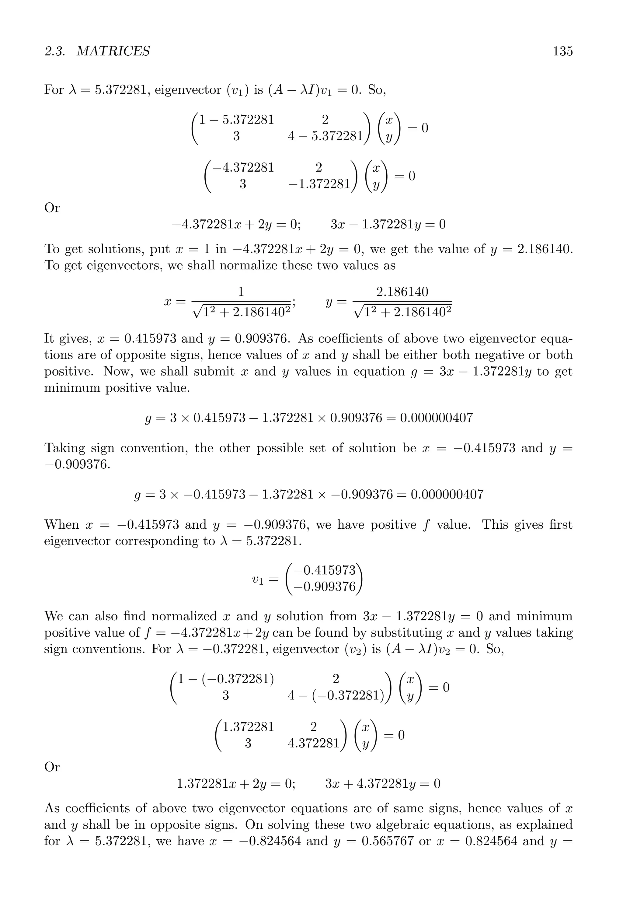
![102 Linear Algebra
✞
1 -- x=poly (0,’x’)
-- roots(x^2 -3 * x + 3)
✌
✆
✞
ans =
1.5 + 0.8660254 i
1.5 - 0.8660254 i
✌
✆
Roots of Polynomials
Roots of higher degree polynomials can be obtained as
✞
1 -- x=poly (0,’x’)
-- roots(x^3 - 6 * x^2 + 11 * x -6)
✌
✆
✞
ans =
3.
2.
1.
✌
✆
All are the real roots. roots function also calculates the complex roots.
✞
-- x=poly (0,’x’)
2 -- roots(x^3 - 6 * x^2 + 11 * x + 1)
✌
✆
✞
ans =
3.04 + 1.50 i
3.04 - 1.50 i
- 0.08
✌
✆
roots returns all the roots of a polynomial function. Roots of a polynomial function
are those possible values which satisfy to the given polynomial to zero. For example,
x2
− 2x + 1 = 0 is a polynomial of degree ‘2’ and is known as quadratic equation. The
roots of this polynomial are x = +1 and x = +1. When in place of ‘x’, 1 is put then
polynomial value is zero.
p(1) = 12
− 2 × 1 + 1 = 0
Roots of a polynomial is obtained either by fraction method or by substitution and re-
duction method.
✞
-- p=poly ([1,2,3], ’s’)
2 -- roots(p)
✌
✆
✞
ans =
3.
2.
1.
✌
✆](https://image.slidesharecdn.com/scilabhelpbook1of2-220117060625/75/Scilab-help-book-1-of-2-136-2048.jpg)
![2.2. ALGEBRA 103
2.2.18 Simplification (simp)
simp simplifies rational function. It returns numerator denominator as result. This
functions takes two inputs as its arguments. First argument is numerator of algebraic
function and second argument is denominator of the algebraic function. For example,
assume a polynomial rational fraction
f =
(s + 1) ∗ (s + 2)
(s + 1) ∗ (s − 2)
On simplification of it, the result is
f =
s + 2
s − 2
Scilab code for this function is given below:
✞
-- s=poly (0,’s’);
2 -- [n,d]= simp ((s+1) *(s+2) ,(s+1)*(s-2))
✌
✆
✞
d =
- 2 + s
n =
2 + s
✌
✆
2.2.19 Flip Matrix Dimension (flipdim)
flipdim function flips the matrix with respect to the dimension as specified in the function.
It is similar to the row or column interchange in the matrix during solving of a problem.
Consider a matrix A as given below:
A =](https://image.slidesharecdn.com/scilabhelpbook1of2-220117060625/75/Scilab-help-book-1-of-2-137-2048.jpg)