This document provides an overview of partial derivatives, which are used to analyze functions with multiple variables. Key topics covered include: - Definitions of limits, continuity, and partial derivatives for multivariable functions. - Directional derivatives and the gradient, which describe the rate of change in a specified direction. - The chain rule for partial derivatives, and implicit differentiation. - Linearization and Taylor series approximations for multivariable functions. - Finding local extrema and optimizing functions, using techniques like classifying critical points.

1. Calculus III (part 2): Partial Derivatives (by Evan Dummit, 2017, v. 2.60)
Contents
2 Partial Derivatives 1
2.1 Limits and Continuity . . . . . . . . . . . . . . . . . . . . . . . . . . . . . . . . . . . . . . . . . . . . 1
2.2 Partial Derivatives . . . . . . . . . . . . . . . . . . . . . . . . . . . . . . . . . . . . . . . . . . . . . . 5
2.3 Directional Derivatives and the Gradient . . . . . . . . . . . . . . . . . . . . . . . . . . . . . . . . . . 7
2.3.1 Tangent Lines and Tangent Planes . . . . . . . . . . . . . . . . . . . . . . . . . . . . . . . . . 10
2.4 The Chain Rule . . . . . . . . . . . . . . . . . . . . . . . . . . . . . . . . . . . . . . . . . . . . . . . . 11
2.4.1 Implicit Dierentiation . . . . . . . . . . . . . . . . . . . . . . . . . . . . . . . . . . . . . . . . 13
2.5 Linearization and Taylor Series . . . . . . . . . . . . . . . . . . . . . . . . . . . . . . . . . . . . . . . 14
2.5.1 Linearization . . . . . . . . . . . . . . . . . . . . . . . . . . . . . . . . . . . . . . . . . . . . . 14
2.5.2 Taylor Series . . . . . . . . . . . . . . . . . . . . . . . . . . . . . . . . . . . . . . . . . . . . . 16
2.6 Local Extreme Points and Optimization . . . . . . . . . . . . . . . . . . . . . . . . . . . . . . . . . . 17
2.6.1 Critical Points, Minima and Maxima, Saddle Points, Classifying Critical Points . . . . . . . . 17
2.6.2 Optimization of a Function on a Region . . . . . . . . . . . . . . . . . . . . . . . . . . . . . . 21
2.7 Lagrange Multipliers and Constrained Optimization . . . . . . . . . . . . . . . . . . . . . . . . . . . 22
2 Partial Derivatives
In this chapter, we develop the theory of dierentiation for functions of several variables, and discuss applications to
optimization and nding local extreme points. The development of these topics is very similar to that of one-variable
calculus, save for some additional complexities due to the presence of extra variables.
2.1 Limits and Continuity
• In order to talk about derivatives in the multivariable setting, we rst need to establish what limits and
continuity should mean.
• Denition: A function f(x, y) has the limit L as (x, y) → (a, b), written as lim
(x,y)→(a,b)
f(x, y) = L, if, for any
0 (no matter how small) there exists a δ 0 (depending on ) with the property that for all (x, y) with
0 (x − a)2 + (y − b)2 δ, we have that |f(x, y) − L| .
◦ The square root might be a little bit unsettling. But it is just a statement about distance: saying that
0 (x − a)2 + (y − b)2 δ just means that the point (x, y) is within a distance δ of the point (a, b).
◦ Compare this denition to the formal denition of limit for a function of one variable: A function f(x)
has the limit L as x → a, written as lim
x→a
f(x) = L, if, for any 0 (no matter how small) there exists a
δ 0 (depending on ) with the property that for all 0 |x − a| δ, we have that |f(x) − L| .
◦ The multivariable denition and single-variable denitions both mean the same intuitive thing: suppose
you claim that the function f has a limit L, as we get close to some point P. In order to prove to me
that the function really does have that limit, I challenge you by handing you some value 0, and I
want you to give me some value of δ, with the property that f(x) is always within of the limit value L,
for all the points which are within δ of P.
1

2. ◦ Remark: We can also dene limits of functions of more than two variables. The denition is very similar
in all of those cases: for example, to talk about a limit of a function f(x, y, z) as (x, y, z) → (a, b, c),
the only changes are to write (x, y, z) in place of (x, y), to write (a, b, c) in place of (a, b), and to write
(x − a)2 + (y − b)2 + (z − c)2 in place of (x − a)2 + (y − b)2.
• Denition: A function f(x, y) is continuous at a point (a, b) if lim
(x,y)→(a,b)
f(x, y) is equal to the value f(a, b).
In other words, a function is continuous if its value equals its limit.
◦ Continuous functions of several variables are just like continuous functions of a single variable: they
don't have jumps and they do not blow up to ∞ or −∞.
• Like the one-variable case, the formal denition of limit is cumbersome and generally not easy to use, even
for simple functions. Here are a few simple examples, just to give some idea of the proofs:
◦ Example: Show that lim
(x,y)→(a,b)
c = c, for any constant c.
∗ In this case it turns out that we can take any positive value of δ at all. Let's try δ = 1.
∗ Suppose we are given 0. We want to verify that 0 (x − a)2 + (y − b)2 1 will always imply
that |c − c| .
∗ But this is clearly true, because |c − c| = 0, and we assumed that 0 .
∗ So (as certainly ought to be true!) the limit of a constant function is that constant.
◦ Example: Show that lim
(x,y)→(2,3)
x = 2.
∗ Suppose we are given 0. We want to nd δ 0 so that 0 (x − 2)2 + (y − 3)2 δ will always
imply that |x − 2| .
∗ We claim that taking δ = will work.
∗ To see that this choice works, suppose that 0 (x − 2)2 + (y − 3)2 , and square everything.
∗ We obtain 0 (x − 2)2
+ (y − 3)2
2
.
∗ Now since (y − 3)2
is the square of the real number y − 3, we see in particular that 0 ≤ (y − 3)2
.
∗ Thus we can write (x − 2)2
≤ (x − 2)2
+ (y − 3)2
2
, so that (x − 2)2
2
.
∗ Now taking the square root shows |x − 2| | |.
∗ However, since 0 this just says |x − 2| , which is exactly the desired result.
◦ Remark: Using essentially the same argument, one can show that lim
(x,y)→(a,b)
x = a, and also (by inter-
changing the roles of x and y) that lim
(x,y)→(a,b)
y = b, which means that x and y are continuous functions.
• As we would hope, all of the properties of one-variable limits also hold for multiple-variable limits; even the
proofs are essentially the same. Specically, let f(x, y) and g(x, y) be functions satisfying lim
(x,y)→(a,b)
f(x, y) = Lf
and lim
(x,y)→(a,b)
g(x, y) = Lg. Then the following properties hold:
◦ The addition rule: lim
(x,y)→(a,b)
[f(x, y) + g(x, y)] = Lf + Lg.
◦ The subtraction rule: lim
(x,y)→(a,b)
[f(x, y) − g(x, y)] = Lf − Lg.
◦ The multiplication rule: lim
(x,y)→(a,b)
[f(x, y) · g(x, y)] = Lf · Lg.
◦ The division rule: lim
(x,y)→(a,b)
f(x, y)
g(x, y)
=
Lf
Lg
, provided that Lg is not zero.
◦ The exponentiation rule: lim
(x,y)→(a,b)
[f(x, y)]
a
= (Lf )
a
, where a is any positive real number. (It also holds
when a is negative or zero, provided Lf is positive, in order for both sides to be real numbers.)
◦ The squeeze rule: If f(x, y) ≤ g(x, y) ≤ h(x, y) and lim
(x,y)→(a,b)
f(x, y) = lim
(x,y)→(a,b)
h(x, y) = L (meaning
that both limits exist and are equal to L) then lim
(x,y)→(a,b)
g(x, y) = L as well.
2

3. • Here are some examples of limits that can be evaluated using the limit rules:
◦ Example: Evaluate lim
(x,y)→(1,1)
x2
− y
x + y
.
∗ By the limit rules we have lim
(x,y)→(1,1)
x2
− y = lim
(x,y)→(1,1)
x2
− lim
(x,y)→(1,1)
[y] = 12
− 1 = 0 and
lim
(x,y)→(1,1)
[x + y] = lim
(x,y)→(1,1)
[x] + lim
(x,y)→(1,1)
[y] = 1 + 1 = 2.
∗ Then lim
(x,y)→(1,1)
x2
− y
x + y
=
lim
(x,y)→(1,1)
x2
− y
lim
(x,y)→(1,1)
[x + y]
=
0
2
= 0 .
◦ Example: Evaluate lim
(x,y)→(0,0)
x y sin
1
x − y
.
∗ If we try plugging in (x, y) = (0, 0) then we obtain 0 · 0 · sin
1
0
, which is undened: the issue is
the sine term, which also prevents us from using the multiplication property.
∗ Instead, we try using the squeeze rule: because sine is between −1 and +1, we have the inequalities
− |xy| ≤ x y sin
1
x − y
≤ |x y|.
∗ We can compute that lim
(x,y)→(0,0)
|x y| = lim
(x,y)→(0,0)
|x| · lim
(x,y)→(0,0)
|y| = 0 · 0 = 0.
∗ Therefore, applying the squeeze rule, with f(x, y) = − |x y|, g(x, y) = x y sin
1
x − y
, and h(x, y) =
|x y|, yields lim
(x,y)→(0,0)
x y sin
1
x − y
= 0 .
◦ Example: Evaluate lim
(x,y)→(0,0)
x5
+ y4
x4 + y2
.
∗ We split the limit apart, and compute lim
(x,y)→(0,0)
x5
x4 + y2
and lim
(x,y)→(0,0)
y4
x4 + y2
separately.
∗ We have
x5
x4 + y2
≤
x5
x4
= |x|, so since lim
(x,y)→(0,0)
|x| → 0, by the squeeze rule we see lim
(x,y)→(0,0)
x5
x4 + y2
= 0.
∗ Similarly,
y4
x4 + y2
≤
y4
y2
= y2
, so since lim
(x,y)→(0,0)
y2
→ 0, by the squeeze rule we see
lim
(x,y)→(0,0)
y4
x4 + y2
= 0.
∗ Thus, by the sum rule, we see lim
(x,y)→(0,0)
x5
+ y4
x4 + y2
= 0.
• Using the limit rules and some of the basic limit evaluations we can establish that the usual slate of functions
is continuous:
◦ Any polynomial in x and y is continuous everywhere.
◦ The exponential, sine, and cosine of any continuous function are all continuous everywhere.
◦ The logarithm of a positive continuous function is continuous.
◦ Any quotient of polynomials
p(x, y)
q(x, y)
is continuous everywhere that the denominator is nonzero.
• For one-variable limits, we also have a notion of one-sided limits, namely, the limits that approach the target
point either from above or from below. In the multiple-variable case, there are many more paths along which
we can approach our target point.
◦ For example, if our target point is the origin (0, 0), then we could approach along the positive x-axis,
or the positive y-axis, or along any line through the origin or along the curve y = x2
, or any other
continuous curve that approaches the origin.
3

4. • As with limits in a single variable, if limits from dierent directions have dierent values, then the overall
limit does not exist. More precisely:
• Test (Two Paths Test): Let f(x, y) be a function of two variables and (a, b) be a point. If there are two
continuous paths passing through the point (a, b) such that f has dierent limits as (x, y) → (a, b) along the
two paths, then lim
(x,y)→(a,b)
f(x, y) does not exist.
◦ The proof is essentially just the denition of limit: if the limit existed, then close to (a, b), the function
would have to stay within a very small range. But if there are two paths through (a, b) where the function
approaches dierent values, the limit cannot exist.
◦ To apply the test, we try to generate some parametric curves (x(t), y(t)) that pass through the point
(a, b) when t = t0, and compute lim
t→t0
f (x(t), y(t)) as a limit in the single variable t.
• Example: Show that lim
(x,y)→(0,0)
xy
x2 + y2
does not exist.
◦ We try some simple paths: along the path (x, y) = (t, 0) as t → 0 the limit becomes lim
t→0
t · 0
t2 + 02
= lim
t→0
0
t2
= 0.
◦ Along the path (x, y) = (0, t) as t → 0 we have lim
t→0
0 · t
02 + t2
== lim
t→0
0 · t
0 + t2
= lim
t→0
0
t2
= 0.
◦ Along these two paths the limits are equal. But this does not show the existence of the limit lim
(x,y)→(0,0)
xy
x2 + y2
.
◦ Let's try along the path (x, y) = (t, t): the limit then becomes lim
t→0
t2
t2 + t2
= lim
t→0
1
2
=
1
2
.
◦ Thus, along the two paths (x, y) = (0, t) and (x, y) = (t, t), the function has dierent limits as (x, y) →
(0, 0). Hence the limit does not exist.
◦ Below on the left is a plot of the function near (0, 0):
• Example: Show that lim
(x,y)→(0,0)
x2
y
x4 + y2
does not exist. (Plotted above, on the right.)
◦ Along (x, y) = (0, t) the limit is lim
t→0
0 · t
0 + t2
= lim
t→0
0
t2
= 0.
◦ Along (x, y) = (t, t2
) the limit is lim
t→0
t2
· t2
t4 + t4
= lim
t→0
t4
2t4
=
1
2
.
◦ Along these two paths the limit has dierent values, so the general limit does not exist.
◦ Remark: If we try (x, y) = (t, mt) for an arbitrary m, we get lim
t→0
t(mt)2
t2 + (mt)4
= lim
t→0
m2
t3
t2 + m4t4
= lim
t→0
m2
t
1 + m4t2
=
0, since
m2
t
1 + m4t2
→ 0 as t → 0.
∗ So we see that along every line through the origin (including x = 0, which we analyzed above), the
function has the limit 0. Nevertheless, the limit does not exist!
4

5. 2.2 Partial Derivatives
• Partial derivatives are nothing but the usual notion of dierentiation applied to functions of more than one
variable. However, since we now have more than one variable, we also have more than one natural way to
compute a derivative.
• Denition: For a function f(x, y) of two variables, we dene the partial derivative of f with respect to x as
∂f
∂x
= fx = lim
h→0
f(x + h, y) − f(x, y)
h
and the partial derivative of f with respect to y as
∂f
∂y
= fy = lim
h→0
f(x, y + h) − f(x, y)
h
.
◦ Notation: In multivariable calculus, we use the symbol ∂ (typically pronounced either like the letter d or
as del) to denote taking a derivative, in contrast to single-variable calculus where we use the symbol d.
◦ We will frequently use both notations
∂f
∂y
and fy to denote partial derivatives: we generally use the
dierence quotient notation when we want to emphasize a formal property of a derivative, and the
subscript notation when we want to save space.
◦ Geometrically, the partial derivative fx captures how fast the function f is changing in the x-direction,
and fy captures how fast f is changing in the y-direction.
• To evaluate a partial derivative of the function f with respect to x, we need only pretend that all the other
variables (i.e., everything except x) that f depends on are constants, and then just evaluate the derivative of
f with respect to x as a normal one-variable derivative.
◦ All of the derivative rules (the Product Rule, Quotient Rule, Chain Rule, etc.) from one-variable calculus
still hold: there will just be extra variables oating around.
• Example: Find fx and fy for f(x, y) = x3
y2
+ ex
.
◦ For fx, we treat y as a constant and x as the variable. Thus, we see that fx = 3x2
· y2
+ ex
.
◦ Similarly, to nd fy, we instead treat x as a constant and y as the variable, to get fy = x3
· 2y + 0 = 2x3
y .
(Note in particular that the derivative of ex
with respect to y is zero.)
• Example: Find fx and fy for f(x, y) = ln(x2
+ y2
).
◦ For fx, we treat y as a constant and x as the variable. We can apply the Chain Rule to get fx =
2x
x2 + y2
,
since the derivative of the inner function x2
+ y2
with respect to x is 2x.
◦ Similarly, we can use the Chain Rule to nd the partial derivative fy =
2y
x2 + y2
.
• Example: Find fx and fy for f(x, y) =
ex y
x2 + x
.
◦ For fx we apply the Quotient Rule: fx =
∂
∂x [exy
] · (x2
+ x) − exy
· ∂
∂x x2
+ x
(x2 + x)2
. Then we can evaluate
the derivatives in the numerator to get fx =
(y exy
) · (x2
+ x) − exy
· (2x + 1)
(x2 + x)2
.
◦ For fy, the calculation is easier because the denominator is not a function of y. So in this case, we just
need to use the Chain Rule to see that fy =
1
x2 + x
· (x exy
) .
5

6. • We can equally well generalize partial derivatives to functions of more than two variables: for each input
variable, we get a partial derivative with respect to that variable. The procedure remains the same: treat all
variables except the variable of interest as constants, and then dierentiate with respect to the variable of
interest.
• Example: Find fx, fy, and fz for f(x, y, z) = y z e2x2
−y
.
◦ By the Chain Rule we have fx = y z · e2x2
−y
· 4x . (We don't need the Product Rule for fx since y and
z are constants.)
◦ For fy we need to use the Product Rule since f is a product of two nonconstant functions of y. We get
fy = z · e2x2
−y
+ y z · ∂
∂y e2x2
−y
, and then using the Chain Rule gives fy = z e2x2
−y
− y z · e2x2
−y
.
◦ For fz, all of the terms except for z are constants, so we have fz = y e2x2
−y
.
• Like in the one-variable case, we also have higher-order partial derivatives, obtained by taking a partial
derivative of a partial derivative.
◦ For a function of two variables, there are four second-order partial derivatives fxx = ∂
∂x [fx], fxy = ∂
∂y [fx],
fyx = ∂
∂x [fy], and fyy = ∂
∂y [fy].
◦ Remark: Partial derivatives in subscript notation are applied left-to-right, while partial derivatives in
dierential operator notation are applied right-to-left. (In practice, the order of the partial derivatives
rarely matters, as we will see.)
• Example: Find the second-order partial derivatives fxx, fxy, fyx, and fyy for f(x, y) = x3
y4
+ y e2x
.
◦ First, we have fx = 3x2
y4
+ 2y e2x
and fy = 4x3
y3
+ e2x
.
◦ Then we have fxx = ∂
∂x 3x2
y4
+ 2y e2x
= 6xy4
+ 4y e2x
and fxy = ∂
∂y 3x2
y4
+ 2y e2x
= 12x2
y3
+ 2e2x
.
◦ Also we have fyx = ∂
∂x 4x3
y3
+ e2x
= 12x2
y3
+ 2e2x
and fyy = ∂
∂y 4x3
y3
+ e2x
= 12x3
y2
.
• Notice that fxy = fyx for the function in the example above. This is not an accident:
• Theorem (Clairaut): If both partial derivatives fxy and fyx are continuous, then they are equal.
◦ In other words, these mixed partials are always equal, so there are really only three second-order partial
derivatives.
◦ This theorem can be proven using the limit denition of derivative and the Mean Value Theorem, but
the details are unenlightening.
• We can continue on and take higher-order partial derivatives. For example, a function f(x, y) has eight
third-order partial derivatives: fxxx, fxxy, fxyx, fxyy, fyxx, fyxy, fyyx, and fyyy.
◦ By Clairaut's Theorem, we can reorder the partial derivatives any way we want (if they are continuous,
which is almost always the case). Thus, fxxy = fxyx = fyxx, and fxyy = fyxy = fyyx.
◦ So there are really only four third-order partial derivatives: fxxx, fxxy, fxyy, fyyy.
• Example: Find the third-order partial derivatives fxxx, fxxy, fxyy, fyyy for f(x, y) = x4
y2
+ x3
ey
.
◦ First, we have fx = 4x3
y2
+ 3x2
ey
and fy = 2x4
y + x3
ey
.
◦ Next, fxx = 12x2
y2
+ 6xey
, fxy = 8x3
y + 3x2
ey
, and fyy = 2x4
+ x3
ey
.
◦ Finally, fxxx = 24xy2
+ 6ey
, fxxy = 24x2
y + 6xey
, fxyy = 8x3
+ 3x2
ey
, and fyyy = x3
ey
.
6

7. 2.3 Directional Derivatives and the Gradient
• Aside from the partial derivatives, there is another notion of derivative for a function of several variables. If,
for example, f(x, y) is a function of two variables, then the partial derivatives fx and fy measure how much
f is changing in the direction of the x-axis and in the direction of the y-axis, respectively. However, there
is no reason we couldn't ask for the rate of change of f in any direction, not just in the direction of one of
the coordinate axes. This leads to what is called the directional derivative:
• Denition: If v = vx, vy is a unit vector, then the directional derivative of f(x, y) in the direction of v at
(x, y), denoted Dv(f)(x, y), is dened to be the limit Dv(f)(x, y) = lim
h→0
f (x + h vx, y + h vy) − f (x, y)
h
,
provided that the limit exists.
◦ The corresponding limits when f has more variables are analogous.
◦ Important Note: In the denition of directional derivative, the vector v is a unit vector. We sometimes
will speak of the directional derivative of a function in the direction of a vector w whose length is not 1:
what we mean by this is the directional derivative in the direction of the unit vector
w
||w||
pointing the
same direction as w.
◦ The limit in the denition is explicit, but a little bit hard to understand. If we write things in vector
notation, with x = x, y , then the denition is clearer: it becomes Dv(f)(x) = lim
h→0
f(x + h v) − f(x)
h
.
(Compare it to the denition of the derivative of a function of one variable.)
◦ Although it may not be immediately obvious, the directional derivative is very closely related to the
partial derivatives:
∗ If we take v = 1, 0 , the unit vector in the direction of the x-axis, the denition reduces to
lim
h→0
f(x + h, y) − f(x, y)
h
= fx(x, y).
∗ If we take v = 0, 1 , the unit vector in the direction of the y-axis, the denition reduces to
lim
h→0
f(x, y + h) − f(x, y)
h
= fy(x, y).
∗ So we see that the directional derivative encompasses both of the usual partial derivatives as special
cases for particular direction vectors v.
• It is cumbersome to apply the denition to compute directional derivatives. Fortunately, there is an easier
way to compute them, using partial derivatives and a vector called the gradient.
• Denition: The gradient of a function f(x, y, z), denoted f, is dened to be the vector-valued function
f(x, y, z) = fx(x, y, z), fy(x, y, z), fz(x, y, z) .
◦ Note: The symbol is called nabla, and is pronounced either as nabla or as del.
◦ If f is a function of some other number of variables, the gradient is dened analogously: the component
of the vector in any coordinate is the partial derivative f of f with respect to . Thus, for a function
g(x, y) we have g = gx, gy .
◦ Note that the gradient of f is a vector-valued function: it takes the same number of arguments as f
does, and outputs a vector in the same number of coordinates.
◦ Example: For f(x, y, z) = x2
+ y2
+ z2
, we have f(x, y, z) = fx, fy, fz = 2x, 2y, 2z .
◦ Example: For f(x, y) = x2
cos(y), we have f(x, y) = fx, fy = 2x cos(y), −x2
sin(y) .
• Theorem (Gradient and Directional Derivatives): If v is any unit vector, and f is a function all of whose partial
derivatives are continuous, then the directional derivative Dvf satises Dvf = f · v . In other words, the
directional derivative of f in the direction of v is equal to the dot product of f with the vector v.
◦ Proof (for functions f(x, y) of two variables): If vx = 0 then the directional derivative is the x-partial
(or its negative), and if vy = 0 then the directional derivative is the y-partial (or its negative), and the
result is true.
7

8. ∗ If vx and vy are both nonzero, then we can write
Dv(f)(x, y) = lim
h→0
f(x + h vx, y + h vy) − f(x, y)
h
,
= lim
h→0
f(x + h vx, y + h vy) − f(x, y + h vy)
h
+
f(x, y + h vy) − f(x, y)
h
= lim
h→0
f(x + h vx, y + h vy) − f(x, y + h vy)
h vx
vx +
f(x, y + h vy) − f(x, y)
h vy
vy
= vx lim
h→0
f(x + h vx, y + h vy) − f(x, y + h vy)
h vx
+ vy lim
h→0
f(x, y + h vy) − f(x, y)
h vy
∗ By continuity, one can check that the quotient
f(x + h vx, y + h vy) − f(x, y + h vy)
h vx
tends to the
partial derivative
∂f
∂x
(x, y) as h → 0, and that the second quotient
f(x, y + h vy) − f(x, y)
h vy
equals
the partial derivative
∂f
∂y
(x, y) as h → 0.
∗ Putting these two values into the expression yields Dv(f)(x, y) = vx
∂f
∂x
+vy
∂f
∂y
= vx, vy · fx, fy =
v · f, as claimed.
◦ The proof for functions of more than two variables is essentially the same as for functions of two variables.
• Example: If v =
3
5
,
4
5
, and f(x, y) = 2x + y, nd the directional derivative of f in the direction of v at
(1, 2), both from the denition of directional derivative and from the gradient theorem.
◦ Since v is a unit vector, the denition says that
Dv(f)(1, 2) = lim
h→0
f(x + h vx, y + h vy) − f(x, y)
h
= lim
h→0
f 1 +
3
5
h, 2 +
4
5
h − f(x, y)
h
= lim
h→0
2(1 +
3
5
h) + (2 +
4
5
h) − [2 · 1 + 2]
h
= lim
h→0
2 +
6
5
h + 2 +
4
5
h − 4
h
= lim
h→0
6
5
h +
4
5
h
h
=
6
5
+
4
5
= 2 .
◦ To compute the answer using the gradient, we immediately have fx = 2 and fy = 1, so f = 2, 1 .
Then the theorem says Dvf = f · v = 2, 1 ·
3
5
,
4
5
=
6
5
+
4
5
= 2 .
◦ Observe how much easier it was to use the gradient to compute the directional derivative!
• Example: Find the rate of change of the function f(x, y, z) = exyz
at the point (x, y, z) = (1, 1, 1) in the
direction of the vector w = −2, 1, 2 .
◦ Note that w is not a unit vector, so we must normalize it: since ||w|| = (−2)2 + 12 + 22 = 3, we take
v =
w
||w||
= −
2
3
,
1
3
,
2
3
.
◦ Furthermore, we compute f = yz exyz
, xz exyz
, xy exyz
, so f(−2, 1, 2) = 2e−4
, −4e−4
, −2e−4
.
◦ Then the desired rate of change is Dvf = f · v = −
2
3
(2e−4
) +
1
3
(−4e−4
) +
2
3
(−2e−4
) = −4e−4
.
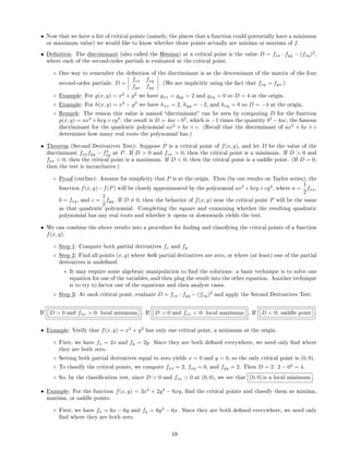
• From the gradient theorem for computing directional derivatives, we can deduce several corollaries:
8

9. ◦ Corollary 1: The maximum value of the directional derivative Dvf occurs when v is a unit vector pointing
in the direction of f, if f = 0, and the maximum value is || f||.
∗ In other words, the gradient points in the direction where f is increasing most rapidly.
◦ Corollary 2: The minimum value of the directional derivative Dvf occurs when v is a unit vector pointing
the opposite direction of f, if f = 0, and the minimum value is − || f||.
∗ In other words, the gradient points in the opposite direction from where f is decreasing most rapidly.
◦ Corollary 3: The directional derivative Dvf is zero if and only if v is orthogonal to the gradient f.
◦ Proof (of all corollaries): If v is a unit vector, then the directional derivative satises Dvf = f · v =
|| f|| ||v|| cos(θ), where θ is the angle between f and v.
∗ We know that || f|| is a xed nonnegative number, and ||v|| = 1. So if we change the direction of
v, the only quantity in || f|| ||v|| cos(θ) that changes is cos(θ).
∗ So, the maximum value of f ·v occurs when cos(θ) = 1, which is to say, when f and v are parallel
and point in the same direction. The maximum value is then just || f||.
∗ Also, the minimum value of f · v occurs when cos(θ) = −1, which is to say, when f and v are
parallel and point in opposite directions. The minimum value is then just − || f||.
∗ Finally, Dvf is zero if and only if f = 0 or θ =
π
2
, and both of these statements are equivalent to
saying that f and v are orthogonal.
• Example: For the function f(x, y) = x2
+ y2
, in which direction is the function increasing the fastest at
(x, y) = (3, 4), and how fast is it increasing? In which direction is it decreasing the fastest, and how fast?
◦ The corollaries tell us that the function is increasing the fastest in the direction of the gradient and
decreasing the fastest in the direction opposite to the gradient, and the corresponding maximum rate of
increase (or decrease) is the magnitude of the gradient.
◦ We have fx = 2x and fy = 2y so f = 2x, 2y , and f(3, 4) = 6, 8 .
◦ Since || f(3, 4)|| =
√
62 + 82 = 10, we see that the maximum value of the directional derivative Dvf is
10 and occurs in the direction of
6, 8
10
=
3
5
,
4
5
.
◦ Likewise, the minimum value of Dvf is −10 and occurs in the direction of −
6, 8
10
= −
3
5
, −
4
5
.
• Example: For the function f(x, y, z) = x3
+ y3
+ 2z3
, in which direction is the function increasing the fastest
at (x, y, z) = (2, −2, 1), and how fast is it increasing? In which direction is it decreasing the fastest, and how
fast?
◦ As above, the function is increasing the fastest in the direction of the gradient and decreasing the fastest
in the direction opposite to the gradient, and the corresponding maximum rate of increase (or decrease)
is the magnitude of the gradient.
◦ We have f(x, y, z) = 3x2
, 3y2
, 6z2
, so f(2, −2, 1) = 12, 12, 6 .
◦ Since || f(2, −2, 1)|| =
√
122 + 122 + 62 = 18, we see that the maximum value of the directional deriva-
tive Dvf is 18 and occurs in the direction of
12, 12, 6
18
=
2
3
,
2
3
,
1
3
.
◦ Likewise, the minimum value of Dvf is −18 and occurs in the direction of −
12, 12, 6
18
= −
2
3
, −
2
3
, −
1
3
.
9

10. 2.3.1 Tangent Lines and Tangent Planes
• For a function f(x) of a single variable, one of the problems originally motivating the denition of the derivative
was nding an equation for the line tangent to the graph of y = f(x) at a point (a, f(a)). For functions of
more than one variable, we have a closely-related notion of a tangent line to a curve and of a tangent plane
to a surface.
• Corollary 3 above implies that if we plot a level curve f(x, y) = c, then at any point (a, b) on the curve, the
gradient f(a, b) at that point will be a normal vector to the graph of the level curve at (a, b).
◦ This is true because, by the denition of the level curve f(x, y) = c, the tangent vector to the level curve
at (a, b) is a direction in which f is not changing.
◦ Thus, we can see that the tangent line to the curve f(x, y) = c at (x0, y0) has equation f(x0, y0) ·
x − x0, y − y0 = 0, or, explicitly, fx(x0, y0) · (x − x0) + fy(x0, y0) · (y − y0) = 0 .
◦ Note that we could also have calculated the slope of this tangent line via implicit dierentiation. Both
methods, of course, will give the same answer.
• Example: Find an equation for the tangent line to the curve x3
+ y4
= 2 at the point (1, 1).
◦ This curve is the level set f(x, y) = 2 for f(x, y) = x3
+ y4
.
◦ We have fx = 3x2
and fy = 4y3
so f = 3x2
, 4y3
, and f(1, 1) = 3, 4 .
◦ Therefore, an equation for the tangent line is 3(x − 1) + 4(y − 1) = 0 .
◦ A plot of the curve together with this tangent line is given below:
2 1 0 1 2
2
1
0
1
2
3
• Similarly, if we plot a level surface f(x, y, z) = c, then at any point on the surface, the gradient f gives a
vector normal to that surface.
◦ Recall that the equation of the plane with normal vector v = a1, a2, a3 passing through (x0, y0, z0) is
a1(x − x0) + a2(y − y0) + a3(z − z0) = 0.
◦ Thus, the tangent plane to the surface f(x, y, z) = c at the point (x0, y0, z0) has equation f(x0, y0, z0) ·
x − x0, y − y0, z − z0 = 0.
◦ Explicitly, the tangent plane is fx(x0, y0, z0) · (x − x0) + fy(x0, y0, z0) · (y − y0) + fz(x0, y0, z0) · (z − z0) = 0 .
◦ The line in the direction of the normal vector to this plane is called the normal line to the surface. It
can be parametrized as l : x, y, z = x0, y0, z0 + t f(x0, y0, z0).
• Example: Find an equation for the tangent plane to the surface x4
+ y4
+ z2
= 3 at the point (−1, −1, 1).
◦ This surface is the level set f(x, y, z) = 3 for f(x, y, z) = x4
+ y4
+ z2
.
◦ We have fx = 4x3
, fy = 4y3
, and fz = 2z so f = 4x3
, 4y3
, 2z , and f(−1, −1, 1) = −4, −4, 2 .
◦ Therefore, an equation for the tangent plane is −4(x + 1) − 4(y + 1) + 2(z − 1) = 0 .
10

11. ◦ A plot of the surface together with part of the tangent plane is given below:
• Example: Find an equation for the tangent plane to z = ln(2x2
− y2
) at the point with (x, y) = (−1, 1).
◦ Note that we must rst rearrange the given equation to have the form f(x, y, z) = c.
◦ This curve is the level set f(x, y, z) = 0 for f(x, y, z) = ln(2x2
− y2
) − z.
◦ We have fx =
4x
2x2 − y2
, fy =
−2y
2x2 − y2
, and fz = −1 so f =
4x
2x2 − y2
,
−2y
2x2 − y2
, −1 .
◦ When (x, y) = (−1, 1) we see z = ln(2−1) = 0, so the gradient at the point is f(−1, 1, 0) = −4, −2, −1 .
◦ Therefore, an equation for the tangent plane is −4(x + 1) − 2(y − 1) − (z + 1) = 0 .
2.4 The Chain Rule
• With functions of several variables, each of which is dened in terms of other variables (for example, f(x, y)
where x and y are themselves functions of s and t), we recover versions of the Chain Rule specic to the
relations between the variables involved.
◦ Recall that the Chain Rule for functions of one variable states that
dg
dx
=
dg
dy
·
dy
dx
, if g is a function of y
and y is a function of x.
◦ The various Chain Rules for functions of more than one variable have a similar form, but they will involve
more terms that depend on the relationships between the variables.
◦ Here is the rough idea of the formal proof, for the situation of nding
df
dt
for a function f(x, y) where x
and y are both functions of t:
∗ If t changes to t + ∆t then x changes to x + ∆x and y changes to y + ∆y.
∗ Then ∆f = f(x + ∆x, y + ∆y) − f(x, y) is roughly equal to the directional derivative of f(x, y) in
the direction of the (non-unit) vector ∆x, ∆y .
∗ From the results about the gradient and directional derivatives, we know that this directional deriva-
tive is equal to the dot product of ∆x, ∆y with the gradient f =
∂f
∂x
,
∂f
∂y
.
∗ Then
∆f
∆t
≈
∂f
∂x
,
∂f
∂y
·
∆x
∆t
,
∆y
∆t
. Taking the limit as ∆t → 0 (and verifying a few other details)
then gives us that
df
dt
=
∂f
∂x
·
dx
dt
+
∂f
∂y
·
dy
dt
.
• The simplest method for generating the statement of the Chain Rule specic to any particular set of depen-
dencies of variables is to draw a tree diagram as follows:
◦ Step 1: Start with the initial function f, and draw an arrow pointing from f to each of the variables it
depends on.
◦ Step 2: For each variable listed, draw new arrows branching from that variable to any other variables
they depend on. Repeat the process until all dependencies are shown in the diagram.
11

12. ◦ Step 3: Associate each arrow from one variable to another with the derivative
∂[top]
∂[bottom]
.
◦ Step 4: To write the version of the Chain Rule that gives the derivative
∂v1
∂v2
for any variables v1 and v2
in the diagram (where v2 depends on v1), rst nd all paths from v1 to v2.
◦ Step 5: For each path from v1 to v2, multiply all of the derivatives that appear in each path from v1 to
v2. Then sum the results over all of the paths: this is
∂v1
∂v2
.
• Example: State the Chain Rule that computes
df
dt
for the function f(x, y, z), where each of x, y, and z is a
function of the variable t.
◦ First, we draw the tree diagram:
f
↓
x y z
↓ ↓ ↓
t t t
.
◦ In the tree diagram, there are 3 paths from f to t: they are f → x → t, f → y → t, and f → z → t.
◦ The path f → x → t gives the product
∂f
∂x
·
∂x
∂t
, while the path f → y → t gives the product
∂f
∂y
·
∂y
∂t
,
and the path f → z → t gives the product
∂f
∂z
·
∂z
∂t
.
◦ The statement of the Chain Rule here is
∂f
∂t
=
∂f
∂x
·
dx
dt
+
∂f
∂y
·
dy
dt
+
∂f
∂z
·
dz
dt
.
• Example: State the Chain Rule that computes
∂f
∂t
and
∂f
∂s
for the function f(x, y), where x = x(s, t) and
y = y(s, t) are both functions of s and t.
◦ First, we draw the tree diagram:
f
x y
↓ ↓
s t s t
.
◦ In this diagram, there are 2 paths from f to s: they are f → x → s and f → y → s, and also two paths
from f to t: f → x → t and f → y → t.
◦ The path f → x → t gives the product
∂f
∂x
·
∂x
∂t
, while the path f → y → t gives the product
∂f
∂y
·
∂y
∂t
.
Similarly, the path f → x → s gives the product
∂f
∂x
·
∂x
∂s
, while the path f → y → s gives the product
∂f
∂y
·
∂y
∂s
.
◦ Thus, the two statements of the Chain Rule here are
∂f
∂s
=
∂f
∂x
·
∂x
∂s
+
∂f
∂y
·
∂y
∂s
and
∂f
∂t
=
∂f
∂x
·
∂x
∂t
+
∂f
∂y
·
∂y
∂t
.
• Once we have the appropriate statement of the Chain Rule, it is easy to work examples with specic functions.
• Example: For f(x, y) = x2
+ y2
, with x = t2
and y = t4
, nd
df
dt
, both directly and via the Chain Rule.
◦ In this instance, the Chain Rule says that
df
dt
=
∂f
∂x
·
dx
dt
+
∂f
∂y
·
dy
dt
.
◦ Computing the derivatives shows
df
dt
= (2x) · (2t) + (2y) · (4t3
).
◦ Plugging in x = t2
and y = t4
yields
df
dt
= (2t2
) · (2t) + (2t4
) · (4t3
) = 4t3
+ 8t7
.
12

13. ◦ To do this directly, we would plug in x = t2
and y = t4
: this gives f(x, y) = t4
+ t8
, so that
df
dt
=
4t3
+ 8t7
.
◦ As should be true if the Chain Rule formula is correct, we obtain the same answer either way.
• Example: For f(x, y) = x2
+ y2
, with x = s2
+ t2
and y = s3
+ t4
, nd
∂f
∂s
and
∂f
∂t
both directly and via the
Chain Rule.
◦ By the Chain Rule we have
∂f
∂s
=
∂f
∂x
·
∂x
∂s
+
∂f
∂y
·
∂y
∂s
= (2x) · (2s) + (2y) · (3s2
). Plugging in x = s2
+ t2
and y = s3
+ t4
yields
∂f
∂s
= (2s2
+ 2t2
) · (2s) + (2s3
+ 2t4
) · (3s2
) = 4s3
+ 4st2
+ 6s5
+ 6s2
t4
.
◦ We also have
∂f
∂t
=
∂f
∂x
·
∂x
∂s
+
∂f
∂y
·
∂y
∂s
= (2x) · (2t) + (2y) · (4t3
). Plugging in x = s2
+ t2
and y = s3
+ t4
yields
∂f
∂s
= (2s2
+ 2t2
) · (2t) + (2s3
+ 2t4
) · (4t3
) = 4s2
t + 4t3
+ 8s3
t3
+ 8t7
.
◦ To do this directly, we plug in x = s2
+t2
and y = s3
+t4
: this gives f(x, y) = (s2
+t2
)2
+(s3
+t4
)2
= s4
+
2s2
t2
+t4
+s6
+2s3
t4
+t8
, so that
∂f
∂t
= 4s2
t + 4t3
+ 8s3
t3
+ 8t7
and
∂f
∂s
= 4s3
+ 4st2
+ 6s5
+ 6s2
t4
.
• Here are a few amusing applications of the Chain Rule:
◦ Let P(f, g) = fg, where f and g are both functions of x.
◦ Then the Chain Rule says
dP
dx
=
∂P
∂f
·
df
dx
+
∂P
∂g
·
dg
dx
= g ·
df
dx
+ f ·
dg
dx
.
◦ If we rewrite this expression using single-variable notation, it reads as the more familiar (fg) = f g+fg ,
which is simply the Product Rule (in one variable).
◦ Similarly, if we set Q(f, g) = f/g where f and g are both functions of x, then applying the Chain Rule
gives
dQ
dx
=
∂P
∂f
·
df
dx
+
∂P
∂g
·
dg
dx
=
1
g
·
df
dx
−
f
g2
·
dg
dx
=
f g − fg
g2
, which is the Quotient Rule.
2.4.1 Implicit Dierentiation
• Using the Chain Rule for several variables, we can give an alternative way to solve problems involving implicit
dierentiation from calculus of a single variable.
• Theorem (Implicit Dierentiation): Given an implicit relation f(x, y) = c, the implicit derivative
dy
dx
is
dy
dx
= −
∂f/∂x
∂f/∂y
= −
fx
fy
.
◦ Proof: Apply the Chain Rule to the function f(x, y) = c, where y is also a function of x.
◦ The tree diagram is
f
↓
x y
↓
x
, so there are two paths from f to x: f → x with product
∂f
∂x
, and
f → y → x with product
∂f
∂y
·
dy
dx
.
◦ Thus, the Chain Rule yields
df
dx
=
∂f
∂x
+
∂f
∂y
·
dy
dx
.
◦ However, because f(x, y) = c is a constant function, we have
df
dx
= 0: thus,
∂f
∂x
+
∂f
∂y
·
dy
dx
= 0, and so
dy
dx
= −
∂f/∂x
∂f/∂y
as claimed.
13

14. • Example: Find y , if y2
x3
+ y ex
= 2.
◦ This is the relation f(x, y) = 2, where f(x, y) = y2
x3
+ y ex
.
◦ We have fx = 3y2
x2
+ y ex
, and fy = 2yx3
+ ex
.
◦ Therefore the formula gives y =
dy
dx
= −
3y2
x2
+ y ex
2yx3 + ex
.
◦ We can check this by doing the implicit dierentiation directly: we have
d
dx
y2
x3
+ y ex
= 0. Dieren-
tiating the left-hand side yields 2yy x3
+ 3y2
x2
+ (y ex
+ y ex
) = 0.
◦ Rearranging yields 2yx3
+ ex
y + 3y2
x2
+ y ex
= 0, so y = −
3y2
x2
+ y ex
2yx3 + ex
.
• We can also perform implicit dierentiation in the event that there are more than 2 variables: for example, for
an implicit relation f(x, y, z) = c, we can compute implicit derivatives for any of the 3 variables with respect
to either of the others, using a Chain Rule calculation like in the theorem above.
◦ The idea is simply to view any variables other than our target variables as constants: thus if we have an
implicit relation f(x, y, z) = c and want to compute
∂z
∂x
, we view the other variable (in this case y) as
constant, and then the Chain Rule says that
∂z
∂x
= −
∂f/∂x
∂f/∂z
= −
fx
fz
.
◦ If we wanted to compute
∂z
∂y
then we would view x as a constant, and the Chain Rule would then give
∂z
∂y
= −
∂f/∂y
∂f/∂z
= −
fy
fz
.
◦ We can compute
∂y
∂x
= −
∂f/∂x
∂f/∂y
,
∂y
∂z
= −
∂f/∂z
∂f/∂y
,
∂x
∂y
= −
∂f/∂y
∂f/∂x
, and
∂x
∂z
= −
∂f/∂z
∂f/∂x
in a similar
manner.
• Example: Compute
∂z
∂x
and
∂y
∂z
given that x2
yz + ex
cos(y) = 3.
◦ The implicit relation is f(x, y, z) = 3 where f(x, y, z) = x2
yz + ex
cos(y).
◦ We have fx = 2xyz + ex
cos(y), fy = x2
z − ex
sin(y), and fz = x2
y.
◦ By the implicit dierentiation formulas above, we get
∂z
∂x
= −
∂f/∂x
∂f/∂z
= −
fx
fz
= −
2xyz + ex
cos(y)
x2y
,
and
∂y
∂z
= −
∂f/∂z
∂f/∂y
= −
fz
fy
= −
x2
y
x2z − ex sin(y)
.
2.5 Linearization and Taylor Series
• Like with functions of a single variable, we have a notion of a best linear approximation and a best
polynomial approximation to a function of several variables. These ideas are often needed in applications
in physics and applied mathematics, when it is necessary to analyze a complicated system with a series of
approximations.
2.5.1 Linearization
• The key insight is: the tangent plane to the graph of a function is the best linear approximation to that
function near the point of tangency. Here is a justication of this idea:
14

15. ◦ Suppose we want to compute the change in a function f(x, y) as we move from (x0, y0) to a nearby point
(x0 + ∆x, y0 + ∆y).
◦ A slight modication of the denition of the directional derivative says that, for v = ∆x, ∆y , we
have ||v|| Dvf(x0, y0) = lim
h→0
f(x0 + h∆x, y0 + h∆y) − f(x0, y0)
h
. (If ∆x and ∆y are small, then the
dierence quotient should be close to the limit value.)
◦ From the properties of the gradient, we know Dvf(x0, y0) = f(x0, y0)·
v
||v||
=
1
||v||
[fx(x0, y0)∆x + fy(x0, y0)∆y].
◦ Plugging this in eventually gives f(x0 + ∆x, y0 + ∆y) ≈ f(x0, y0) + fx(x0, y0) · ∆x + fy(x0, y0) · ∆y.
◦ If we write x = x0 +∆x and y = y0 +∆y, we see that f(x, y) is approximately equal to its linearization
L(x, y) = f(x0, y0) + fx(x0, y0) · (x − x0) + fy(x0, y0) · (y − y0) when x − x0 and y − y0 are small.
◦ We also remark this linearization is the same as the approximation given by the tangent plane, since the
tangent plane to z = f(x, y) at (x0, y0) has equation z = f(x0, y0)+fx(x0, y0)·(x−x0)+fy(x0, y0)·(y−y0).
◦ In other words, the tangent plane gives a good approximation to the function f(x, y) near the point of
tangency.
• We can extend these ideas to linearizations of functions of 3 or more variables: the tangent plane becomes a
tangent hyperplane, and the formula for the linearization L(x, y, z) at (x0, y0, z0) gains a term for each extra
variable.
◦ Explicitly, L(x, y, z) = f(x0, y0, z0)+fx(x0, y0, z0)·(x−x0)+fy(x0, y0, z0)·(y−y0)+fz(x0, y0, z0)·(z−z0).
• Example: Find the linearization of the function f(x, y) = ex+y
near (x, y) = (0, 0), and use it to estimate
f(0.1, 0.1).
◦ We have fx = ex+y
and fy = ex+y
.
◦ Therefore, L(x, y) = f(0, 0) + fx(0, 0) · (x − 0) + fy(0, 0) · (y − 0) = 1 + x + y .
◦ The approximate value of f(0.1, 0.1) is then L(0.1, 0.1) = 1.2 . (The actual value is e0.2
≈ 1.2214, which
is reasonably close.)
• Example: Find the linearization of f(x, y, z) = x2
y3
z4
near (x, y, z) = (1, 1, 1).
◦ We have fx = 2xy3
z4
, fy = 3x2
y2
z4
, and fz = 4x2
y3
z4
.
◦ Then L(x, y, z) = f(1, 1, 1)+fx(1, 1, 1)·(x−1)+fy(1, 1, 1)·(y−1)+fz(1, 1, 1)·(z−1) = 1 + 2x + 3y + 4z .
• Example: Use a linearization to approximate the change in f(x, y, z) = ex+y
(y +z)2
in moving from (−1, 1, 1)
to (−0.9, 0.9, 1.2).
◦ First we compute the linearization: we have fx = ex+y
(y + z)2
, fy = ex+y
(y + z)2
+ 2ex+y
(y + z),
and fz = 2ex+y
(y + z), so f(−1, 1, 1) = 4, 8, 4 , and then then the linearization is L(x, y, z) =
4 + 4(x + 1) + 8(y − 1) + 4(z − 1).
◦ We see that the approximate change is then L(−0.9, 0.9, 1.2) − f(−1, 1, 1) = 4.4 − 4 = 0.4 .
◦ For comparison, the actual change is f(−0.9, 0.9, 1.2) − f(−1, 1, 1) = e0
· (2.1)2
− e0
· 22
= 0.41. So the
approximation here was very good.
◦ Note that we could also have estimated this change using a directional derivative: the result is f(−1, 1, 1)·
0.1, −0.1, 0.2 = 0.4. This estimate is exactly the same as the one arising from the linearization; this
should not be surprising, since the two calculations are ultimately the same.
• In approximating a function by its best linear approximation, we might like to be able to bound how far o
our approximations are: after all, an approximation is not very useful if we do not know how good it is!
◦ We can give an upper bound on the error using a multivariable version of Taylor's Remainder Theorem,
but rst we need to discuss Taylor series.
15

16. 2.5.2 Taylor Series
• There is no reason only to consider linear approximations, aside from the fact that linear functions are easiest:
we could just as well ask about how to approximate f(x, y) with a higher-degree polynomial in x and y. This,
exactly in analogy with the one-variable case, leads us to Taylor series.
◦ We will only write down the formulas for functions of 2 variables. However, all of the results extend
naturally to 3 or more variables.
• Denition: If f(x, y) is a function all of whose nth-order partial derivatives at (x, y) = (a, b) exist for every n,
then the Taylor series for f(x) at (x, y) = (a, b) is T(x, y) =
∞
n=0
n
k=0
(x − a)k
(y − b)n−k
k!(n − k)!
∂n
f
(∂x)k(∂y)n−k
(a, b).
◦ The series looks like
T(x, y) = f(a, b) + [(x − a)fx + (y − b)fy] +
1
2!
(x − a)2
fxx + 2(x − a)(y − b)fxy + (y − b)2
fyy + · · · ,
where all of the partial derivatives are evaluated at (a, b).
◦ At (a, b) = (0, 0) the series is
T(0, 0) = f(0, 0)+[xfx + yfy]+
1
2!
x2
fxx + 2xy fxy + y2
fyy +
1
3!
x3
fxxx + 3x2
y fxxy + 3xy2
fxyy + y3
fyyy +
· · · .
◦ It is not entirely clear from the denition, but one can check that for any p and q,
∂p+q
(∂x)p(∂y)q
f(a, b) =
∂p+q
(∂x)p(∂y)q
T(a, b): in other words, the Taylor series has the same partial derivatives as the original
function at (a, b).
◦ There are, of course, generalizations of the Taylor series to functions of more than two variables. However,
the formulas are more cumbersome to write down, so we will not discuss them.
• Example: Find the terms up to degree 3 in the Taylor series for the function f(x, y) = sin(x + y) near (0, 0).
◦ We have fx = fy = cos(x + y), fxx = fxy = fyy = − sin(x + y), and fxxx = fxxy = fxyy = fyyy =
− cos(x + y).
◦ So fx(0, 0) = fy(0, 0) = 1, fxx(0, 0) = fxy(0, 0) = fyy(0, 0) = 0, and fxxx(0, 0) = fxxy(0, 0) = fxyy(0, 0) =
fyyy(0, 0) = −1.
◦ Thus we get T(x, y) = 0 + [x + y] +
1
2!
[0 + 0 + 0] +
1
3!
−x3
− 3x2
y − 3xy2
− y3
+ · · · .
◦ Alternatively, we could have used the single-variable Taylor series for sine to obtain this answer: we
know that the Taylor expansion of sine is T(t) = t −
t3
3!
+ · · · . Now we merely set t = x + y to get
T(x, y) = (x + y) −
(x + y)3
3!
+ · · · , which agrees with the partial expansion we found above.
• Denition: We dene the degree-d Taylor polynomial of f(x, y) at (x, y) = (a, b) to be the terms in the Taylor
series up to degree d in x and y: in other words, the sum Td(x, y) =
d
n=0
n
k=0
(x − a)k
(y − b)n−k
k!(n − k)!
∂n
f
(∂x)k(∂y)n−k
(a, b).
◦ For example, the linear Taylor polynomial of f is T(x, y) = f(a, b) + [(x − a)fx(a, b) + (y − b)fy(a, b)],
which we recognize is merely another way to write the tangent plane's linear approximation to f at (a, b).
◦ As with Taylor series in one variable, the degree-d Taylor polynomial to f(x, y) at (x, y) = (a, b) is the
polynomial which has the same derivatives up to dth order as f does at (a, b).
• We have a multivariable version of Taylor's Remainder Theorem, which provides an upper bound on the error
from an approximation of a function by its Taylor polynomial:
16

17. • Theorem (Taylor's Remainder Theorem, multivariable): If f(x, y) has continuous partial derivatives up to
order d+1 near (a, b), and if Td(x, y) is the degree-d Taylor polynomial for f(x, y) at (a, b), then for any point
(x, y), we have |Tk(x, y) − f(x, y)| ≤ M ·
(|x − a| + |y − b|)
k+1
(k + 1)!
, where M is a constant such that |f | ≤ M
for every d + 1-order partial derivative f on the segment joining (a, b) to (x, y).
◦ The proof of this theorem follows, after some work, by applying the Chain Rule along with the single-
variable Taylor's Theorem to the function g(t) = f(a+t(x−a), b+t(x−b)) in other words, by applying
Taylor's Theorem to f along the line segment joining (a, b) to (x, y).
• Example: Find the linear polynomial and quadratic polynomial that best approximate f(x, y) = ex
cos(y)
near (0, 0). Then give an upper bound on the error from the quadratic approximation in the region where
|x| ≤ 0.1 and |y| ≤ 0.1.
◦ We have fx = fxx = ex
cos(y), fy = fxy = −ex
sin(y), and fyy = −ex
cos(y).
◦ Then f(0, 0) = 1, fx(0, 0) = fxx(0, 0) = 1, fy(0, 0) = fxy(0, 0) = 0, and fyy(0, 0) = −1.
◦ Hence the best linear approximation is T1(x, y) = 1 + [1 · x + 0 · y] = 1 + x , and the best quadratic
approximation is T2(x, y) = 1 + [1 · x + 0 · y] +
1
2!
1 · x2
+ 2 · 0 · xy − 1 · y2
= 1 + x +
x2
2
−
y2
2
.
◦ For the quadratic error estimate, Taylor's Theorem dictates that |T2(x, y) − f(x, y)| ≤ M ·
(|x| + |y|)
3
3!
,
where M is an upper bound on the size of all of the third-order partial derivatives of f in the region
where |x| ≤ 0.1 and |y| ≤ 0.1.
∗ We can observe by direct calculation (or by observing the pattern) that all of the partial derivatives
of f are of the form ±ex
sin(y) or ±ex
cos(y). Each of these is bounded above by ex
, which on the
region where |x| ≤ 0.1, is at most e0.1
.
∗ Thus we can take M = e0.1
, and since |x| ≤ 0.1 and |y| ≤ 0.1 we obtain the bound |T2(x, y) − f(x, y)| ≤
M ·
(|x| + |y|)
3
3!
≤ e0.1
·
(0.2)3
3!
1.2 ·
(0.008)
6
= 0.0016 .
∗ (Note that by using the one-variable Taylor's theorem on ex
= 1 + x +
1
2
x2
+ · · · , we can see that
ex
1 + x + x2
for x 1, from which we can see that e0.1
1.11.)
2.6 Local Extreme Points and Optimization
• Now that we have developed the basic ideas of derivatives for functions of several variables, we would like to
know how to nd minima and maxima of functions of several variables.
• We will primarily discuss functions of two variables, because there is a not-too-hard criterion for deciding
whether a critical point is a minimum or a maximum.
◦ Classifying critical points for functions of more than two variables requires some results from linear
algebra, so we will not treat functions of more than two variables.
2.6.1 Critical Points, Minima and Maxima, Saddle Points, Classifying Critical Points
• Denition: A local minimum is a critical point where f is nearby always bigger, a local maximum is a critical
point where f is nearby always smaller, and a saddle point is a critical point where f nearby is bigger in
some directions and smaller in others.
◦ Example: The function g(x, y) = x2
+ y2
has a local minimum at the origin.
◦ Example: The function p(x, y) = −(x2
+ y2
) has a local maximum at the origin.
17

18. ◦ Example: The function h(x, y) = x2
− y2
has a saddle point at the origin, since h 0 along the x-axis
(since h(x, 0) = x2
) but h 0 along the y-axis (since h(0, y) = −y2
).
◦ Here are plots of the three examples:
• We would rst like to determine where a function f can have a minimum or maximum value.
◦ We know that the gradient vector f, evaluated at a point P, gives a vector pointing in the direction
along which f increases most rapidly at P.
◦ If f(P) = 0, then f cannot have a local extreme point at P, since f increases along f(P) and
decreases along − f(P).
◦ Thus, extreme points can only occur at points where the gradient f is the zero vector (or if it is
undened).
• Denition: A critical point of a function f(x, y) is a point where f is zero or undened. Equivalently, (x0, y0)
is a critical point if fx(x0, y0) = 0 = fy(x0, y0), or either fx(x0, y0) or fy(x0, y0) is undened.
◦ By the observations above, a local minimum or maximum of a function can only occur at a critical point.
• Example: Find the critical points of the functions g(x, y) = x2
+ y2
and h(x, y) = x2
− y2
.
◦ We have g = 2x, 2y and h = 2x, −2y , which are both dened everywhere.
◦ We see immediately that the only solution to g = 0, 0 is (x, y) = (0, 0), and the same is true for h.
◦ Thus, the origin (0, 0) is the unique critical point for each function.
• Example: Find the critical points of the function p(x, y) = x3
+ y3
− 3xy.
◦ We have p = 3x2
− 3y, 3y2
− 3x , which is dened everywhere, so the only critical points will occur
when p = 0, 0 .
◦ This gives the two equations 3x2
− 3y = 0 and 3y2
− 3x = 0, or, equivalently, x2
= y and y2
= x.
◦ Plugging the rst equation into the second yields x4
= x: thus, x4
− x = 0, and factoring yields
x(x − 1)(x2
+ x + 1) = 0.
◦ The only real solutions are x = 0 (which then gives y = x2
= 0) and x = 1 (which then gives y = x2
= 1).
◦ Therefore, there are two critical points: (0, 0) and (1, 1) .
• Example: Find the critical points of the function f(x, y) = x sin(y).
◦ We compute f = sin(y), x cos(y) , which is dened everywhere, so the only critical points will occur
when f = 0, 0 .
◦ This gives sin(y) = 0 and x cos(y) = 0. The rst equation implies y = πk for some integer k, and then
since cos(πk) = (−1)k
the second equation gives x = 0.
◦ Thus, the critical points are (x, y) = (0, πk) for any integer k .
18

19. • Now that we have a list of critical points (namely, the places that a function could potentially have a minimum
or maximum value) we would like to know whether those points actually are minima or maxima of f.
• Denition: The discriminant (also called the Hessian) at a critical point is the value D = fxx · fyy − (fxy)2
,
where each of the second-order partials is evaluated at the critical point.
◦ One way to remember the denition of the discriminant is as the determinant of the matrix of the four
second-order partials: D =
fxx fxy
fyx fyy
. (We are implicitly using the fact that fxy = fyx.)
◦ Example: For g(x, y) = x2
+ y2
we have gxx = gyy = 2 and gxy = 0 so D = 4 at the origin.
◦ Example: For h(x, y) = x2
− y2
we have hxx = 2, hyy = −2, and hxy = 0 so D = −4 at the origin.
◦ Remark: The reason this value is named discriminant can be seen by computing D for the function
p(x, y) = ax2
+bxy +cy2
: the result is D = 4ac−b2
, which is −1 times the quantity b2
−4ac, the famous
discriminant for the quadratic polynomial ax2
+ bx + c. (Recall that the discriminant of ax2
+ bx + c
determines how many real roots the polynomial has.)
• Theorem (Second Derivatives Test): Suppose P is a critical point of f(x, y), and let D be the value of the
discriminant fxxfyy − f2
xy at P. If D 0 and fxx 0, then the critical point is a minimum. If D 0 and
fxx 0, then the critical point is a maximum. If D 0, then the critical point is a saddle point. (If D = 0,
then the test is inconclusive.)
◦ Proof (outline): Assume for simplicity that P is at the origin. Then (by our results on Taylor series), the
function f(x, y)−f(P) will be closely approximated by the polynomial ax2
+bxy +cy2
, where a =
1
2
fxx,
b = fxy, and c =
1
2
fyy. If D = 0, then the behavior of f(x, y) near the critical point P will be the same
as that quadratic polynomial. Completing the square and examining whether the resulting quadratic
polynomial has any real roots and whether it opens or downwards yields the test.
• We can combine the above results into a procedure for nding and classifying the critical points of a function
f(x, y):
◦ Step 1: Compute both partial derivatives fx and fy.
◦ Step 2: Find all points (x, y) where both partial derivatives are zero, or where (at least) one of the partial
derivatives is undened.
∗ It may require some algebraic manipulation to nd the solutions: a basic technique is to solve one
equation for one of the variables, and then plug the result into the other equation. Another technique
is to try to factor one of the equations and then analyze cases.
◦ Step 3: At each critical point, evaluate D = fxx · fyy − (fxy)2
and apply the Second Derivatives Test:
If D 0 and fxx 0: local minimum . If D 0 and fxx 0: local maximum . If D 0: saddle point .
• Example: Verify that f(x, y) = x2
+ y2
has only one critical point, a minimum at the origin.
◦ First, we have fx = 2x and fy = 2y. Since they are both dened everywhere, we need only nd where
they are both zero.
◦ Setting both partial derivatives equal to zero yields x = 0 and y = 0, so the only critical point is (0, 0).
◦ To classify the critical points, we compute fxx = 2, fxy = 0, and fyy = 2. Then D = 2 · 2 − 02
= 4.
◦ So, by the classication test, since D 0 and fxx 0 at (0, 0), we see that (0, 0) is a local minimum .
• Example: For the function f(x, y) = 3x2
+ 2y3
− 6xy, nd the critical points and classify them as minima,
maxima, or saddle points.
◦ First, we have fx = 6x − 6y and fy = 6y2
− 6x. Since they are both dened everywhere, we need only
nd where they are both zero.
19

20. ◦ Next, we can see that fx is zero only when y = x. Then the equation fy = 0 becomes 6x2
− 6x =
0, which by factoring we can see has solutions x = 0 or x = 1. Since y = x, we conclude that
(0, 0), and (1, 1) are critical points .
◦ To classify the critical points, we compute fxx = 6, fxy = −6, and fyy = 12y. Then D(0, 0) =
6 · 0 − (−6)2
0 and D(1, 1) = 6 · 12 − (−6)2
0.
◦ So, by the classication test, (0, 0) is a saddle point and (1, 1) is a local minimum .
• Example: For the function g(x, y) = x3
y − 3xy3
+ 8y, nd the critical points and classify them as minima,
maxima, or saddle points.
◦ First, we have gx = 3x2
y − 3y3
and gy = x3
− 9xy2
+ 8. Since they are both dened everywhere, we need
only nd where they are both zero.
◦ Setting both partial derivatives equal to zero. Since gx = 3y(x2
− y2
) = 3y(x + y)(x − y), we see that
gx = 0 precisely when y = 0 or y = x or y = −x.
◦ If y = 0, then gy = 0 implies x3
+ 8 = 0, so that x = −2. This yields the point (x, y) = (−2, 0).
◦ If y = x, then gy = 0 implies −8x3
+ 8 = 0, so that x = 1. This yields the point (x, y) = (1, 1).
◦ If y = −x, then gy = 0 implies −8x3
+ 8 = 0, so that x = 1. This yields the point (x, y) = (1, −1).
◦ To summarize, we see that (−2, 0), (1, 1), and (1, −1) are critical points .
◦ To classify the critical points, we compute gxx = 6xy, gxy = 3x2
− 9y2
, and gyy = −18xy.
◦ Then D(−2, 0) = 0·0−(12)2
0, D(1, 1) = 6·(−18)−(−6)2
0, and D(1, −1) = (−6)·(18)−(−6)2
0.
◦ So, by the classication test, (−2, 0), (1, 1), and (1, −1) are all saddle points .
• Example: Find the minimum value of the function h(x, y) = x + 2y4
− ln(x4
y8
), for x and y positive.
◦ To solve this problem, we will search for all critical points of h(x, y) that are minima.
◦ First, we have hx = 1 −
4x3
y8
x4y8
= 1 −
4
x
and hy = 8y3
−
8x4
y7
x4y8
= 8y3
−
8
y
. Both partial derivatives are
dened everywhere in the given domain.
◦ We see that hx = 0 only when x = 4, and also that hy = 0 is equivalent to
8
y
(y4
− 1) = 0, which holds
for y = ±1. Since we only want y 0, there is a unique critical point: (4, 1).
◦ Next, we compute hxx =
4
x2
, gxy = 0, and gyy = 24y2
+
8
y2
. Then D(4, 1) =
1
4
· 32 − 02
0.
◦ Thus, there is a unique critical point, and it is a minimum. Therefore, we conclude that the function has
its minimum at (4, 1), and the minimum value is h(4, 1) = 6 − ln(44
) .
• Example: Find the minimum possible distance between a point on the plane x + y + z = 1 and the point
(2, −1, −2).
◦ The distance from the point (x, y, z) to (2, −1, 2) is d = (x − 2)2 + (y + 1)2 + (z + 2)2. Since x+y+z =
1 on the plane, we can view this as a function of x and y only: d(x, y) = (x − 2)2 + (y + 1)2 + (3 − x − y)2.
◦ We could minimize d(x, y) by nding its critical points and searching for a minimum, but it will be much
easier to nd the minimum value of the square of the distance f(x, y) = d(x, y)2
= (x − 2)2
+ (y + 1)2
+
(3 − x − y)2
.
◦ We compute fx = 2(x − 2) − 2(3 − x − y) = 4x + 2y − 10 and fy = 2(y + 1) − 2(3 − x − y) = 2x + 4y − 4.
Both partial derivatives are dened everywhere, so we need only nd where they are both zero.
◦ Setting fx = 0 and solving for y yields y = 5 − 2x, and then plugging this into fy = 0 yields 2x + 4(5 −
2x) − 4 = 0, so that −6x + 16 = 0. Thus, x = 8/3 and then y = −1/3.
◦ Furthermore, we have fxx = 4, fxy = 2, and fyy = 4, so that D = fxxfyy − f2
xy = 12 0. Thus, the
point (x, y) = (8/3, −1/3) is a local minimum.
20

21. ◦ Thus, there is a unique critical point, and it is a minimum. Therefore, we conclude that the distance func-
tion has its minimum at (4, 1), so the minimum distance is d(8/3, −1/3) = (2/3)2 + (2/3)2 + (2/3)2 =
2
√
3
.
◦ Notice that this calculation agrees with the result of using the point-to-plane distance formula (as it
should!): the formula gives the minimal distance as d =
|2 − 1 − 2 − 1|
√
12 + 12 + 12
=
2
√
3
.
2.6.2 Optimization of a Function on a Region
• If we instead want to nd the absolute minimum or maximum of a function f(x, y) on a region of the plane
(rather than on the entire plane) we must also analyze the function's behavior on the boundary of the region,
because the boundary could contain the minimum or maximum.
◦ Example: The extreme values of f(x, y) = x2
− y2
on the square 0 ≤ x ≤ 1, 0 ≤ y ≤ 1 occur at
two of the corner points: the minimum is −1 occurring at (0, 1), and the maximum +1 occurring
at (1, 0). We can see that these two points are actually the minimum and maximum on this region
without calculus: since squares of real numbers are always nonnegative, on the region in question we
have −1 ≤ −y2
≤ x2
− y2
≤ x2
≤ 1.
• Unfortunately, unlike the case of a function of one variable where the boundary of an interval [a, b] is very
simple (namely, the two values x = a and x = b), the boundary of a region in the plane or in higher-dimensional
space can be rather complicated.
◦ Ultimately, one needs to nd a parametrization (x(t), y(t)) of the boundary of the region. (This may
require breaking the boundary into several pieces, depending on the shape of the region.)
◦ Then, by plugging the parametrization of the boundary curve into the function, we obtain a function
f(x(t), y(t)) of the single variable t, which we can then analyze to determine the behavior of the function
on the boundary.
• To nd the absolute minimum and maximum values of a function on a given region R, follow these steps:
◦ Step 1: Find all of the critical points of f which lie inside the region R.
◦ Step 2: Parametrize the boundary of the region R (separating into several components if necessary) as
x = x(t) and y = y(t), then plug in the parametrization to obtain a function of t, f(x(t), y(t)). Then
search for boundary-critical points, where the t-derivative
d
dt
of f(x(t), y(t)) is zero. Also include
endpoints, if the boundary components have them.
∗ A line segment from (a, b) to (c, d) can be parametrized by x(t) = a + t(c − a), y(t) = b + t(d − b),
for 0 ≤ t ≤ 1.
∗ A circle of radius r with center (h, k) can be parametrized by x(t) = h + r cos(t), y(t) = k + r sin(t),
for 0 ≤ t ≤ 2π.
◦ Step 3: Plug the full list of critical and boundary-critical points into f, and nd the largest and smallest
values.
• Example: Find the absolute minimum and maximum of f(x, y) = x3
+ 6xy − y3
on the triangle with vertices
(0, 0), (4, 0), and (0, −4).
◦ First, we nd the critical points: we have fx = 3x2
+ 6y and fy = −3y2
+ 6x. Solving fy = 0 yields
x = y2
/2 and then plugging into fx = 0 gives y4
/4 + 2y = 0 so that y(y3
+ 8) = 0: thus, we see that
(0, 0) and (2, −2) are critical points .
◦ Next, we analyze the boundary of the region. Here, the boundary has 3 components.
∗ Component #1, joining (0, 0) to (4, 0): This component is parametrized by x = t, y = 0 for 0 ≤ t ≤ 4.
On this component we have f(t, 0) = t3
, which has a critical point only at t = 0, which corresponds
to (x, y) = (0, 0) . Also add the boundary point (4, 0) .
21

22. ∗ Component #2, joining (0, −4) to (4, 0): This component is parametrized by x = t, y = t − 4 for
0 ≤ t ≤ 4. On this component we have f(t, t − 4) = 18t2
− 72t + 64, which has a critical point for
t = 2, corresponding to (x, y) = (2, −2) . Also add the boundary points (4, 0) and (0, −4) .
∗ Component #3, joining (0, 0) to (0, −4): This component is parametrized by x = 0, y = −t for
0 ≤ t ≤ 4. On this component we have f(0, t) = t3
, which has a critical point for t = 0, corresponding
to (x, y) = (0, 0) . Also add the boundary point (0, −4) .
◦ Our full list of points to analyze is (0, 0), (4, 0), (0, −4), and (2, −2). We compute f(0, 0) = 0, f(4, 0) = 64,
f(0, −4) = 64, f(2, −2) = −8, and so we see that maximum is 64 and the minimum is -8 .
• Example: Find the absolute maximum and minimum of f(x, y) = x2
−y2
on the closed disc R = (x, y) : x2
+ y2
≤ 4 .
◦ First, we nd the critical points: we have fx = 2x and fy = −2y. Clearly both are zero only at
(x, y) = (0, 0), so (0, 0) is the only critical point .
◦ Next, we analyze the boundary of the region. The boundary is the circle x2
+ y2
= 4, which is a single
curve parametrized by x = 2 cos(t), y = 2 sin(t) for 0 ≤ t ≤ 2π.
∗ On the boundary, therefore, we have f(t) = f(2 cos(t), 2 sin(t)) = 4 cos2
t − 4 sin2
t.
∗ Taking the derivative yields
∂f
∂t
= 4 [2 cos(t) · (− sin(t)) − 2 sin(t) · cos(t)] = −8 cos(t) · sin(t).
∗ The derivative is equal to zero when cos(t) = 0 or when sin(t) = 0. For 0 ≤ t ≤ 2π this gives the
possible values t = 0,
π
2
, π,
3π
2
, 2π, yielding (x, y) = (2, 0), (0, 2), (−2, 0), (0, −2), and (2, 0) [again].
∗ Note: We could have saved a small amount of eort by observing that f(t) = 4 cos2
t−4 sin2
t is also
equal to 4 cos(2t).
◦ Our full list of points to analyze is (0, 0), (2, 0), (0, 2), (−2, 0), and (0, −2). We have f(0, 0) = 0,
f(2, 0) = 4, f(0, 2) = −4, f(−2, 0) = 4, and f(0, −2) = −4. Therefore, the maximum is 4 and the
minimum is -4 .
2.7 Lagrange Multipliers and Constrained Optimization
• Many types of applied optimization problems are not quite problems of the form given a function, maximize
it on a region, but rather problems of the form given a function, maximize it subject to some additional
constraints.
◦ Example: Maximize the volume V = πr2
h of a cylindrical can given that its surface area SA = 2πr2
+
2πrh is 150π cm2
.
• The most natural way to attempt such a problem is to eliminate the constraints by solving for one of the
variables in terms of the others and then reducing the problem to something without a constraint. Then we
are able to perform the usual procedure of evaluating the derivative (or derivatives), setting them equal to
zero, and looking among the resulting critical points for the desired extreme point.
◦ In the example above, we would use the surface area constraint 150π cm2
= 2πr2
+ 2πrh to solve for h
in terms of r, obtaining h =
150π − 2πr2
2πr
=
75 − r2
r
, and then plug in to the volume formula to write it
as a function of r alone: this gives V (r) = πr2
·
75 − r2
r
= 75πr − πr3
.
◦ Then
dV
dr
= 75π − 3πr2
, so setting equal to zero and solving shows that the critical points occur for
r = ±5.
◦ Since we are interested in positive r, we can do a little bit more checking to conclude that the can's
volume is indeed maximized at the critical point, so the radius is r = 5 cm, the height is h = 10 cm, and
the resulting volume is V = 250πcm3
.
22

23. • Using the technique of Lagrange multipliers, however, we can perform a constrained optimization without
having to solve the constraints.
◦ This technique is always useful, but especially so when the constraints are dicult or impossible to solve
explicitly.
• Method (Lagrange multipliers, 1 constraint): To nd the extreme values of f(x, y, z) subject to a con-
straint g(x, y, z) = c, it is sucient to solve the system of four variables x, y, z, λ given by f = λ g
and g(x, y, z) = c , and then search among the resulting triples (x, y, z) to nd the minimum and maximum.
◦ If we have fewer or more variables (but still with one constraint), the setup is the same: f = λ g and
g = c.
◦ Remark: The value λ is called a Lagrange multiplier.
◦ Here is the intuitive idea behind the method:
∗ Imagine we are walking around the level set g(x, y, z) = c, and consider what the contours of f(x, y, z)
are doing as we move around.
∗ In general the contours of f and g will be dierent, and they will cross one another.
∗ But if we are at a point where f is maximized, then if we walk around nearby that maximum, we
will see only contours of f with a smaller value than the maximum.
∗ Thus, at that maximum, the contour g(x, y, z) = c is tangent to the contour of f.
∗ Since the gradient is orthogonal to (any) tangent curve, this is equivalent to saying that, at a
maximum, the gradient vector of f is parallel to the gradient vector of g, or in other words, there
exists a scalar λ for which f = λ g.
◦ Here is the formal proof of the method:
∗ Proof: Let r(t) = x(t), y(t), z(t) be some parametric curve on the surface g(x, y, z) = c which
passes through a local extreme point of f at t = 0.
∗ Applying the Chain Rule to f and g yields
∂f
∂t
=
∂f
∂x
x (t) +
∂f
∂y
y (t) +
∂f
∂z
z (t) = f · r (t) and
∂g
∂t
=
∂g
∂x
x (t) +
∂g
∂y
y (t) +
∂g
∂z
z (t) = g · r (t).
∗ Since g is a constant function on the surface on the surface g(x, y, z) = c and the curve r(t) lies on
that surface, we have
∂g
∂t
= 0 for all t.
∗ Also, since f has a local extreme point at t = 0, we have
∂f
∂t
= 0 at t = 0.
∗ Thus at t = 0 we have f(0) · r (0) = 0 and g(0) · r (0) = 0.
∗ This holds for every parametric curve r(t) passing through the local extreme point. One can show
using an argument involving planes spanned by vectors that this requires that f and g be parallel
at t = 0.
∗ But this is precisely the statement that, at the extreme point, f = λ g. We are also restricted to
the surface g(x, y, z) = c, so this equation holds as well.
◦ Another way of interpreting the hypothesis of the method of Lagrange multipliers is to observe that, if
one denes the Lagrange function to be L(x, y, z, λ) = f(x, y, z) − λ · [g(x, y, z) − c], then the minimum
and maximum of f(x, y, z) subject to g(x, y, z) = c all occur at critical points of L.
• For completeness we also mention that there is an analogous procedure for solving an optimization problem
with two constraints:
• Method (Lagrange Multipliers, 2 constraints): To nd the extreme values of f(x, y, z) subject to a pair of
constraints g(x, y, z) = c and h(x, y, z) = d, it is sucient to solve the system of ve variables x, y, z, λ, µ
given by f = λ g + µ h , g(x, y, z) = c , and h(x, y, z) = d , and then search among the resulting triples
(x, y, z) to nd the minimum and maximum.
23

24. ◦ The method also works with more than three variables, and has a natural generalization to more than
two constraints. (It is fairly rare to encounter systems with more than two constraints.)
• Example: Find the maximum and minimum values of f(x, y) = 2x+3y subject to the constraint x2
+4y2
= 100.
◦ We have g = x2
+ 4y2
, so f = 2, 3 and g = 2x, 8y .
◦ Thus we have the system 2 = 2xλ, 3 = 8yλ, and x2
+ 4y2
= 25.
◦ Solving the rst two equations gives x =
1
λ
and y =
3
8λ
. Then plugging in to the third equation yields
1
λ
2
+4
3
8λ
2
= 25, so that
1
λ2
+
9
16λ2
= 100. Multiplying both sides by 16λ2
yields 25 = 100(16λ2
),
so that λ2
=
1
64
, hence λ = ±
1
8
.
◦ Thus, we obtain the two points (x, y) = (8, 3) and (−8, −3).
◦ Since f(8, 3) = 25 and f(−8, −3) = −25, the maximum is f(8, 3) = 25 and the minimum is f(−8, −3) = −25 .
• Example: Find the maximum and minimum values of f(x, y, z) = x + 2y + 2z subject to the constraint
x2
+ y2
+ z2
= 9.
◦ We have g = x2
+ y2
+ z2
, so f = 1, 2, 2 and g = 2x, 2y, 2z .
◦ Thus we have the system 1 = 2xλ, 2 = 2yλ, 2 = 2zλ, and x2
+ y2
+ z2
= 9.
◦ Solving the rst three equations gives x =
1
2λ
, y =
1
λ
, z =
1
λ
; plugging in to the last equation yields
1
2λ
2
+
1
λ
2
+
1
λ
2
= 9, so
9
4λ2
= 9, so that λ = ±
1
2
.
◦ This gives the two points (x, y, z) = (1, 2, 2) and (−1, −2, −2).
◦ Since f(1, 2, 2) = 9 and f(−1, −2, −2) = −9, the maximum is f(1, 2, 2) = 9 and the minimum is
f(−1, −2, −2) = −9 .
• Example: Maximize the volume V = πr2
h of a cylindrical can given that its surface area SA = 2πr2
+ 2πrh
is 150π cm2
.
◦ We have f(r, h) = πr2
h and g(r, h) = 2πr2
+ 2πrh, so f = 2πrh, πr2
and g = 4πr + 2πh, 2πr .
◦ Thus we have the system 2πrh = (4πr + 2πh)λ, πr2
= (2πr)λ, and 2πr2
+ 2πrh = 150π.
◦ We clearly cannot have r = 0 since that contradicts the third equation, so we can assume r = 0.
◦ Solving the second equation yields λ =
r
2
. Plugging into the rst equation (and cancelling the πs) yields
2rh = (4r + 2h) ·
r
2
, so dividing by r yields 2h = 2r + h, so that h = 2r.
◦ Finally, plugging in h = 2r to the third equation (after cancelling the factors of π) yields 2r2
+4r2
= 150,
so that r2
= 25 and r = ±5.
◦ The two candidate points are (r, h) = (5, 10) and (−5, −10); since we only want positive values we are
left only with (5, 10), which by the physical setup of the problem must be the maximum.
◦ Therefore, the maximum volume is f(5, 10) = 250πcm3
.
Well, you're at the end of my handout. Hope it was helpful.
Copyright notice: This material is copyright Evan Dummit, 2012-2017. You may not reproduce or distribute this
material without my express permission.
24