This document provides a detailed description of various xcos blocks, including their functions and usage in data processing and mathematical operations. It covers a range of block types, such as constant, counter, generators, and display blocks, along with their specific purposes and applicable contexts. The document serves as a comprehensive guide for utilizing these blocks in practical applications.


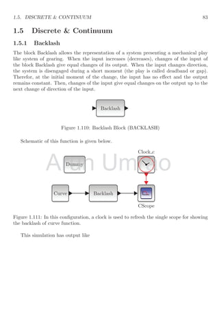
![1.1. SOURCE OF DATA BLOCKS 21
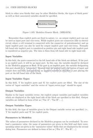
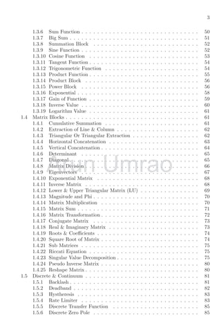
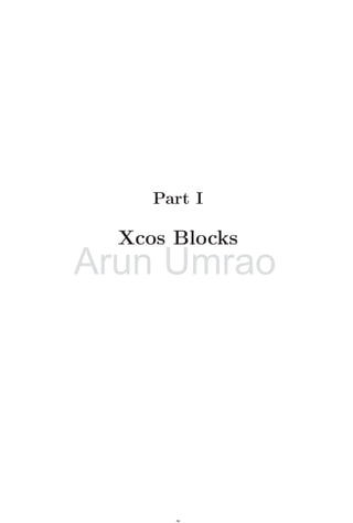
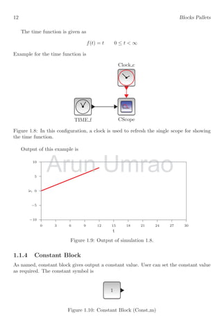
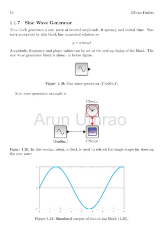
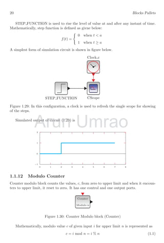
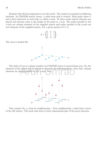
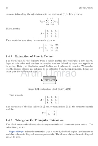
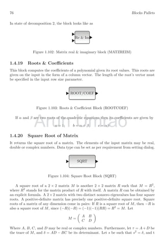
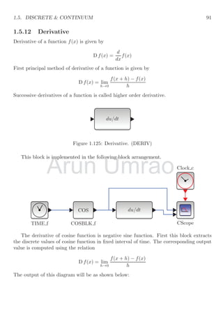
Here, % sign is used to represent modulo in numerical programming. Modulo counter
block simulation is given below
Clock c
CScope
Counter
Modulo 10
Modulo Counter
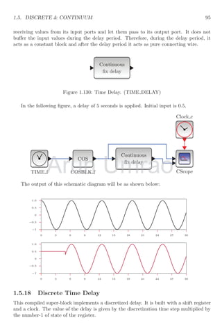
Figure 1.31: In this configuration, a clock is used to refresh the single scope for showing
the counter modulo 10.
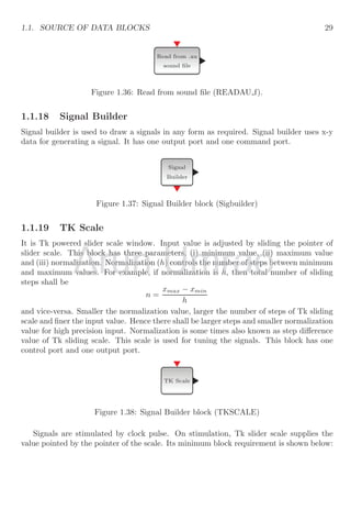
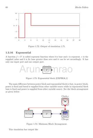
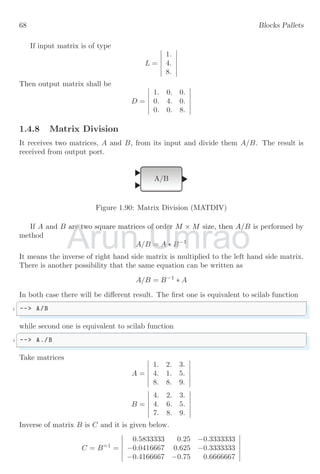
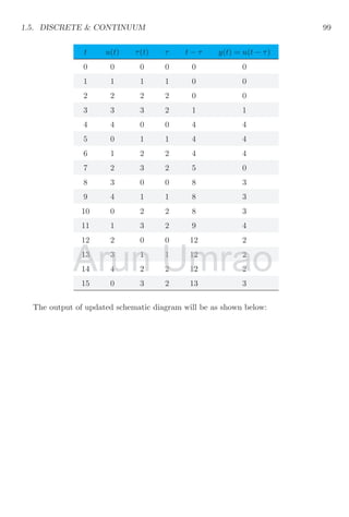
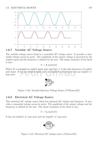
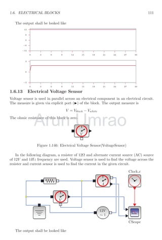
1.1.13 Ramp
Ramp block provide output values according to the relation
y = mt + c
Where y is value provided by ramp at any instant of time t. m, t c are ramp parameters.
m is slope of ramp that determines how fast the output values varies. t is time function
that increases continuously from its initial value. c is initial value of ramp output. Ramp
has only one output port. Derivating to ramp relation
m =
dy
dt
The right side of above relation represent to velocity parameter, therefore, ramp function
also represents to velocity function. The symbol of ramp function is
Figure 1.32: Ramp block (Ramp)
1.1.14 Random Generator
Random generator block generates random values within the two given ranges. The
random value generated by this block is received when clock triggers the block. It has
one control port and one output port. Mathematically
r = R(t)
where, r is sampled random value and R(t) is random value generated by the random
block at time t. The random value r has range a ≤ r ≤ b, i.e. within domain of [a, b].
Arun
is value provided by ramp at any instant of time
is value provided by ramp at any instant of time
is slope of ramp that determines how fast the output values varies.
is slope of ramp that determines how fast the output values varies.
Umrao
mt +
+ c
is value provided by ramp at any instant of time
is value provided by ramp at any instant of time t.
. m,
, t
t
c
c are ramp parameters.
are ramp parameters.
is slope of ramp that determines how fast the output values varies.
is slope of ramp that determines how fast the output values varies. t
t](https://image.slidesharecdn.com/xcossimulation-220117060958/85/Xcos-simulation-21-320.jpg)
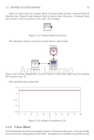
![1.1. SOURCE OF DATA BLOCKS 23
then ith
element of the read record is assumed to be the date of the output event,
i.e. this record is treated as value of t-axis (time variable).
2. Outputs record selection : It is a vector of positive integers like [1, 2, 5]. If read data
is like a vector [k1, k2, . . . kn] then kth
i elements of the read records, i.e. the vector
made of elements [k1, k2, k5] is given in output.
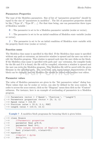
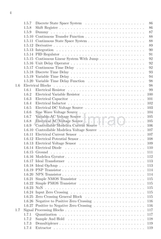
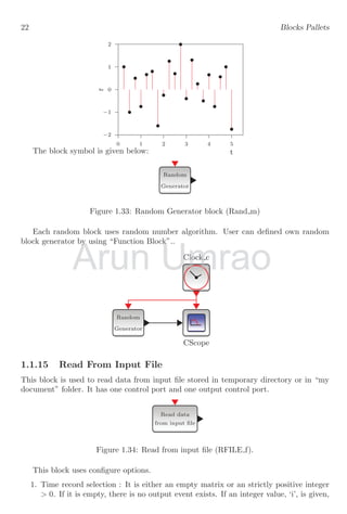
3. Input file name is a file name or path file name. Its value is string of characters.
4. Buffer size : It is similar to the number of bytes read by fread function of C language.
To improve efficiency of input read, file is only done after each Buffer size call to
the block.
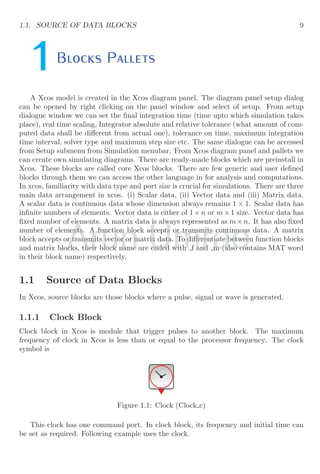
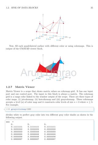
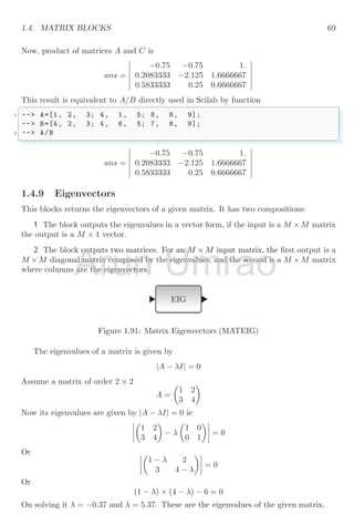
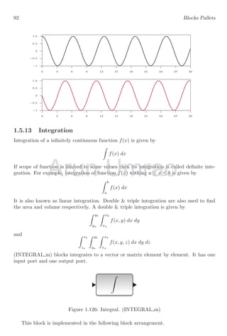
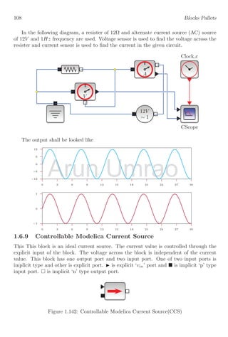
For example, consider a data file myfle.txt with following data except label row
Arun Umrao](https://image.slidesharecdn.com/xcossimulation-220117060958/85/Xcos-simulation-23-320.jpg)
![24 Blocks Pallets
C1 C2 C3
01 0.100 -0.100
02 0.199 -0.199
03 0.296 -0.296
04 0.389 -0.389
05 0.479 -0.479
06 0.565 -0.565
07 0.644 -0.644
08 0.717 -0.717
09 0.783 -0.783
10 0.841 -0.841
11 0.891 -0.891
12 0.932 -0.932
13 0.964 -0.964
14 0.985 -0.985
15 0.997 -0.997
16 1.000 -1.000
17 0.992 -0.992
18 0.974 -0.974
19 0.946 -0.946
20 0.909 -0.909
21 0.863 -0.863
22 0.808 -0.808
23 0.746 -0.746
24 0.675 -0.675
25 0.598 -0.598
26 0.516 -0.516
27 0.427 -0.427
28 0.335 -0.335
29 0.239 -0.239
30 0.141 -0.141
31 0.042 -0.042
32 -0.058 0.058
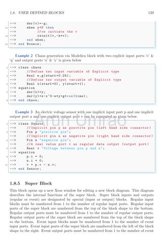
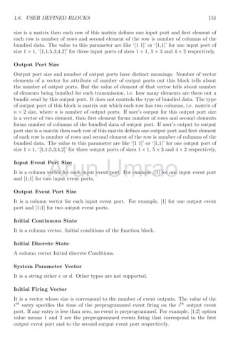
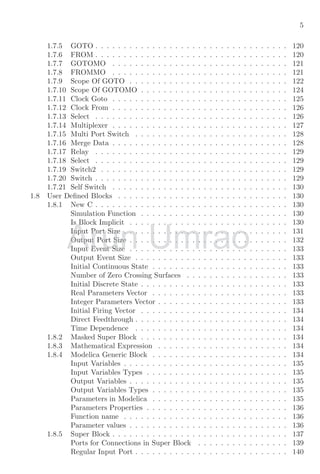
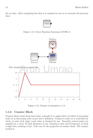
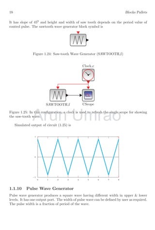
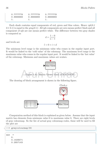
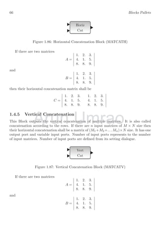
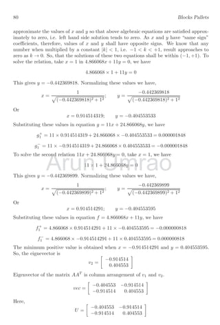
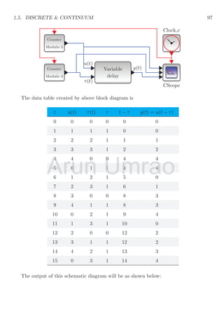
Each row has data record for different entity. Hence the unique data vector for each
row is [k1, k2, k3]. If time record selection is 1, then first column will be used at t values,
i.e. time event values. If this option has value 2, then second column is used at time even
values. Note that, time value is always 0 and continuous increasing, hence block stops
reading of data when either time becomes negative or time starts decreasing. So, time
Arun
16 1.000 -1.000
17
1
18 0.974 -0.974
8 0.974 -0.974
Umrao
6 1.000 -1.000
6 1.000 -1.000
0. -0.992
8 0.974 -0.974
8 0.974 -0.974](https://image.slidesharecdn.com/xcossimulation-220117060958/85/Xcos-simulation-24-320.jpg)
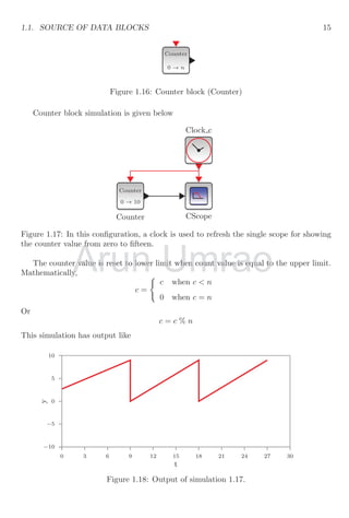
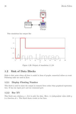
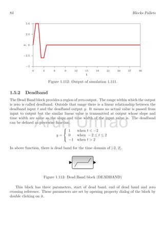
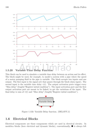
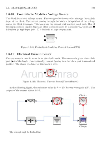
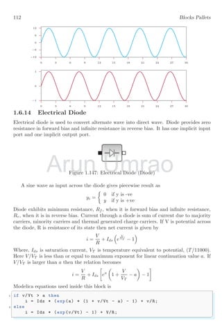
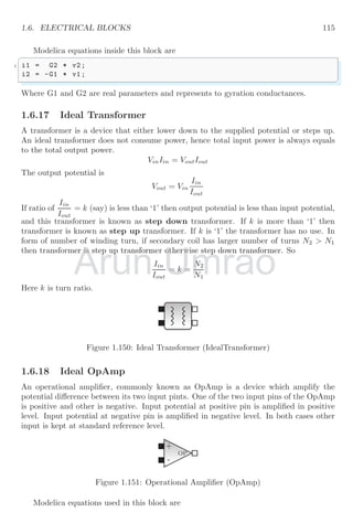
![1.1. SOURCE OF DATA BLOCKS 25
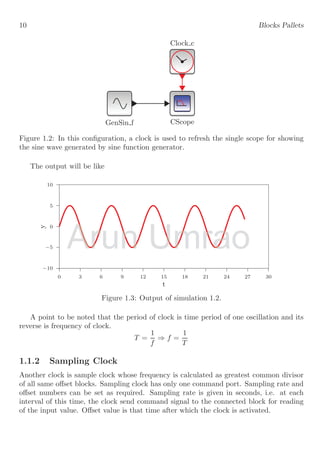
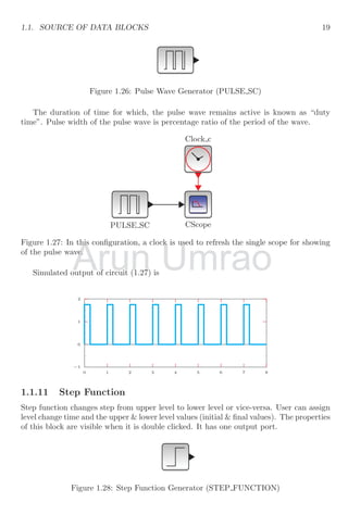
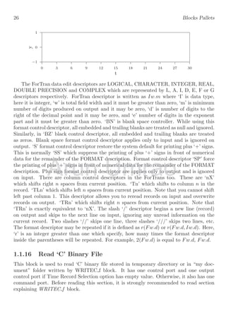
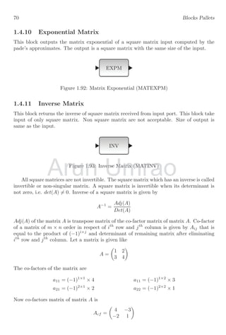
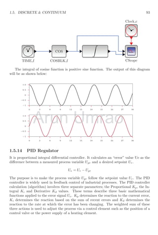
column should be positive, greater than zero and continuous increasing. There are three
output records. If output record selection has value 1 then only data of first column is
sent as output of this block. If the output record selection has value [123] then values in
first, second and third columns will be sent as output of this block.
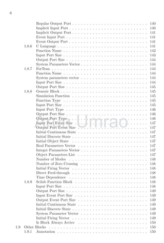
Clock c
CScope
Read data
from input file
RFILE f
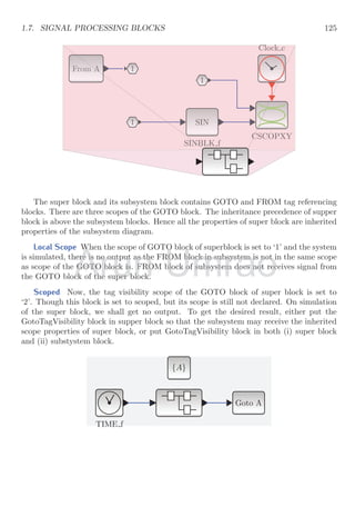
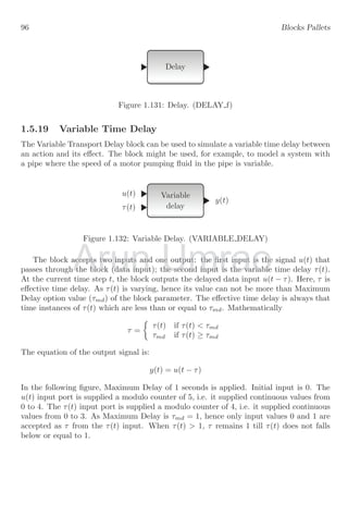
The time record selection is 1 and output record selection is [2, 3]. The output will be
as
−1
0
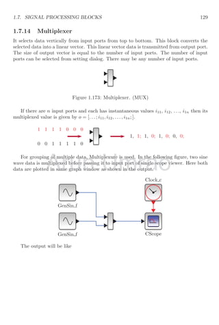
1
0 3 6 9 12 15 18 21 24 27 30
y
t
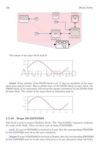
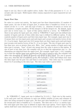
If the time record selection is 2 and output record selection is [2, 3], then time for data
read shall be from t = 0 to t = 1 seconds. After than time starts decreasing hence reading
block will stop reading of data from input data file. And the output will be as
−1
0
1
0 3 6 9 12 15 18 21 24 27 30
y
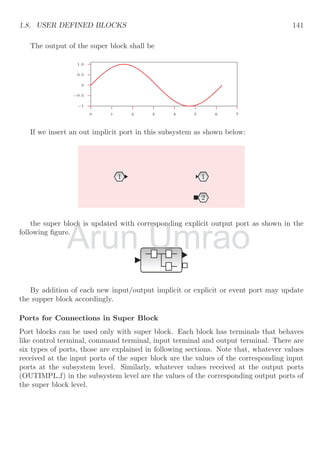
t
If the time record selection is 3 and output record selection is [2, 3], then time for data
read shall be from t = 0 to t = 0 seconds as time value is negative. There will be no
output. Similarly, if time record selection option value is empty, then there is null time,
hence no output.
Arun
Arun
Arun Umrao
Umrao
Umrao](https://image.slidesharecdn.com/xcossimulation-220117060958/85/Xcos-simulation-25-320.jpg)
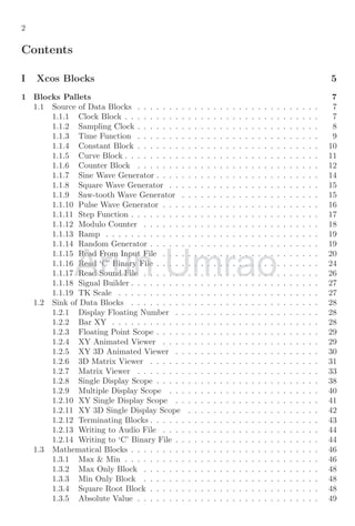
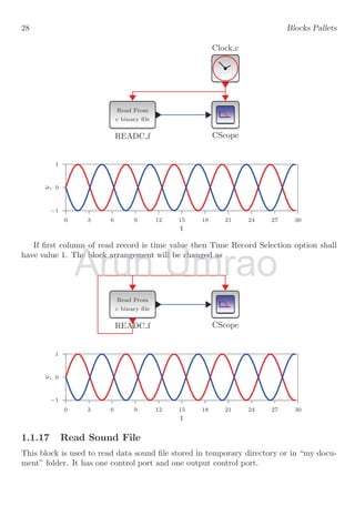
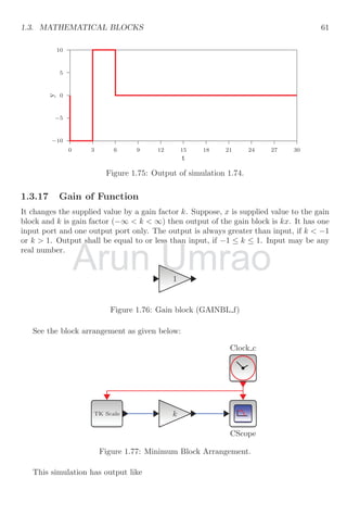
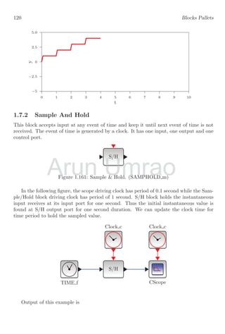
![1.1. SOURCE OF DATA BLOCKS 27
Read from
‘C’ binary file
Figure 1.35: Read from ‘C’ binary file (READC f).
This block uses configure options.
1. Time Record Selection : It is either an empty matrix or an strictly positive integer
greater than zero (scalar). If it is empty, there is no output event port exists. If
an integer value, ‘i’, is given, then ith
element of the read record is assumed to be
the time event value of the output event port, i.e. this record is treated as value of
t-axis (time variable). If this option has value greater than zero, then one command
port is created in this block and ith
will be used as time axis value and also may be
used to control scope viewers.
2. Outputs Record Selection : It is a vector of positive integers like [1, 2, 5]. If read
data is like a vector [k1, k2, . . . kn] then kth
i elements of the read records, i.e. the
vector made of elements [k1, k2, k5] is given in output.
3. Input File Name : It is a file name or path file name. Its value is string of characters.
4. Input Format : A character string defining the data format to use. Strings “l”, “i”,
“s”, “ul”, “ui”, “us”, “d”, “f”, “c”, “uc” are used respectively to write int32, int16,
int8, uint32, uint16, uint8, double, float, char or unsigned char data type. This
value must be same as the value of Output Format option of WRITEC f block.
5. Record Size : This specify the number of columns to be read from C binary file.
This should be same as the input size option of WRITEC f block. If this value is
2 and data being read from C binary file is integer type, then 8 bytes data shall be
read for one record. It is vector of size one.
6. Buffer Size : It is similar to the number of bytes read by fread function of C language.
7. Initial Record Index : This fixes the first record of the file to use. For example, if
record of each entity is arranged in one line and this option is set four, then file will
be read from the fourth line in place of first line.
8. Swap Mode : If Swap mode=1 then file is supposed to be coded in “little endian
IEEE format” and data are swapped if necessary to match the IEEE format of the
processor. If Swap mode=0 then automatic bytes swap is disabled.
A simple block arrangement is shown below:
Arun
4. Input Format : A character string defining the data format to use. Strings “l”, “i”,
4. Input Format : A character string defining the data format to use. Strings “l”, “i”,
“s”, “ul”, “ui”, “us”, “d”, “f”, “c”, “uc” are used respectively to write int32, int16,
“s”, “ul”, “ui”, “us”, “d”, “f”, “c”, “uc” are used respectively to write int32, int16,
int8, uint32, uint16, uint8, double, float, char or unsigned char data type. This
int8, uint32, uint16, uint8, double, float, char or unsigned char data type. This
Umrao
4. Input Format : A character string defining the data format to use. Strings “l”, “i”,
4. Input Format : A character string defining the data format to use. Strings “l”, “i”,
“s”, “ul”, “ui”, “us”, “d”, “f”, “c”, “uc” are used respectively to write int32, int16,
“s”, “ul”, “ui”, “us”, “d”, “f”, “c”, “uc” are used respectively to write int32, int16,
int8, uint32, uint16, uint8, double, float, char or unsigned char data type. This
int8, uint32, uint16, uint8, double, float, char or unsigned char data type. This](https://image.slidesharecdn.com/xcossimulation-220117060958/85/Xcos-simulation-27-320.jpg)
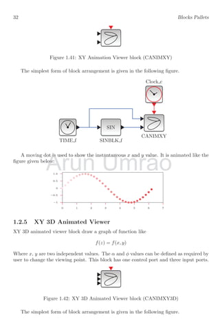
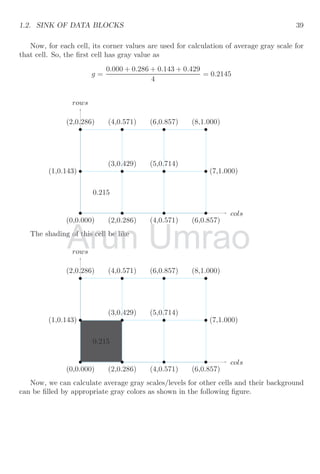
![1.2. SINK OF DATA BLOCKS 31
1.2.3 Floating Point Scope
Floating point scope, shows output of floating points ranges between zero to one. It has
one control port. The output viewed in this scope is
y = (float)x
Figure 1.40: Floating Point Scope (CFSCOPE)
Following parameters of the block can be set as and when required.
Color Set the number for color of output graph.
Output Window Number Output windows are assigned an identification numbers for
processing of data. By default it is ‘-1’. It means the window number will automatically
assigned an ID. Apart from it, user defined ID can also be assigned to the window.
Output Window Position Position of window tell the window that where it will posi-
tioned after opening. By default it is positioned in center of screen. The xy-coordinates
of window position are assigned like [x; y]. The coordinates are calculated from the top
left corner of the screen of computer system.
Output Window Sizes It determines the size of output window. The coordinates are
syntax as [x; y].
Ymin It is the minimum value of the output to be displayed in the output window.
Ymin is used to set the lower scale point of the y-axis in output display.
YMax It is the maximum value of the output to be displayed in the output window.
Ymax is used to set the upper scale point of the y-axis in output display.
Refresh Period It is the maximum range of independent variable to be displayed in
the output window.
Buffer Size The size of output values to be stored in the memory. The drawing is
only done after each Buffer size call to the block.
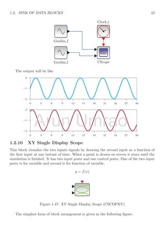
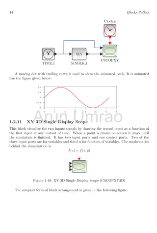
1.2.4 XY Animated Viewer
XY animated viewer visualized the second input with respect first input as a function of
first input at instant simulated time. Mathematically
y = f(x)
The output plot is two dimensional. It has two input ports and one control port. One of
the two input ports is for variable and second is for function of variable.
Arun
Output Window Position
Output Window Position Position of window tell the window that where it will posi-
Position of window tell the window that where it will posi-
ioned after opening. By default it is positioned in center of screen. The xy-coordinates
ioned after opening. By default it is positioned in center of screen. The xy-coordinates
of window position are assigned like [
of window position are assigned like [ Umrao
Position of window tell the window that where it will posi-
Position of window tell the window that where it will posi-
ioned after opening. By default it is positioned in center of screen. The xy-coordinates
ioned after opening. By default it is positioned in center of screen. The xy-coordinates
y]. The coordinates are calculated from the top
]. The coordinates are calculated from the top](https://image.slidesharecdn.com/xcossimulation-220117060958/85/Xcos-simulation-31-320.jpg)
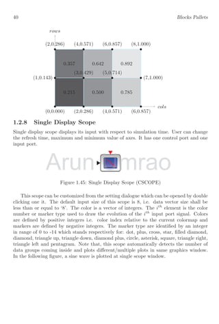
![1.2. SINK OF DATA BLOCKS 37
0.4285714
0.5714286
0.7142857
0.8571429
1.
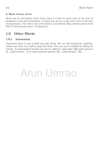
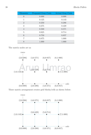
Let the matrix elements are arranged in the xy-plane taking x-axis as rows and y-axis as
columns. The experimental matrix is
1 -- M=[0 1 2; 2 3 4; 4 5 6;6 7 8]
M=
0. 1. 2.
2. 3. 4.
4. 5. 6.
6. 7. 8.
Now, the minimum matrix value (say 0) is set to gray color level 0 and maximum matrix
value (say 8) is set to gray color level 1. The intermediate distinct matrix elements are
assigned proposed gray color code from equally distributed gray colormap values ranging
from 0 to 1 as shown in the below table.
Matrix Element Proposed Gray Code
0 0.000
1 0.125
2 0.250
3 0.375
4 0.500
5 0.625
6 0.750
7 0.875
8 1.000
As there are 8 colormap levels and 9 distinct matrix elements, hence the proposed
gray color codes are rounded to near gray colormap values of actual gray colormap. Thus
the actual table will be
Arun
Matrix Elemen
Umrao
Proposed Gray Code
0.000](https://image.slidesharecdn.com/xcossimulation-220117060958/85/Xcos-simulation-37-320.jpg)
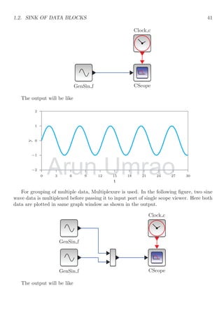
![1.2. SINK OF DATA BLOCKS 47
1. Input Size : It is size of input column vector. A scalar that determines the how
many columns of data values are used to form a record. This description must
be read with the data output format description. Suppose, we have define integer
datatype data format and input size is 2 then total 8 bytes shall be used to write a
record of data in binary form. The data received at input port of WRITEC f block
must be of same size as defined in the Input Size option.
2. Output File Name : It is a file name or path file name where data would be written.
Its value is string of characters.
3. Output Format : A character string defining the data format to use. Strings “l”,
“i”, “s”, “ul”, “ui”, “us”, “d”, “f”, “c”, “uc” are used respectively to write int32,
int16, int8, uint32, uint16, uint8, double, float, char or unsigned char data type.
4. Buffer Size : It is similar to the number of bytes read by fread function of C language.
5. Swap Mode : If swap mode=1 then file is supposed to be coded in “little endian
IEEE format” and data are swapped if necessary to match the IEEE format of the
processor. If Swap mode=0 then automatic bytes swap is disabled.
Clock c
Write to C
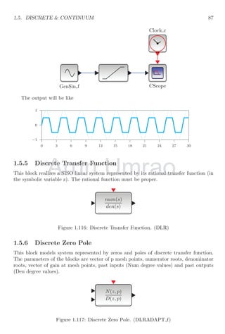
GenSin f
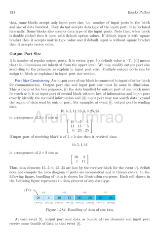
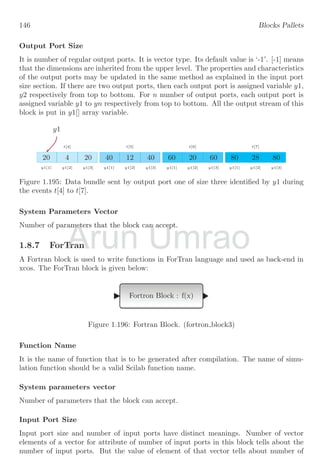
The above block diagram is indicative purpose about the use of WRITEC f. The data
written by this block is in format as shown below:
rec[4]
20 4
byte[1] byte[2]
rec[5]
40 12
byte[1] byte[2]
rec[6]
60 20
byte[1] byte[2]
rec[7]
80 28
byte[1] byte[2]
wr
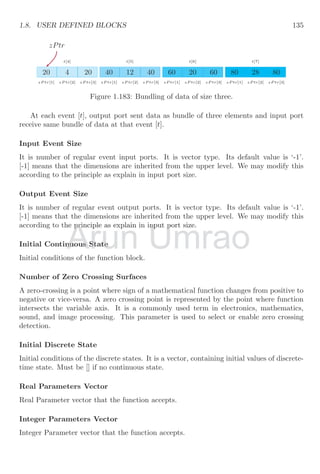
In this figure, we have explained that the character type data with size two is saved in
binary format. First byte is for one of the two data elements of a record and second byte
is for other of the two data elements of a record. The number of bytes required depends
on the type of data and size of data. A character data type requires one byte memory
space and if record size is two then two bytes are required to save a record. If data type
is integer type and data size is two, then memory arrangement shall be like
rec[4]
0 0 20 4
byte[1] byte[2] byte[3] byte[4]
rec[5]
0 0 40 12
byte[1] byte[2] byte[3] byte[4]
rec[6]
0 0 60 20
byte[1] byte[2] byte[3] byte[4]
wr
Arun Umrao
Umrao
Umrao
Umrao
Umrao
Umrao
Umrao
Umrao
Umrao
Umrao
Umrao
Umrao
Umrao
Umrao
Umrao
Umrao
Umrao
Umrao
Umrao
Umrao
Umrao
Umrao
Umrao
Umrao
Umrao
Umrao
Umrao
Umrao
Umrao
Umrao
Umrao
Umrao
Umrao
Umrao
Umrao
Umrao
Umrao
Umrao
Umrao
Umrao
Umrao
Umrao
Umrao
Umrao
Umrao
Umrao
Umrao
Umrao
Umrao
Umrao
Umrao
Umrao
Umrao
Umrao
Umrao
Umrao
Umrao
Umrao
Umrao
Umrao
Umrao
Umrao
Umrao
Umrao
Umrao
Umrao
Umrao
Umrao
Umrao
Umrao
Umrao
Umrao
Umrao
Umrao
Umrao
Umrao
Umrao
Umrao
Umrao
Umrao
Umrao
Umrao
Umrao
Umrao
Umrao
Umrao
Umrao
Umrao
Umrao
Umrao
Umrao
Umrao
Umrao
Umrao
Umrao
Umrao
Umrao
Umrao
Umrao
Umrao
Umrao
Umrao
Umrao
Umrao
Umrao
Umrao
Umrao
Umrao
Umrao
Umrao
Umrao
Umrao
Umrao
Umrao
Umrao
Umrao
Umrao
Umrao
Umrao
Umrao
Umrao
Umrao
Umrao
Umrao
Umrao
Umrao
Umrao
Umrao
Umrao
Umrao
Umrao
Umrao
Umrao
Umrao
Umrao
Umrao
Umrao
Umrao
Umrao
Umrao
Umrao
Umrao
Umrao
Umrao
Umrao
Umrao
Umrao
Umrao
Umrao
Umrao
Umrao
Umrao
Umrao
Umrao
Umrao
Umrao
Umrao
Umrao
Umrao
Umrao
Umrao
Umrao
Umrao
Umrao
Umrao
Umrao
Umrao
Umrao
Umrao
Umrao
Umrao
Umrao
Umrao
Umrao
Umrao
Umrao
Umrao
Umrao
Umrao
Umrao
Umrao
Umrao
Umrao
Umrao
Umrao
Umrao
Umrao
Umrao
Umrao
Umrao
Umrao
Umrao
Umrao
Umrao
Umrao
Umrao
Umrao
Umrao
Umrao
Umrao
Umrao
Umrao
Umrao
Umrao
Umrao
Umrao
Umrao
Umrao
Umrao
Umrao
Umrao
Umrao
Umrao
Umrao
Umrao
Umrao
Umrao
Umrao
Umrao
Umrao
Umrao
Umrao
Umrao
Umrao
Umrao
Umrao
Umrao
Umrao
Umrao
Umrao
Umrao
Umrao
Umrao
Umrao
Umrao
Umrao
Umrao
Umrao
Umrao
Umrao
Umrao
Umrao
Umrao
Umrao
Umrao
Umrao
Umrao
Umrao
Umrao
Umrao
Umrao
Umrao
Umrao
Umrao
Umrao
Umrao
Umrao
Umrao
Umrao
Umrao
Umrao
Umrao
Umrao
Umrao
Umrao
Umrao
Umrao
Umrao
Umrao
Umrao
Umrao
Umrao
Umrao
Umrao
Umrao
Umrao
Umrao
Umrao
Umrao
Umrao
Umrao
Umrao
Umrao
Umrao
Umrao
Umrao
Umrao
Umrao
Umrao
Umrao
Umrao
Umrao
Umrao
Umrao
Umrao
Umrao
Umrao
Umrao
Umrao
Umrao
Umrao
Umrao
Umrao
Umrao
Umrao
Umrao
Umrao
Umrao
Umrao
Umrao
Umrao
Umrao
Umrao
Umrao
Umrao
Umrao
Umrao
Umrao
Umrao
Umrao
Umrao
Umrao
Umrao
Umrao
Umrao
Umrao
Umrao
Umrao
Umrao
Umrao
Umrao
Umrao
Umrao
Umrao
Umrao
Umrao
Umrao
Umrao
Umrao
Umrao
Umrao
Umrao
Umrao
Umrao
Umrao
Umrao
Umrao
Umrao
Umrao
Umrao
Umrao
Umrao
Umrao
Umrao
Umrao
Umrao
Umrao
Umrao
Umrao
Umrao](https://image.slidesharecdn.com/xcossimulation-220117060958/85/Xcos-simulation-47-320.jpg)
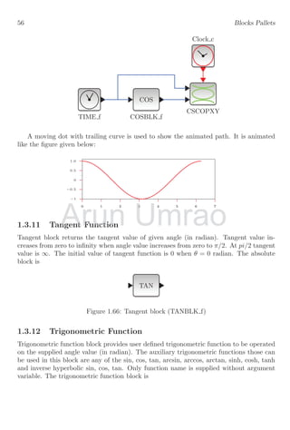
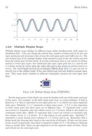
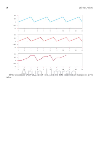
![1.3. MATHEMATICAL BLOCKS 53
−1
−0.5
0
0.5
1.0
0 3 6 9 12 15 18 21 24 27 30
−1
−0.5
0
0.5
1.0
0 3 6 9 12 15 18 21 24 27 30
−2
−1.5
−1.0
−0.5
0
0.5
1.0
1.5
2.0
0 3 6 9 12 15 18 21 24 27 30
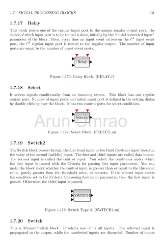
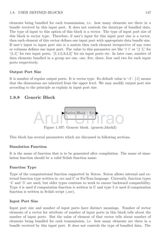
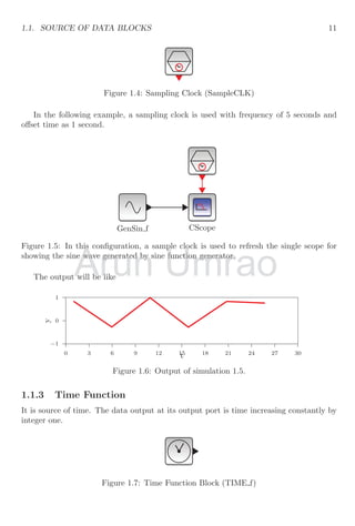
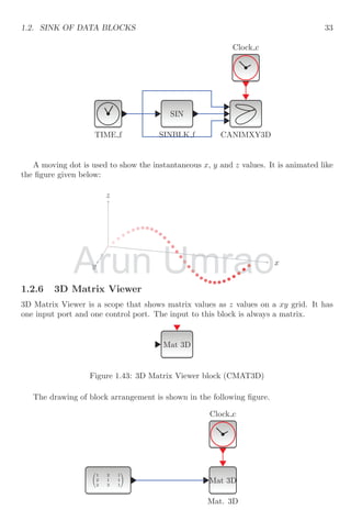
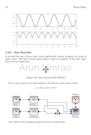
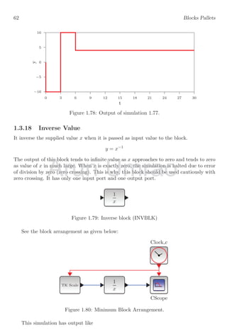
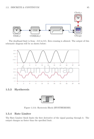
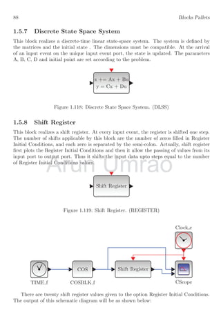
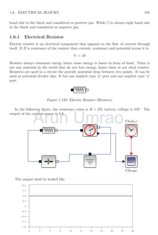
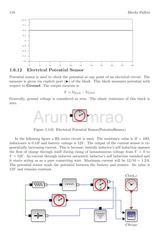
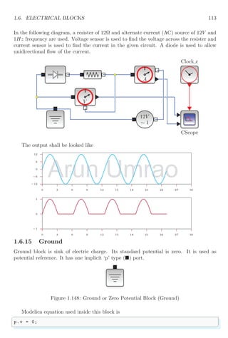
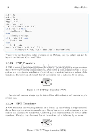
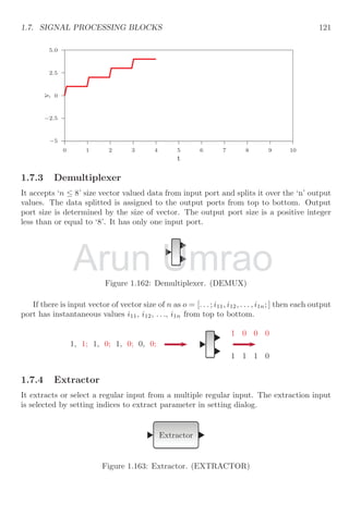
1.3.7 Big Sum
It provides the sum of two or more real input values algebraically either by accepting
them as they are or by changing their nature. User can change the number of input. It
has unlimited input ports and one output port. Number of input ports depends on the
input port matrix. Each element in port matrix represents one input port. The numerical
value of each element is the gain of input values. Gain of input port ranges from 0 to
∞. For example [0; 1; −2] represents to the three input ports and first port has zero gain,
second port has +1 gain and third port has −2 gain1
.
X
Figure 1.61: Big sum block (BIGSOM f)
The additive or subtractive nature of input port can be assigned by using plus or minus
sign in port matrix. If both signs are assigned to the input ports then their additive or
subtractive nature of input ports are shown by plus or minus sign.
1
Gain is defined as the ratio of final value to the initial value
Arun
Arun Umrao
Umrao](https://image.slidesharecdn.com/xcossimulation-220117060958/85/Xcos-simulation-77-320.jpg)
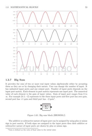
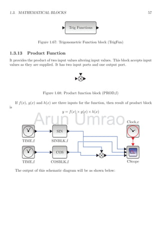
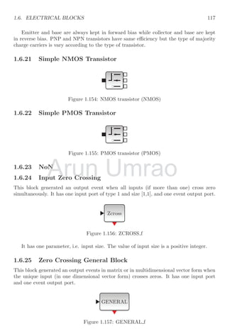
![54 Blocks Pallets
+
-
X
Figure 1.62: Big sum block (BIGSOM f)
If α, β and γ are three gains of the three inputs of the big sum and their input values
are i, j and k respectively, then the result output of this function shall be algebraic sum
of the product input port gain and their corresponding inputs.
y = αi + βj + γj
This is obsolete block.
1.3.8 Summation Block
It provides the sum of two or more input vector values algebraically. User can change the
number of input ports. It unlimited input ports and one output port. Input ports can
be assigned only either +1 or −1 values i.e. [1; −1; 1; 1; 1] etc. The gain of input values
is only 1 in factor.
+
-
X
Figure 1.63: Summation block (SUMMATION)
The principal difference between big sum block and summation block is that summa-
tion block can add two or more real or imaginary or complex or int32 values. It also give
warning or do nothing or shows saturated values when data overflows.
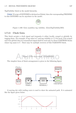
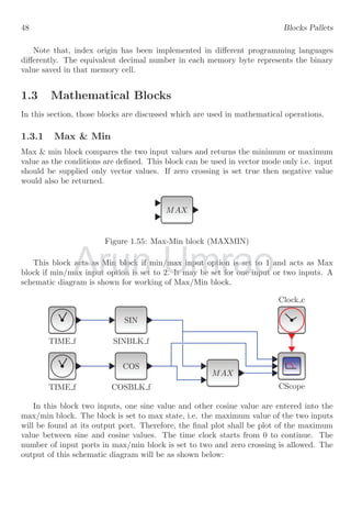
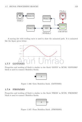
1.3.9 Sine Function
Sine block returns the sine value of given angle (in radian). The maximum and minimum
value of sine function lies between ±1. The initial value of sine function is 0 when θ = 0
radian. The sine block is
SIN
Figure 1.64: Sine block (SINBLK f)
The simplest form of block arrangement is given in the following figure.
Arun Umrao
Umrao
Umrao
Umrao
Umrao
Umrao
Umrao
Umrao
Umrao
Umrao
Umrao
Umrao
Umrao
Umrao
Umrao
Umrao
Umrao
Umrao
Umrao
Umrao
Umrao
Umrao
Umrao
Umrao
Umrao
Umrao
Umrao
Umrao
Umrao
Umrao
Umrao
Umrao
Umrao
Umrao
Umrao
Umrao
Umrao
Umrao
Umrao
Umrao
Umrao
Umrao
Umrao
Umrao
Umrao
Umrao
Umrao
Umrao
Umrao
Umrao
Umrao
Umrao
Umrao
Umrao
Umrao
Umrao
Umrao
Umrao
Umrao
Umrao
Umrao
Umrao
Umrao
Umrao
Umrao
Umrao
Umrao
Umrao
Umrao
Umrao
Umrao
Umrao
Umrao
Umrao
Umrao
Umrao
Umrao
Umrao
Umrao
Umrao
Umrao
Umrao
Umrao
Umrao
Umrao
Umrao
Umrao
Umrao
Umrao
Umrao
Umrao
Umrao
Umrao
Umrao
Umrao
Umrao
Umrao
Umrao
Umrao
Umrao
Umrao
Umrao
Umrao
Umrao
Umrao
Umrao
Umrao
Umrao
Umrao
Umrao
Umrao
Umrao
Umrao
Umrao
Umrao
Umrao
Umrao
Umrao
Umrao
Umrao
Umrao
Umrao
Umrao
Umrao
Umrao
Umrao
Umrao
Umrao
Umrao
Umrao
Umrao
Umrao
Umrao
Umrao
Umrao
Umrao
Umrao
Umrao
Umrao
Umrao
Umrao
Umrao
Umrao
Umrao
Umrao
Umrao
Umrao
Umrao
Umrao
Umrao
Umrao
Umrao
Umrao
Umrao
Umrao
Umrao
Umrao
Umrao
Umrao
Umrao
Umrao
Umrao
Umrao
Umrao
Umrao
Umrao
Umrao
Umrao
Umrao
Umrao
Umrao
Umrao
Umrao
Umrao
Umrao
Umrao
Umrao
Umrao
Umrao
Umrao
Umrao
Umrao
Umrao
Umrao
Umrao
Umrao
Umrao
Umrao
Umrao
Umrao
Umrao
Umrao
Umrao
Umrao
Umrao
Umrao
Umrao
Umrao
Umrao
Umrao
Umrao
Umrao
Umrao
Umrao
Umrao
Umrao
Umrao
Umrao
Umrao
Umrao
Umrao
Umrao
Umrao
Umrao
Umrao
Umrao
Umrao
Umrao
Umrao
Umrao
Umrao
Umrao
Umrao
Umrao
Umrao
Umrao
Umrao
Umrao
Umrao
Umrao
Umrao
Umrao
Umrao
Umrao
Umrao
Umrao
+
+
+
+
+
+
+
+
+
+
+
+
+
+
+
+
+
+
+
+
+
+
+
+
+
+
+
+
+
+
+
+
+
+
+
+
+
+
Umrao
X
X
X
X
X
X
X
X
X
X
X
X
X
X
X
X
X
X
X
X
X
X
X
X
X
X
X
X
X
X
X
X
X
X
X
X
X
X
X
X
X
X
X
X
X
X
X
X
X
X
X
X
X
X
X
X
X
X](https://image.slidesharecdn.com/xcossimulation-220117060958/85/Xcos-simulation-78-320.jpg)
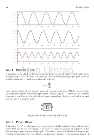
![58 Blocks Pallets
−1
−0.5
0
0.5
1.0
0 3 6 9 12 15 18 21 24 27 30
−1
−0.5
0
0.5
1.0
0 3 6 9 12 15 18 21 24 27 30
−1
−0.5
0
0.5
1.0
0 3 6 9 12 15 18 21 24 27 30
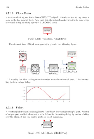
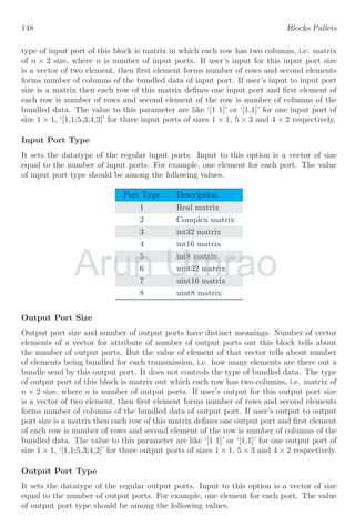
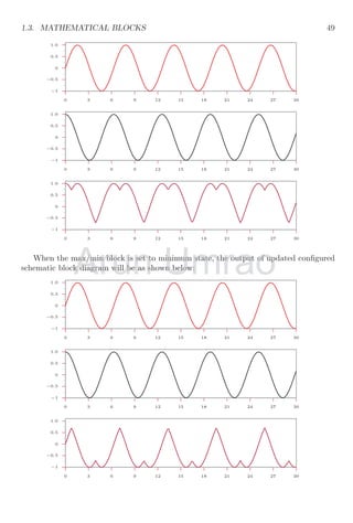
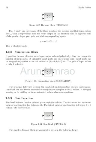
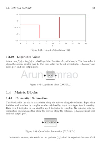
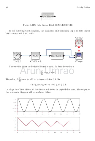
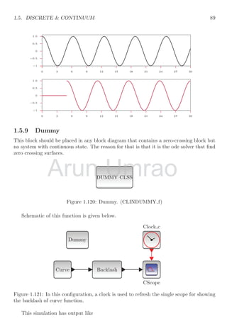
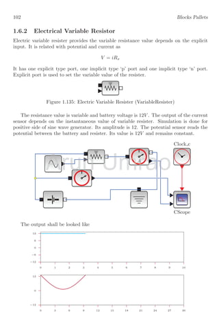
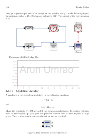
1.3.14 Product Block
It provides the product or division of two or more real input values. Each port can be
assigned only +1 or −1 value. +1 indicates that the corresponding input port performs
multiplication and −1 performs division in order of
y =
Q
i
Q
j
Here i represents to all the number inputs at product input ports. While j represents to
all the number inputs at division input ports. Port data [1; 1; −1] represents to the three
input ports and first port is multiplicative port, second port is also a multiplicative port
and third port is divisive port.
Y
Figure 1.69: Product block (PRODUCT)
1.3.15 Power Block
A function f = ua
is called power of u to a times. u is the supplied value and a is fixed
power that can be set accordingly. The value of a may be positive or negative. It has
only one input port and one output port. Note that, there shall be error if there is zero
crossing for negative power or output is an imaginary number. The reason is than
√
−2
Arun
1.3.14 Product Block
1.3.14 Product Block
t provides the product or division of two or more real input values. Each port can be
t provides the product or division of two or more real input values. Each port can be
Umrao
t provides the product or division of two or more real input values. Each port can be
t provides the product or division of two or more real input values. Each port can be](https://image.slidesharecdn.com/xcossimulation-220117060958/85/Xcos-simulation-82-320.jpg)
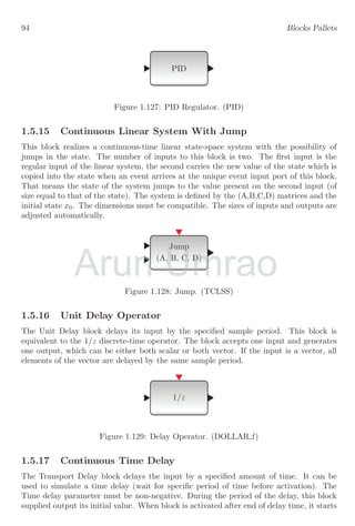
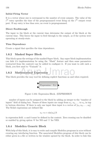
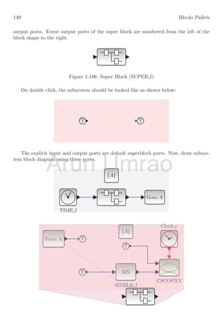
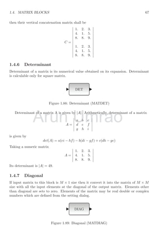
![The extraction of the line indices [1 2] and column indices [1 2], the extracted matrix
shall be
B =](https://image.slidesharecdn.com/xcossimulation-220117060958/85/Xcos-simulation-124-320.jpg)