boundary layer aerodynamics

1. 1
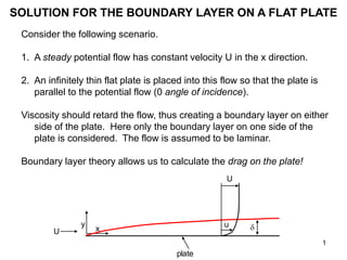
SOLUTION FOR THE BOUNDARY LAYER ON A FLAT PLATE
Consider the following scenario.
1. A steady potential flow has constant velocity U in the x direction.
2. An infinitely thin flat plate is placed into this flow so that the plate is
parallel to the potential flow (0 angle of incidence).
Viscosity should retard the flow, thus creating a boundary layer on either
side of the plate. Here only the boundary layer on one side of the
plate is considered. The flow is assumed to be laminar.
Boundary layer theory allows us to calculate the drag on the plate!
x
y d
U
U
u
plate

2. 2
A STEADY RECTILINEAR POTENTIAL FLOW HAS ZERO
PRESSURE GRADIENT EVERYWHERE
x
y d
U
U
u
plate
A steady, rectilinear potential flow in the x direction is described by the
relations
According to Bernoulli’s equation for potential flows, the dynamic
pressure of the potential flow ppd is related to the velocity field as
Between the above two equations, then, for this flow
0
y
v
,
U
x
u
,
Ux 











const
)
v
u
(
2
1
p 2
2
pd 



0
y
p
x
p pd
pd







3. 3
BOUNDARY LAYER EQUATIONS FOR A FLAT PLATE
x
y d
U
U
u
plate
For the case of a steady, laminar boundary layer on a flat plate at 0
angle of incidence, with vanishing imposed pressure gradient, the
boundary layer equations and boundary conditions become (see Slide
15 of BoundaryLayerApprox.ppt with dppds/dx = 0)
0
y
v
x
u
y
u
y
u
v
x
u
u 2
2















U
u
,
0
v
,
0
u y
0
y
0
y


 



Tangential and normal velocities
vanish at boundary: tangential
velocity = free stream velocity far
from plate
0
y
v
x
u
y
u
dx
dp
1
y
u
v
x
u
u 2
2
pds



















4. 4
NOMINAL BOUNDARY LAYER THICKNESS
x
y d
U
U
u
plate
Until now we have not given a precise definition for boundary layer
thickness. Here we use d to denote nominal boundary thickness, which
is defined to be the value of y at which u = 0.99 U, i.e.
U
99
.
0
)
y
,
x
(
u y

d

x
y
u
U
u = 0.99 U
d
The choice 0.99 is arbitrary; we could have chosen 0.98 or 0.995 or
whatever we find reasonable.

5. 5
STREAMWISE VARIATION OF BOUNDARY LAYER
THICKNESS
Consider a plate of length L. Based on the estimate of Slide 11 of
BoundaryLayerApprox.ppt, we can estimate d as
or thus
where C is a constant. By the same arguments, the nominal boundary
thickness up to any point x  L on the plate should be given as


d  UL
,
)
(
~
L
2
/
1
Re
Re
2
/
1
2
/
1
U
L
C
or
U
L
~ 




 

d





 
d
2
/
1
2
/
1
U
x
C
or
U
x
~ 




 

d





 
d
x
y d
U
U
u
plate
L

6. 6
SIMILARITY
One triangle is similar to another triangle if it can be mapped onto the
other triangle by means of a uniform stretching.
The red triangles are similar
to the blue triangle.
The red triangles are not
similar to the blue triangle.
Perhaps the same idea can be applied to the solution of our problem:
0
y
v
x
u
,
y
u
y
u
v
x
u
u 2
2















U
u
,
0
v
,
0
u y
0
y
0
y


 




7. 7
SIMILARITY SOLUTION
Suppose the solution has the property that when u/U is plotted against y/d
(where d(x) is the previously-defined nominal boundary layer thickness) a
universal function is obtained, with no further dependence on x. Such a
solution is called a similarity solution. To see why, consider the sketches
below. Note that by definition u/U = 0 at y/d = 0 and u/U = 0.99 at y/d = 1,
no matter what the value of x. Similarity is satisfied if a plot of u/U versus
y/d defines exactly the same function regardless of the value of x.
plate
x
y d
U
U
u
u
U
x1 x2
0
0
1
1
u/U
y/d
profiles at
x1 and x2
0
0
1
1
u/U
y/d
profile at x1
profile at x2
Similarity
satisfied
Similarity not
satisfied

8. 8
SIMILARITY SOLUTION contd.
So for a solution obeying similarity in the velocity profile we must have
where g1 is a universal function, independent of x (position along the
plate). Since we have reason to believe that
where C is a constant (Slide 5), we can rewrite any such similarity form as
Note that  is a dimensionless variable.
If you are wondering about the constant C, note the following. If y is a
function of x alone, e.g. y = f1(x) = x2 + ex, then y is a function of p = 3x
alone, i.e. y = f(p) = (p/3)2 + e(p/3).






d

)
x
(
y
f
U
u
1
2
/
1
2
/
1
U
x
C
or
U
x
~ 




 

d





 
d
x
U
y
U
x
y
,
)
(
f
U
u
2
/
1







 





9. 9
BUT DOES THE PROBLEM ADMIT A SIMILARITY
SOLUTION?
Maybe, maybe not, you never know until you try. The problem is:
This problem can be reduced with the streamfunction (u = /y, v = -
/x) to:
Note that the stream function satisfies continuity identically. We are not
using a potential function here because boundary layer flows are not
potential flows.
0
y
v
x
u
,
y
u
y
u
v
x
u
u 2
2















U
u
,
0
v
,
0
u y
0
y
0
y


 



3
3
2
y
y
x
y
x
y 


















U
y
,
0
x
,
0
y y
0
y
0
y

















10. 10
SOLUTION BY THE METHOD OF GUESSING
We want our streamfunction to give us a velocity u = /y satisfying the
similarity form
So we could start off by guessing
where f is another similarity function.
But this does not work. Using the prime to denote ordinary differentiation
with respect to , if  = f() then
But
x
U
y
,
)
(
f
U
u





)
(
F 


y
)
(
F
y
u










x
U
y 




so that )
(
F
x
U
1
U
u





11. 11
SOLUTION BY THE METHOD OF GUESSING contd.
So if we assume
then we obtain
This form does not satisfy the condition that u/U should be a function of 
alone. If F is a function of  alone then its first derivative F’() is also a
function of  alone, but note the extra (and unwanted) functionality in x via
the term (Ux)-1/2!
So our first try failed because of the term (Ux)-1/2.
Let’s not give up! Instead, let’s learn from our mistakes!
)
(
F 


)
(
F
x
U
1
U
u




not OK OK

12. 12
ANOTHER TRY
This time we assume
Now remembering that x and y are independent of each other and
recalling the evaluation of /y of Slide 10,
or thus
Thus we have found a form of  that satisfies similarity in velocity!
But this does not mean that we are done. We have to solve for the
function F().
)
(
F
x
U 



)
(
F
U
x
U
)
(
F
x
U
y
)
(
F
x
U
y
u 


















)
(
F
)
(
f
,
)
(
f
U
u







13. 13
REDUCTION FROM PARTIAL TO ORDINARY
DIFFERENTIAL EQUATION
Our goal is to reduce the partial differential equation for and boundary
conditions on , i.e.
to an ordinary differential equation for and boundary conditions on f(),
where
To do this we will need the following forms:
3
3
2
y
y
x
y
x
y 


















U
y
,
0
x
,
0
y y
0
y
0
y
















x
U
y
,
)
(
F
x
U







x
U
y 




x
2
1
x
U
y
2
1
x
2
/
3 







 

14. 14
The next steps involve a lot of hard number crunching. To evaluate the
terms in the equation below,
we need to know /y, 2/y2, 3/y3, /x and 2/yx, where
Now we have already worked out /y; from Slide 12:
Thus
REDUCTION contd.
3
3
2
y
y
x
y
x
y 


















x
U
y
,
)
(
F
x
U







x
2
1
x
,
x
U
y











)
(
F
x
U
U
y
)
(
F
U
y2
2















)
(
F
U
y






)
(
F
x
U
U
y
)
(
F
x
U
U
y3
3



















15. 15
Again using
we now work out the two remaining derivatives:
REDUCTION contd.
x
U
y
,
)
(
F
x
U







x
2
1
x
,
x
U
y











 
)
(
F
)
(
F
x
U
2
1
x
)
(
F
x
U
)
(
F
x
U
2
1
)
(
F
x
U
x
x

























 
  )
y
(
F
x
U
2
1
y
)
(
F
)
(
F
)
(
F
x
U
2
1
)
(
F
)
(
F
x
U
2
1
y
x
y
y
x
2


























































16. 16
Summarizing,
REDUCTION contd.
x
U
y
,
)
(
F
x
U







x
2
1
x
,
x
U
y











 
)
(
F
)
(
F
x
U
2
1
x










)
y
(
F
x
U
2
1
y
x
2









)
(
F
U
y






)
(
F
x
U
U
y2
2








)
(
F
x
U
U
y3
3










17. 17
Now substituting
into
yields
or thus
Similarity works! It has cleaned up the mess into a simple (albeit
nonlinear) ordinary differential equation!
REDUCTION contd.
 
)
(
F
)
(
F
x
U
2
1
x











)
y
(
F
x
U
2
1
y
x
2









)
(
F
U
y






)
(
F
x
U
U
y2
2







 )
(
F
x
U
U
y3
3









3
3
2
y
y
x
y
x
y 


















F
x
U
F
)
F
F
(
x
U
2
1
F
F
x
U
2
1 2
2
2















0
F
F
F
2 







18. 18
From Slide 9, the boundary conditions are
But we already showed that
Now noting that  = 0 when y = 0, the boundary conditions reduce to
Thus we have three boundary conditions for the 3rd-order differential
equation
BOUNDARY CONDITIONS
 
)
(
F
)
(
F
x
U
2
1
x










)
(
F
U
y






0
F
F
F
2 






U
y
,
0
x
,
0
y y
0
y
0
y
















x
U
y



1
)
(
F
,
0
)
0
(
F
,
0
)
0
(
F 






19. 19
There are a number of ways in which the problem
can be solved. It is beyond the scope of this course to illustrate numerical
methods for doing this. A plot of the solution is given below.
SOLUTION
0
F
F
F
2 





 1
)
(
F
,
0
)
0
(
F
,
0
)
0
(
F 





Blasius Solution, Laminar Boundary Layer
0
1
2
3
4
5
6
0 0.5 1 1.5 2 2.5 3 3.5 4 4.5
f, f', f''

f()
f'()
f''() F
F
F 

F
,
F
,
F 



20. 20
To access the numbers, double-click on the Excel spreadsheet below.
Recall that
SOLUTION contd.
 F F' F''
0 0 0 0.33206
0.1 0.00166 0.033206 0.332051
0.2 0.006641 0.066408 0.331987
0.3 0.014942 0.099599 0.331812
0.4 0.02656 0.132765 0.331473
0.5 0.041493 0.165887 0.330914
0.6 0.059735 0.198939 0.330082
0.7 0.081278 0.231892 0.328925
0.8 0.106109 0.264711 0.327392
0.9 0.134214 0.297356 0.325435
1 0.165573 0.329783 0.32301
1.1 0.200162 0.361941 0.320074
1.2 0.237951 0.393779 0.316592
1.3 0.278905 0.42524 0.312531
1.4 0.322984 0.456265 0.307868
1.5 0.370142 0.486793 0.302583
1.6 0.420324 0.516761 0.296666
1.7 0.473473 0.546105 0.290114
1.8 0.529522 0.574763 0.282933
1.9 0.5884 0.602671 0.275138
2 0.65003 0.62977 0.266753
2.1 0.714326 0.656003 0.257811
By interpolating on the table, it is seen that u/U = F’ = 0.99 when
 = 4.91.
)
(
F
U
u




21. 21
Recall that the nominal boundary thickness d is defined such that u = 0.99
U when y = d. Since u = 0.99 U when  = 4.91 and  = y[U/(x)]1/2, it
follows that the relation for nominal boundary layer thickness is
Or
In this way the constant C of Slide 5 is evaluated.
NOMINAL BOUNDARY LAYER THICKNESS
91
.
4
x
U


d
91
.
4
C
,
U
x
C
2
/
1






 

d

22. 22
Let the flat plate have length L and width b out of the page:
The shear stress o (drag force per unit area) acting on one side of the
plate is given as
Since the flow is assumed to be uniform out of the page, the total drag
force FD acting on (one side of) the plate is given as
The term u/y = 2/y2 is given from (the top of) Slide 17 as
DRAG FORCE ON THE FLAT PLATE
L
b
0
y
0
y
o
y
u
y
u












 



L
0
o
o
D dy
b
dA
F
)
(
F
x
U
U
y
y
u
2
2












23. 23
The shear stress o(x) on the flat plate is then given as
But from the table of Slide 20, f’’(0) = 0.332, so that boundary shear stress
is given as
Thus the boundary shear stress varies as x-1/2. A sample case is
illustrated on the next slide for the case U = 10 m/s,  = 1x10-6 m2/s, L = 10
m and  = 1000 kg/m3 (water).
DRAG FORCE ON THE FLAT PLATE contd.
)
0
(
F
x
U
U
)
0
(
F
x
U
U
o















  Ux
,
)
(
332
.
0
U
x
2
/
1
x
2
o
Re
Re

24. 24
Boundary Shear Stress
0
0.0001
0.0002
0.0003
0 0.02 0.04 0.06 0.08 0.1
x (m)

o
(Pa)
Sample distribution of shear stress o(x) on a flat plate:
DRAG FORCE ON THE FLAT PLATE contd.
x
U
U
332
.
0
o




Note that o =  at x = 0.
Does this mean that the drag force FD is
also infinite?
U = 0.04 m/s
L = 0.1 m
 = 1.5x10-5 m2/s
 = 1.2 kg/m3
(air)

25. 25
No it does not: the drag force converges to a finite value!
And here is our drag law for a flat plate!
We can express this same relation in dimensionless terms. Defining a
diimensionless drag coefficient cD as
it follows that
For the values of U, L,  and  of the last slide, and the value b = 0.05 m, it
is found that ReL = 267, cD = 0.0407 and FD = 3.90x10-7 Pa.
DRAG FORCE ON THE FLAT PLATE contd.
2
/
1
D
2
/
1
L
0
2
/
1
L
0
2
/
1
L
0
o
D
bL
U
U
664
.
0
F
L
2
dx
x
dx
x
U
bU
332
.
0
dx
b
F














bL
U
F
c 2
D
D




  UL
,
)
(
664
.
0
c 2
/
1
D Re
Re

26. 26
The relation
is plotted below. Notice that the plot is carried only over the range 30 
ReL  300. Within this range 1/ReL is sufficiently small to justify the
boundary layer approximations. For ReL > about 300, however, the
boundary layer is no longer laminar, and the effect of turbulence must be
included.
DRAG FORCE ON THE FLAT PLATE contd.


  UL
,
)
(
664
.
0
c 2
/
1
D Re
Re
Blasius Drag Law for Laminar Flow over Flat Plate
0.01
0.1
1
10 100 1000
ReL
c
D

27. 27
The solution presented here is the Blasius-Prandtl solution for a boundary
layer on a flat plate. More details can be found in:
Schlichting, H., 1968, Boundary Layer Theory, McGraw Hill, New York, 748
p.
REFERENCE