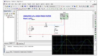
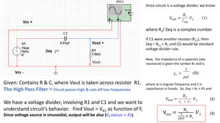
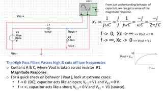
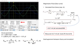
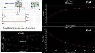
ANALYSIS of a HIGH PASS FILTER
Part 1 of 2
Given: Contains R & C, where Vout is taken across resistor R1.
The High Pass Filter ≡ Circuit passes high & cuts off low frequencies
We have a voltage divider, involving R1 and C1 and we want to
understand circuit’s behavior. Find Vout = VR1 as function of f;
Since voltage source is sinusoidal, output will be also (𝑉0 sin 𝜔𝑡 + 𝜃 ).
Since circuit is a voltage divider, we know:
𝑉out =
𝑅1
𝑍𝑒𝑞
𝑉1
where R1/ Zeq is a complex number.
If C1 were another resistor (RC1), then
Zeq = RC1 + R1 and (1) would be standard
voltage divider rule.
Now, the impedance of a capacitor (aka
reactance) is given the symbol Xc and is
𝜒𝑐 =
1
𝑗𝑤𝐶
where w is angular frequency and C is
capacitance in Farads. So, Zeq = Xc + R1 and
𝑉out =
𝑅1
𝑋𝑐 + 𝑅1
𝑉1
Vout =
R1
1
𝑗𝑤𝐶
+ 𝑅1
𝑉1
Zeq ┌>
(Ω)
(1)
(2)
(3)
The High Pass Filter: Passes high & cuts off low frequencies
o Contains R & C, where Vout is taken across resistor R1.
Magnitude Response:
o For a quick check on behavior |Vout|, look at extreme cases:
• f -> 0 (DC), capacitor acts like an open; VC 1 = V1 and VR1 = 0 V.
• f -> ∞, capacitor acts like a short; VC 1 = 0 V and VR1 = V1 (source).
𝑥𝑐 =
1
𝑗𝜔𝐶
=
𝑗
𝑗
⋅
1
𝑗𝑤𝐶
=
−𝑗
𝜔𝐶
=
−𝑗
2𝜋𝑓𝐶
f -> 0, Xc -> ∞ => Vout = 0 V
f -> ∞, Xc -> 0 => Vout = V1
Vout = VR1
f →
v1
From just understanding behavior of
capacitor, we can get a sense of the
magnitude response.
The High Pass Filter: Passes high & cuts off low frequencies
Phase Response
We can use phasor math to quickly analyze the phase behavior of Vout.
A phasor, 𝑧 = 𝑧 ∡𝜃, is another way to represent a complex number &
allows for quick calculation when multiplying and/or dividing.
𝑧𝑚 = 𝑧1𝑧2 = 𝑧1 ∡𝜃1 ∗ 𝑧2 ∡𝜃2 = 𝑧1 𝑧2 ∡ 𝜃1 + 𝜃2
𝑧𝐷 =
𝑧1
𝑧2
=
𝑧1 ∡𝜃1
𝑧2 ∡𝜃2
=
𝑧1
|𝑧2|
∡ 𝜃1 − 𝜃2
𝑅∡𝑜𝑜
𝑧𝑒𝑞 = |𝑧𝑒𝑞|∡ − 𝜃𝑒𝑞
Vout =
𝐑𝟏
𝟏
𝒋𝒘𝑪
+ 𝑹𝟏
𝑽𝟏
𝑧eq = 𝑅∡𝑂0 +
−𝑗
𝜔𝐶
= 𝑅 −
1
𝜔𝐶
𝑗 = 𝑧𝑒𝑞 ∡ − 𝜃𝑒𝑞
𝑉out =
𝑅1∡00
𝑧𝑒𝑞 ∡ − 𝜃𝑒𝑞
𝑉1∡00
𝑉out =
𝑅1
𝑧eq
∡0o
− −𝜃e𝑞
𝑜
𝑉1∡𝑂0
=
𝑅1
|𝑍𝑒𝑞|
∡𝜃e𝑞
𝑜
⋅ 𝑉1
V𝑜𝑢𝑡 ∡𝜃𝑒𝑞
This means that Vout leads V1!
𝑥𝑐 =
1
𝑗𝑤𝐶
=
−𝑗
𝑤𝐶
θeq
-θeq
(3)
ANALYSIS of a HIGH PASS FILTER
Part 2 of 2
Zeq ┌>
Let’s look at oscilloscope data for our circuit:
Channel A is connected to V1 our voltage source (green curve).
Our voltage source is listed at 1V peak. Channel A is scaled at
500 mV/Div; green curve covers 2 Div = 500 mV x 2 = 1 Vpk.
Channel B is connected to Vout (blue curve).
Vout leads V1 as predicted in last slide.
Note channel A & B do not have same voltage scale.
Circuit parameters:
V1 = 1,000 mVpk = 1 VpK,
f = 1,000 Hz, R1 = 1kΩ, and C1 = 0.01 μF
Circuit parameters:
V1 = 1,000 mVpk = 1 VpK,
f = 1,000 Hz, R1 = 1kΩ, and C1 = 0.01 μF
Vout =
R1
1
𝑗𝑤𝐶
+ 𝑅1
𝑉1 (3)
Magnitude of Vout (blue curve):
• Calculated from theory (eqn. 4):
• Measured: 62.7 mV pK (read off channel B)
Good agreement between theory and simulation!
𝑽𝐨𝐮𝐭 =
𝑹𝟏
𝑹𝟏 −
𝟏
𝒘𝑪
𝒋
⋅ 𝑉1 (4)
𝑉𝑜𝑢𝑡 =
𝑅1
𝑍𝑒𝑞
⋅ 𝑉1 =
𝑅1
𝑅1
2
+
1
𝑤𝐶
2
⋅ 𝑉1
1 × 10³
1 × 10³ 2 +
1
2𝜋 ⋅ 1,000 ⋅ 0.01 × 10
− 6
2
⋅ 1𝑉𝑃𝑘
= 62.7 mV pK calculated/ANS.
-
𝑤 =
2𝜋
𝑇
=
2𝜋
1
𝑓
= 2𝜋𝑓
NOTE:
Circuit parameters:
V1 = 1,000 mVpk = 1 VpK,
f = 1,000 Hz, R1 = 1kΩ, and C1 = 0.01 μF
Vout =
R1
1
𝑗𝑤𝐶
+ 𝑅1
𝑉1 (3)
Phase of Vout (blue curve):
• Calculated from theory: Using phasors, we can
analyze equation (4) quickly.
Numerator is a real number whose value is R1. Real
numbers have a 0⁰ angle.
Denominator was left in cartesian coordinate form. To
find the angle we’ll use arctan Y/X.
𝑽𝐨𝐮𝐭 =
𝑹𝟏
𝑹𝟏 −
𝟏
𝒘𝑪
𝒋
⋅ 𝑉1 (4)
∡𝜃𝑑𝑒𝑛 = tan−1
𝑦
𝑥
= tan−1
−1
𝑤𝐶1
𝑅1
= tan−1
−1
𝜔𝑅1𝐶1
∡𝜃den = tan−1
−1
2𝜋 ⋅ 1000 ⋅ 1000 ⋅ 0.01 × 10
− 6
= −86.4⁰
∡𝜃𝑣0ut
= ∡𝜃𝑛𝑢𝑚 − ∡𝜃den = 0 − −86.40
= 86.4⁰
• Measured: ∡𝜃𝑉𝑜𝑢𝑡 = 𝜔𝑡 = 2𝜋𝑓𝑡
= 2𝜋 ⋅ 1000 ⋅ 238.64 × 1.0−6 ⋅
1800
Π
= 85.9
0
Vout
Vout
Bode plotter
Circuit behavior across range of frequencies

High pass filter analysis complete

  • 1.
    ANALYSIS of aHIGH PASS FILTER Part 1 of 2
  • 2.
    Given: Contains R& C, where Vout is taken across resistor R1. The High Pass Filter ≡ Circuit passes high & cuts off low frequencies We have a voltage divider, involving R1 and C1 and we want to understand circuit’s behavior. Find Vout = VR1 as function of f; Since voltage source is sinusoidal, output will be also (𝑉0 sin 𝜔𝑡 + 𝜃 ). Since circuit is a voltage divider, we know: 𝑉out = 𝑅1 𝑍𝑒𝑞 𝑉1 where R1/ Zeq is a complex number. If C1 were another resistor (RC1), then Zeq = RC1 + R1 and (1) would be standard voltage divider rule. Now, the impedance of a capacitor (aka reactance) is given the symbol Xc and is 𝜒𝑐 = 1 𝑗𝑤𝐶 where w is angular frequency and C is capacitance in Farads. So, Zeq = Xc + R1 and 𝑉out = 𝑅1 𝑋𝑐 + 𝑅1 𝑉1 Vout = R1 1 𝑗𝑤𝐶 + 𝑅1 𝑉1 Zeq ┌> (Ω) (1) (2) (3)
  • 3.
    The High PassFilter: Passes high & cuts off low frequencies o Contains R & C, where Vout is taken across resistor R1. Magnitude Response: o For a quick check on behavior |Vout|, look at extreme cases: • f -> 0 (DC), capacitor acts like an open; VC 1 = V1 and VR1 = 0 V. • f -> ∞, capacitor acts like a short; VC 1 = 0 V and VR1 = V1 (source). 𝑥𝑐 = 1 𝑗𝜔𝐶 = 𝑗 𝑗 ⋅ 1 𝑗𝑤𝐶 = −𝑗 𝜔𝐶 = −𝑗 2𝜋𝑓𝐶 f -> 0, Xc -> ∞ => Vout = 0 V f -> ∞, Xc -> 0 => Vout = V1 Vout = VR1 f → v1 From just understanding behavior of capacitor, we can get a sense of the magnitude response.
  • 4.
    The High PassFilter: Passes high & cuts off low frequencies Phase Response We can use phasor math to quickly analyze the phase behavior of Vout. A phasor, 𝑧 = 𝑧 ∡𝜃, is another way to represent a complex number & allows for quick calculation when multiplying and/or dividing. 𝑧𝑚 = 𝑧1𝑧2 = 𝑧1 ∡𝜃1 ∗ 𝑧2 ∡𝜃2 = 𝑧1 𝑧2 ∡ 𝜃1 + 𝜃2 𝑧𝐷 = 𝑧1 𝑧2 = 𝑧1 ∡𝜃1 𝑧2 ∡𝜃2 = 𝑧1 |𝑧2| ∡ 𝜃1 − 𝜃2 𝑅∡𝑜𝑜 𝑧𝑒𝑞 = |𝑧𝑒𝑞|∡ − 𝜃𝑒𝑞 Vout = 𝐑𝟏 𝟏 𝒋𝒘𝑪 + 𝑹𝟏 𝑽𝟏 𝑧eq = 𝑅∡𝑂0 + −𝑗 𝜔𝐶 = 𝑅 − 1 𝜔𝐶 𝑗 = 𝑧𝑒𝑞 ∡ − 𝜃𝑒𝑞 𝑉out = 𝑅1∡00 𝑧𝑒𝑞 ∡ − 𝜃𝑒𝑞 𝑉1∡00 𝑉out = 𝑅1 𝑧eq ∡0o − −𝜃e𝑞 𝑜 𝑉1∡𝑂0 = 𝑅1 |𝑍𝑒𝑞| ∡𝜃e𝑞 𝑜 ⋅ 𝑉1 V𝑜𝑢𝑡 ∡𝜃𝑒𝑞 This means that Vout leads V1! 𝑥𝑐 = 1 𝑗𝑤𝐶 = −𝑗 𝑤𝐶 θeq -θeq (3)
  • 5.
    ANALYSIS of aHIGH PASS FILTER Part 2 of 2
  • 6.
    Zeq ┌> Let’s lookat oscilloscope data for our circuit: Channel A is connected to V1 our voltage source (green curve). Our voltage source is listed at 1V peak. Channel A is scaled at 500 mV/Div; green curve covers 2 Div = 500 mV x 2 = 1 Vpk. Channel B is connected to Vout (blue curve). Vout leads V1 as predicted in last slide. Note channel A & B do not have same voltage scale. Circuit parameters: V1 = 1,000 mVpk = 1 VpK, f = 1,000 Hz, R1 = 1kΩ, and C1 = 0.01 μF
  • 7.
    Circuit parameters: V1 =1,000 mVpk = 1 VpK, f = 1,000 Hz, R1 = 1kΩ, and C1 = 0.01 μF Vout = R1 1 𝑗𝑤𝐶 + 𝑅1 𝑉1 (3) Magnitude of Vout (blue curve): • Calculated from theory (eqn. 4): • Measured: 62.7 mV pK (read off channel B) Good agreement between theory and simulation! 𝑽𝐨𝐮𝐭 = 𝑹𝟏 𝑹𝟏 − 𝟏 𝒘𝑪 𝒋 ⋅ 𝑉1 (4) 𝑉𝑜𝑢𝑡 = 𝑅1 𝑍𝑒𝑞 ⋅ 𝑉1 = 𝑅1 𝑅1 2 + 1 𝑤𝐶 2 ⋅ 𝑉1 1 × 10³ 1 × 10³ 2 + 1 2𝜋 ⋅ 1,000 ⋅ 0.01 × 10 − 6 2 ⋅ 1𝑉𝑃𝑘 = 62.7 mV pK calculated/ANS. - 𝑤 = 2𝜋 𝑇 = 2𝜋 1 𝑓 = 2𝜋𝑓 NOTE:
  • 8.
    Circuit parameters: V1 =1,000 mVpk = 1 VpK, f = 1,000 Hz, R1 = 1kΩ, and C1 = 0.01 μF Vout = R1 1 𝑗𝑤𝐶 + 𝑅1 𝑉1 (3) Phase of Vout (blue curve): • Calculated from theory: Using phasors, we can analyze equation (4) quickly. Numerator is a real number whose value is R1. Real numbers have a 0⁰ angle. Denominator was left in cartesian coordinate form. To find the angle we’ll use arctan Y/X. 𝑽𝐨𝐮𝐭 = 𝑹𝟏 𝑹𝟏 − 𝟏 𝒘𝑪 𝒋 ⋅ 𝑉1 (4) ∡𝜃𝑑𝑒𝑛 = tan−1 𝑦 𝑥 = tan−1 −1 𝑤𝐶1 𝑅1 = tan−1 −1 𝜔𝑅1𝐶1 ∡𝜃den = tan−1 −1 2𝜋 ⋅ 1000 ⋅ 1000 ⋅ 0.01 × 10 − 6 = −86.4⁰ ∡𝜃𝑣0ut = ∡𝜃𝑛𝑢𝑚 − ∡𝜃den = 0 − −86.40 = 86.4⁰ • Measured: ∡𝜃𝑉𝑜𝑢𝑡 = 𝜔𝑡 = 2𝜋𝑓𝑡 = 2𝜋 ⋅ 1000 ⋅ 238.64 × 1.0−6 ⋅ 1800 Π = 85.9 0
  • 9.
    Vout Vout Bode plotter Circuit behavioracross range of frequencies