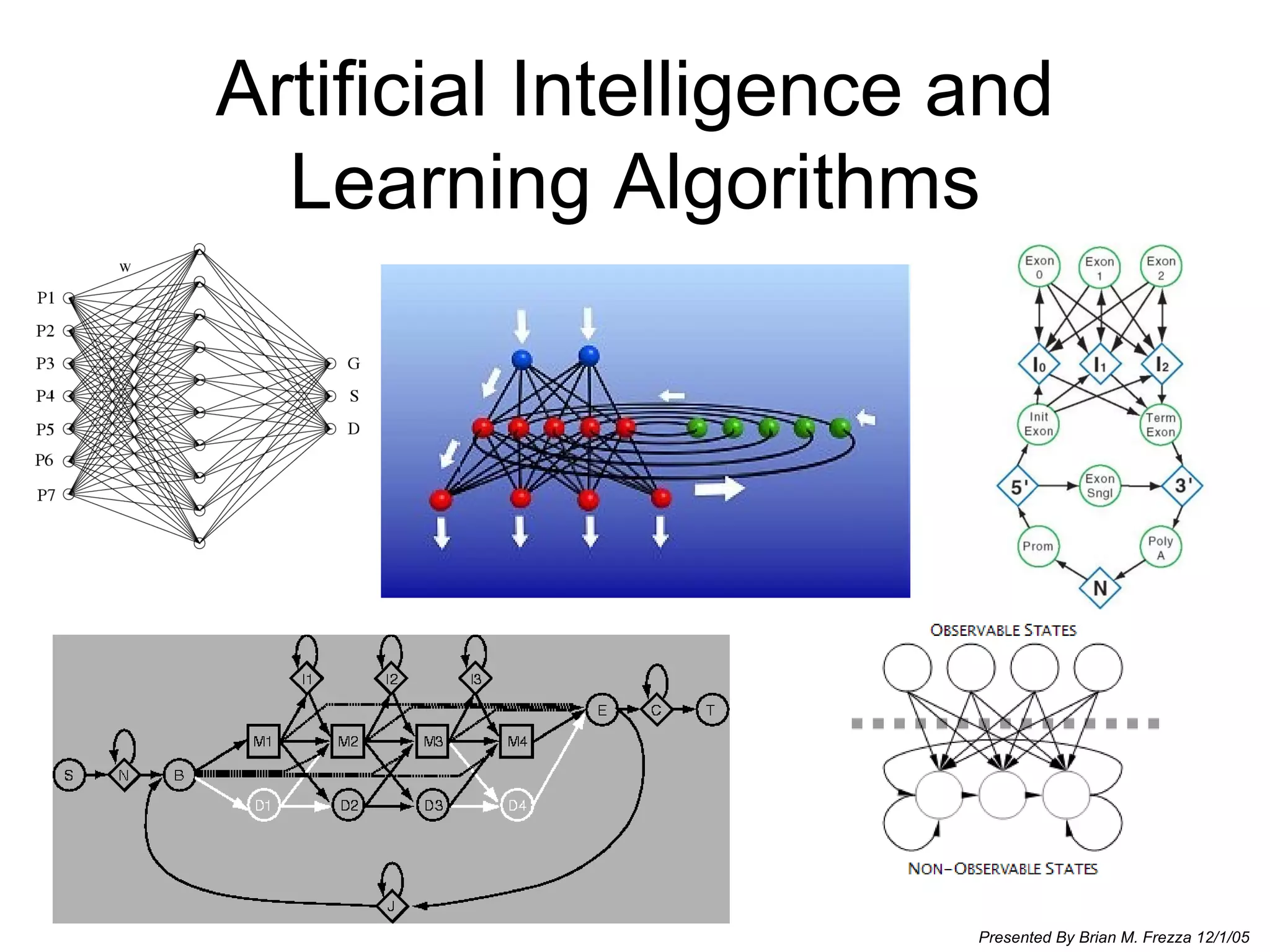
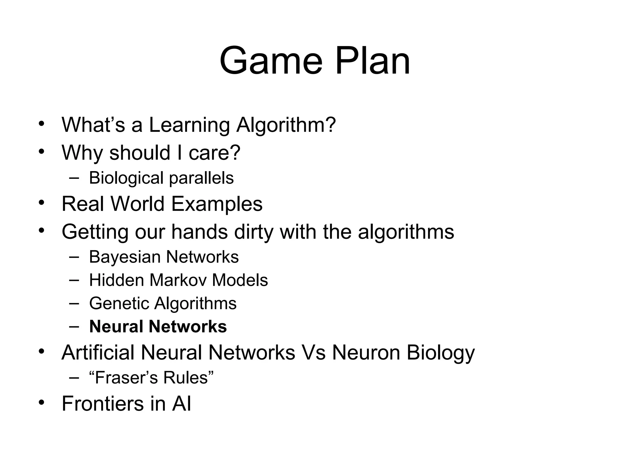
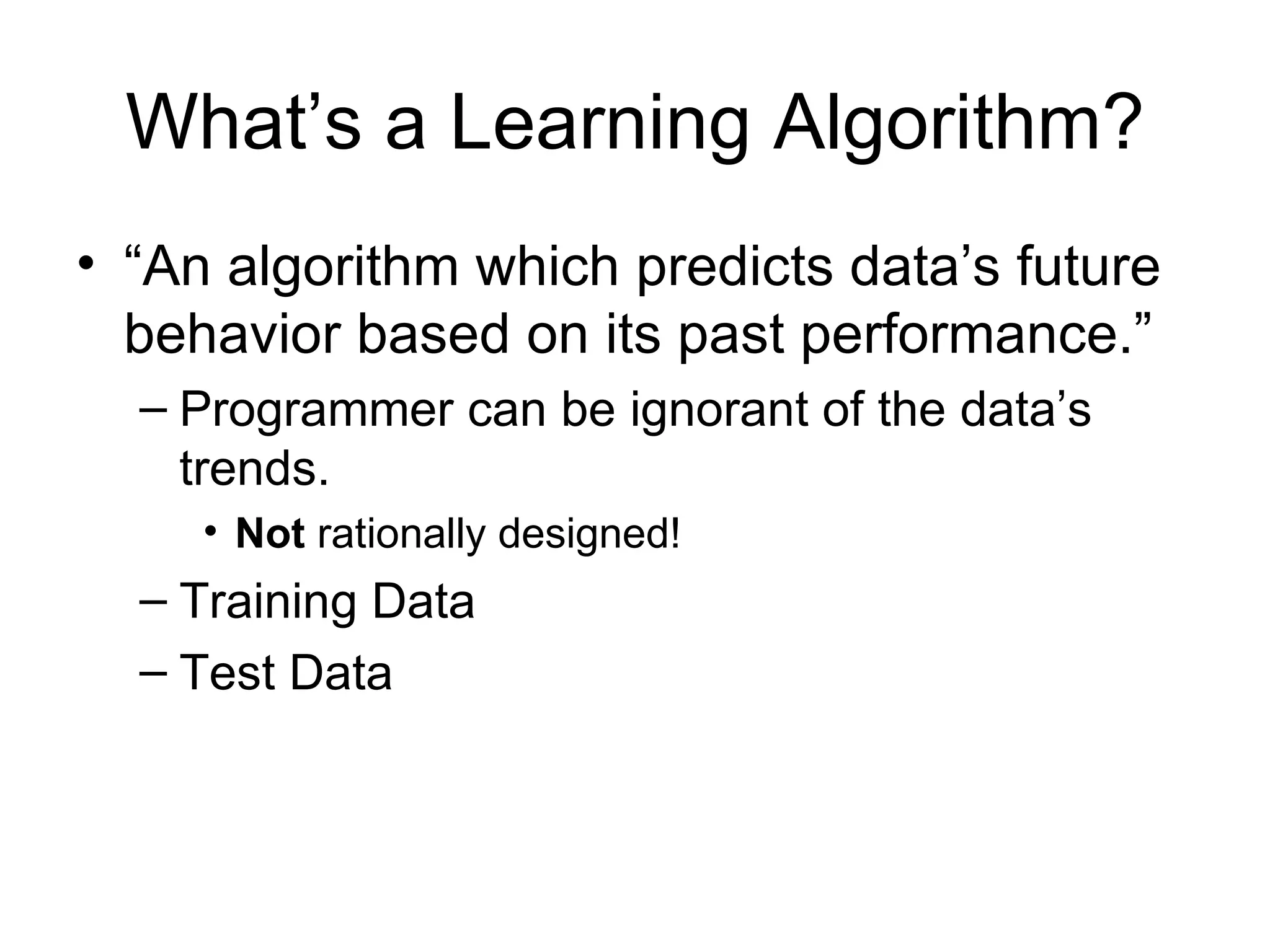
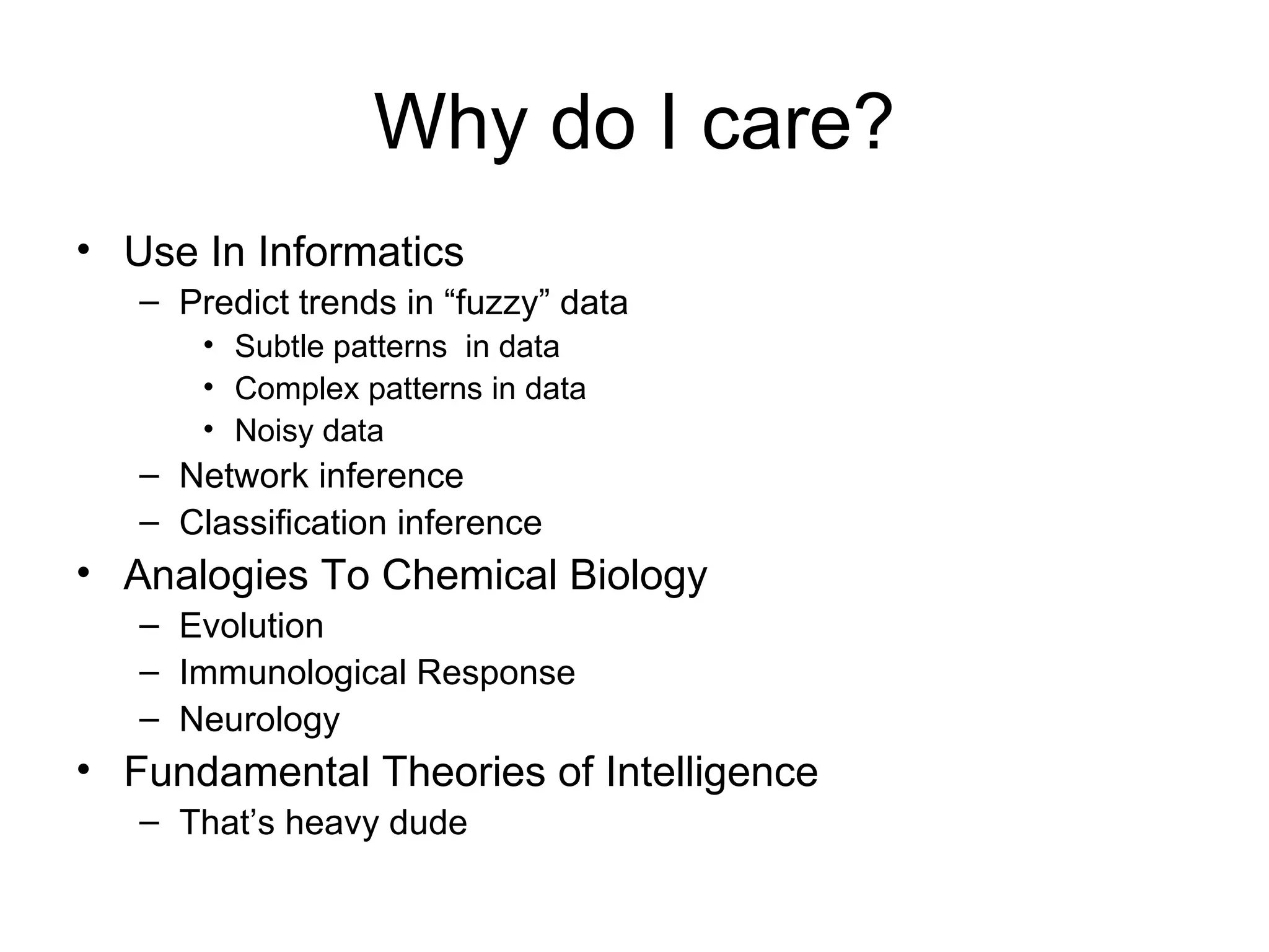
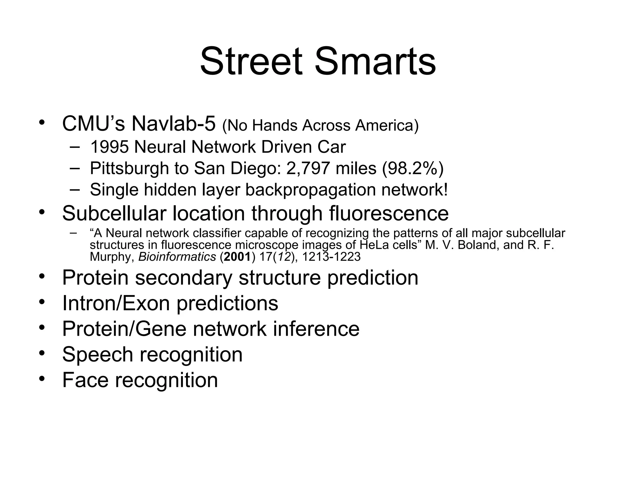
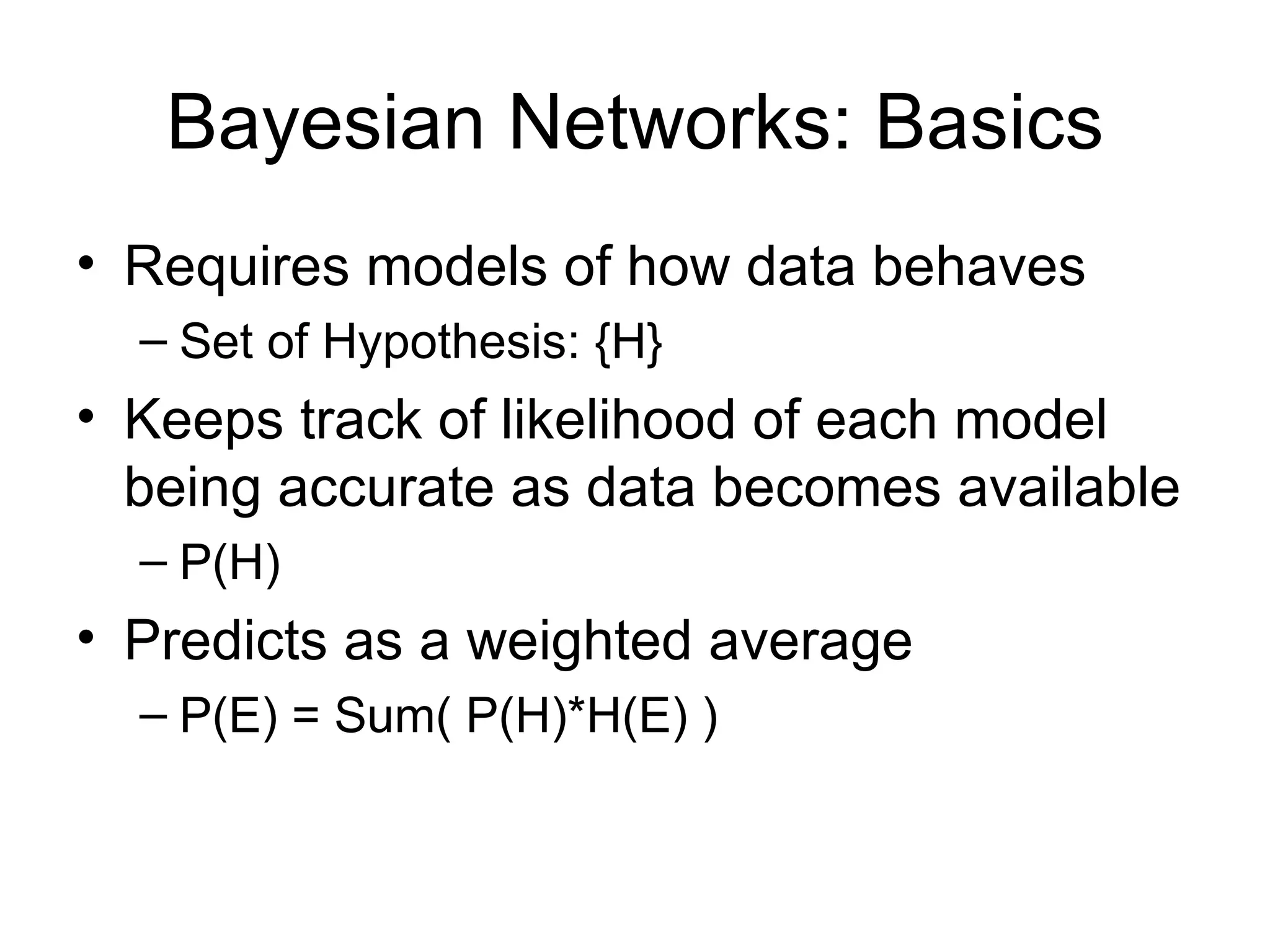
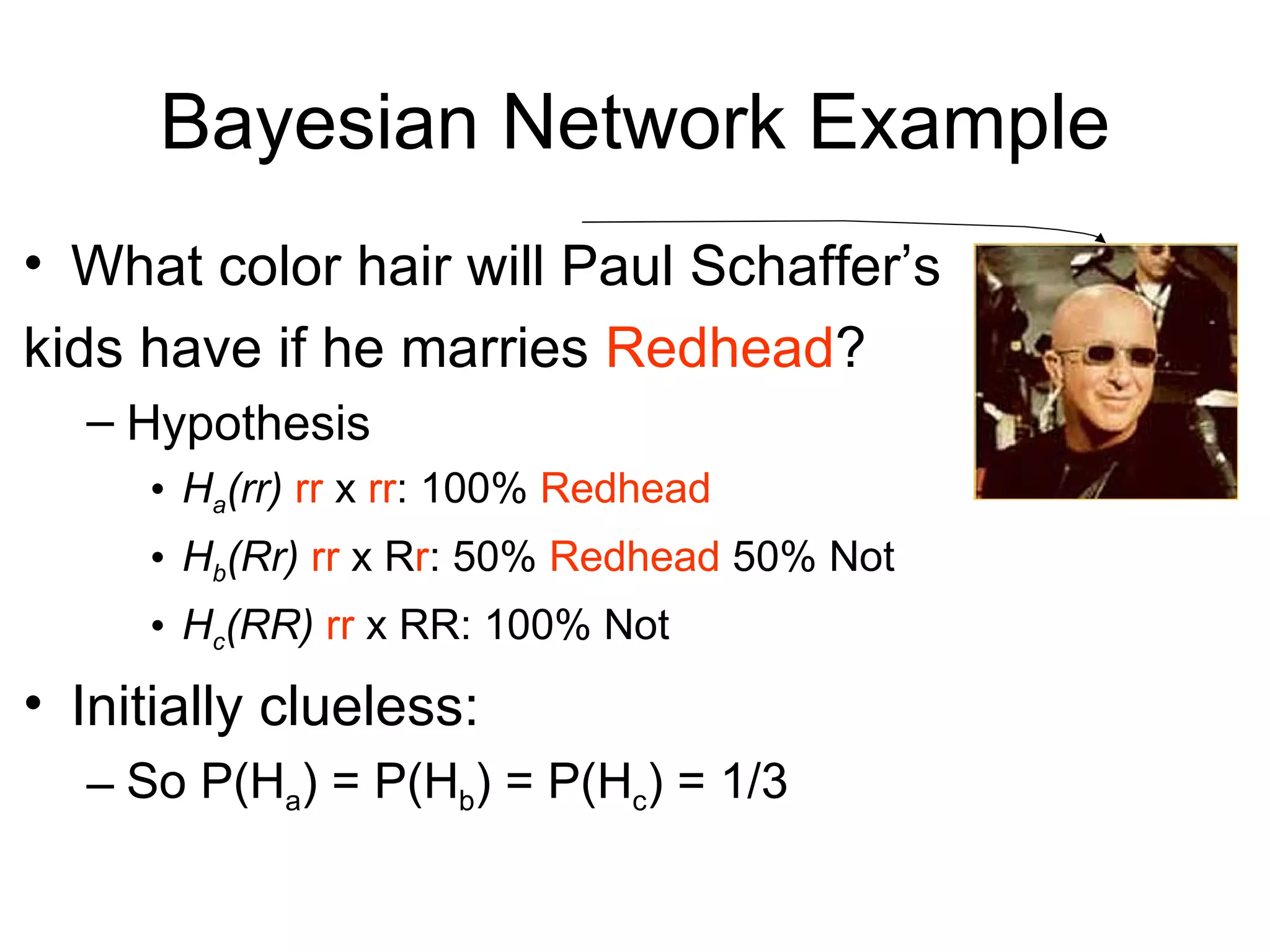
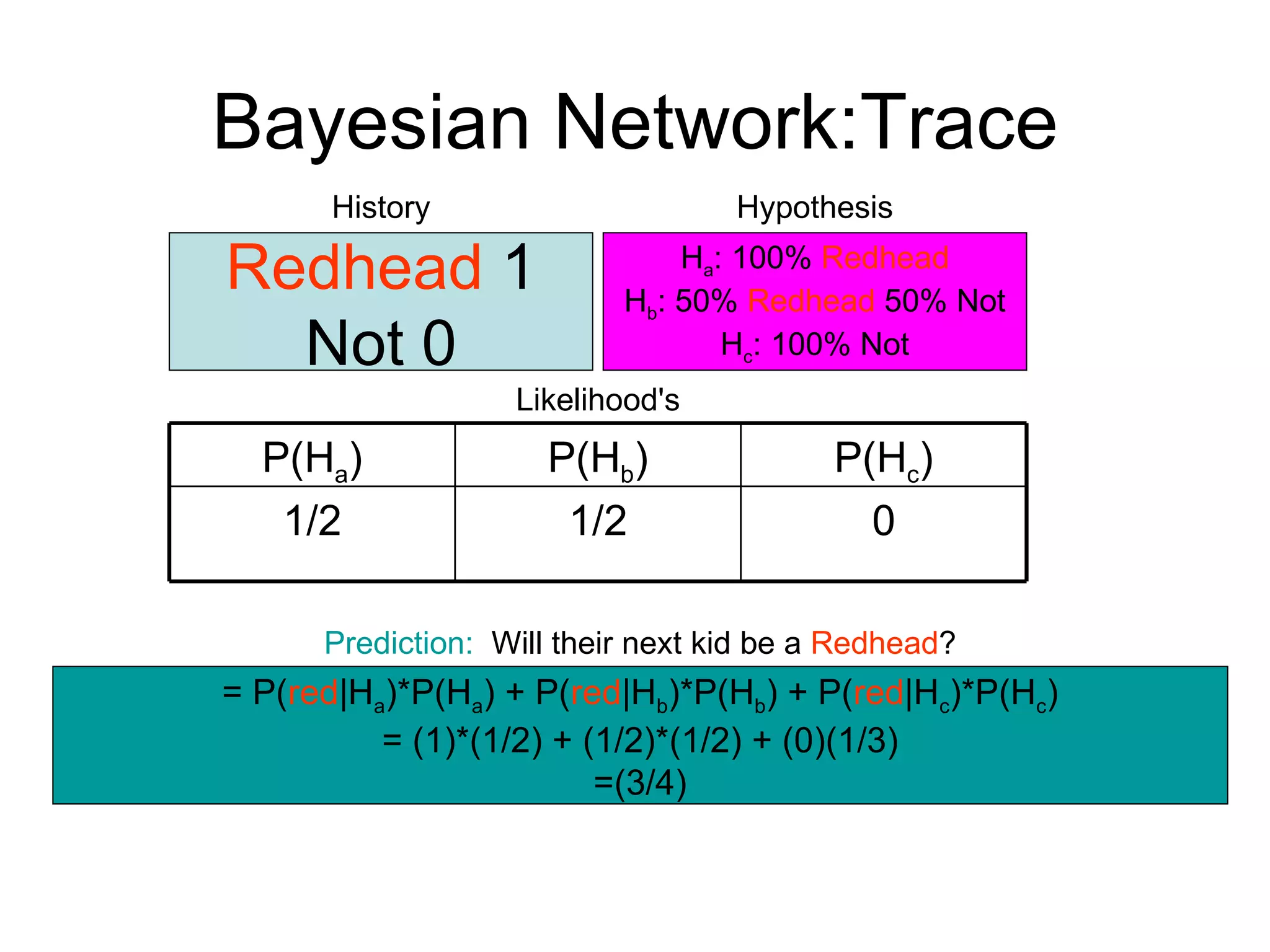
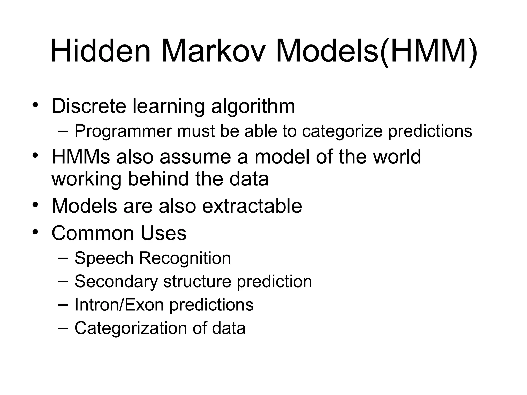
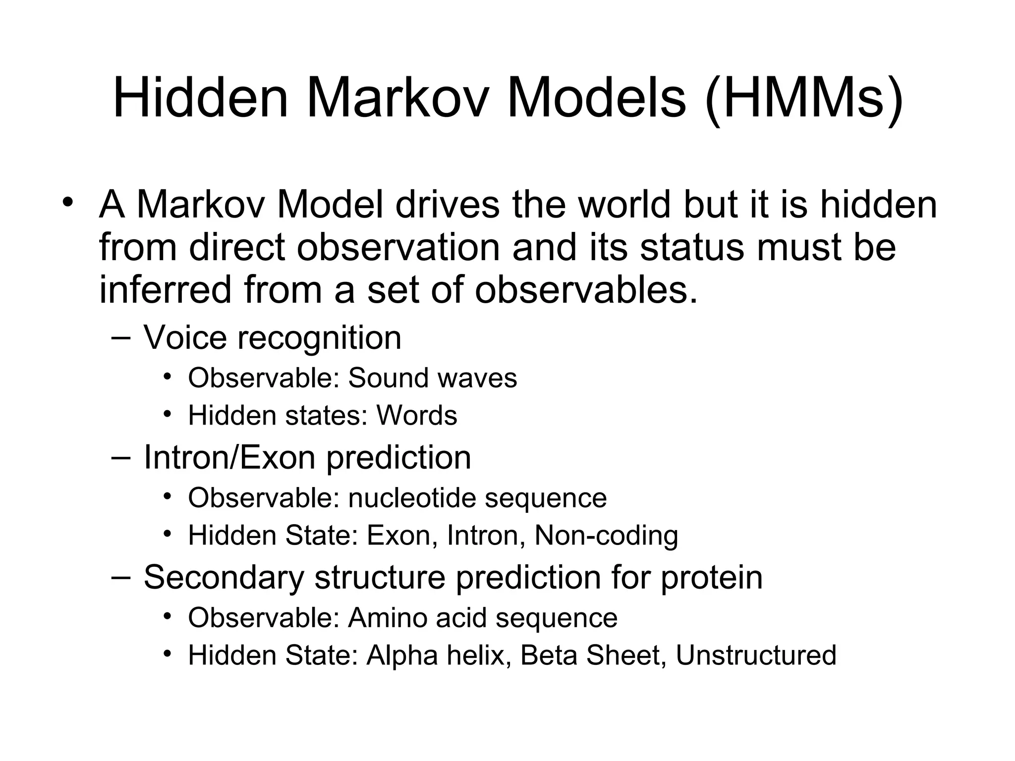
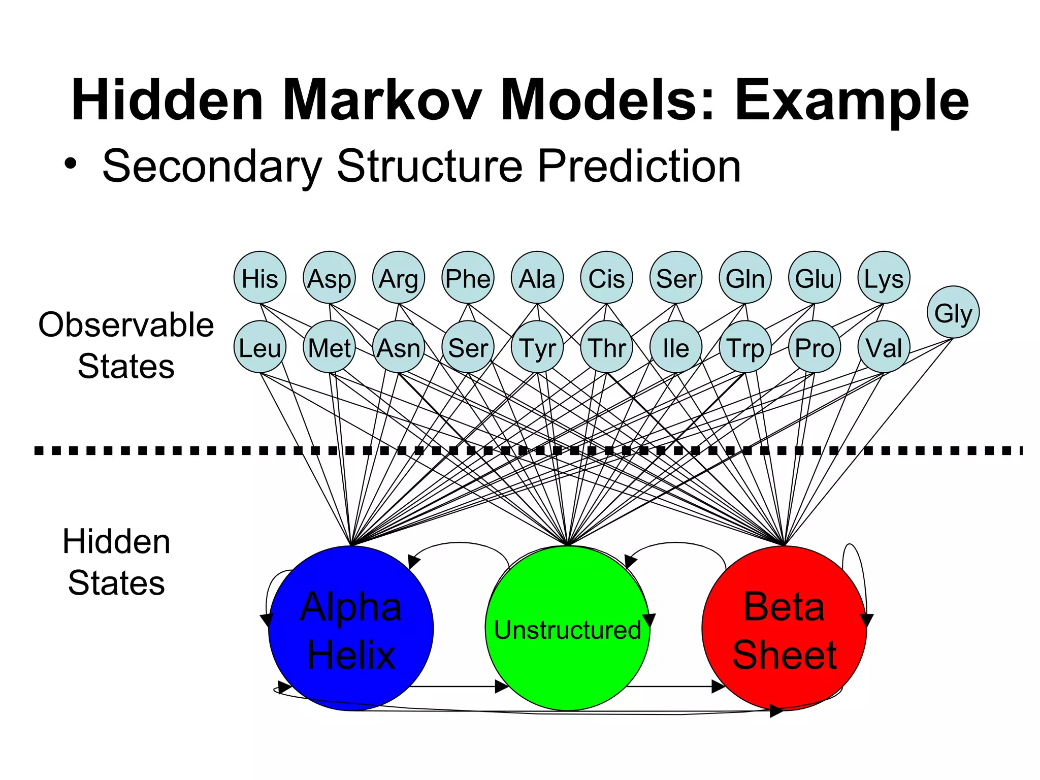
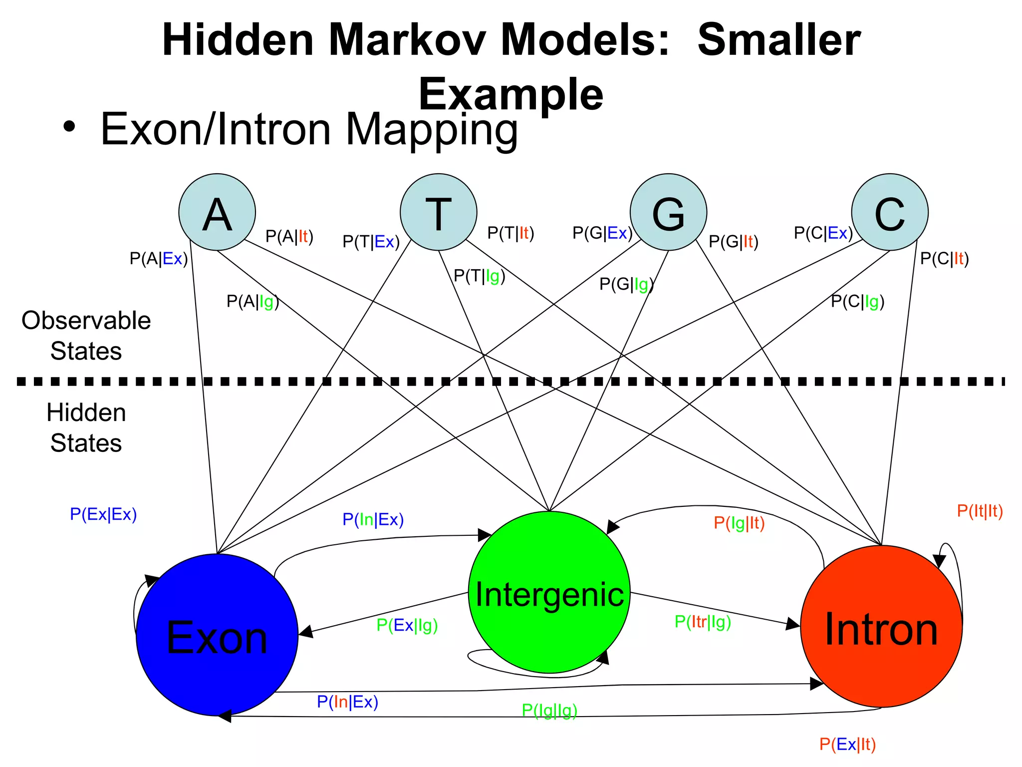
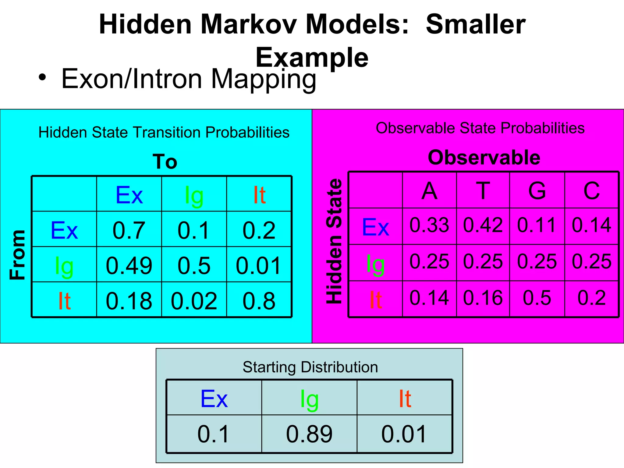
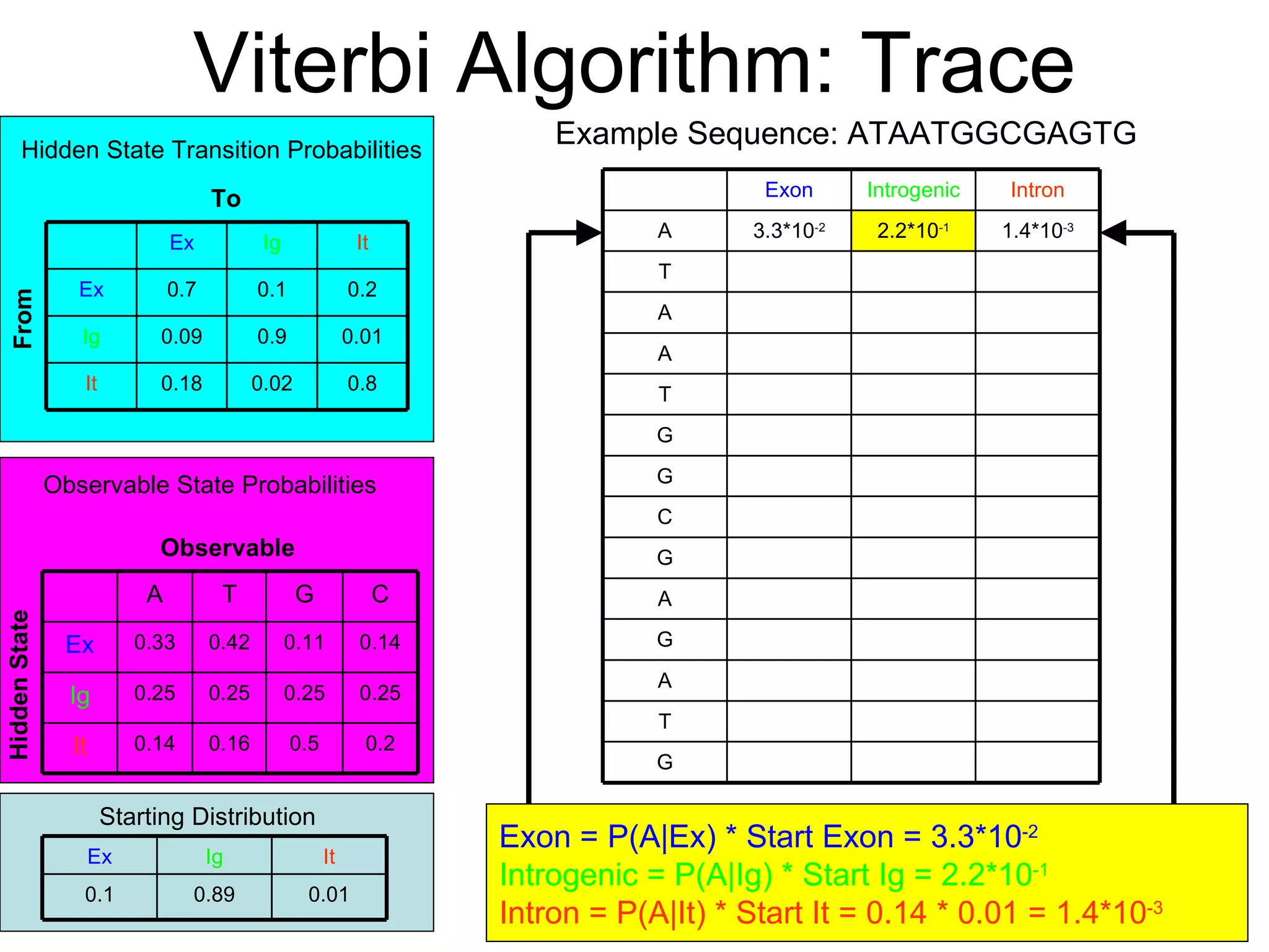
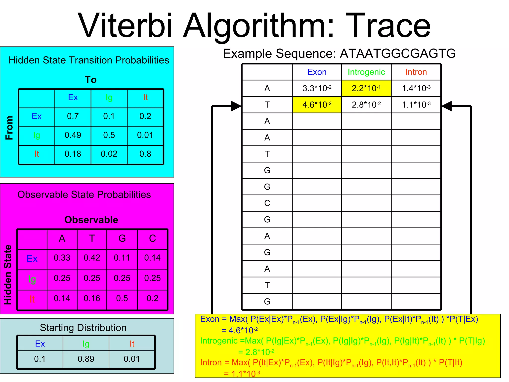
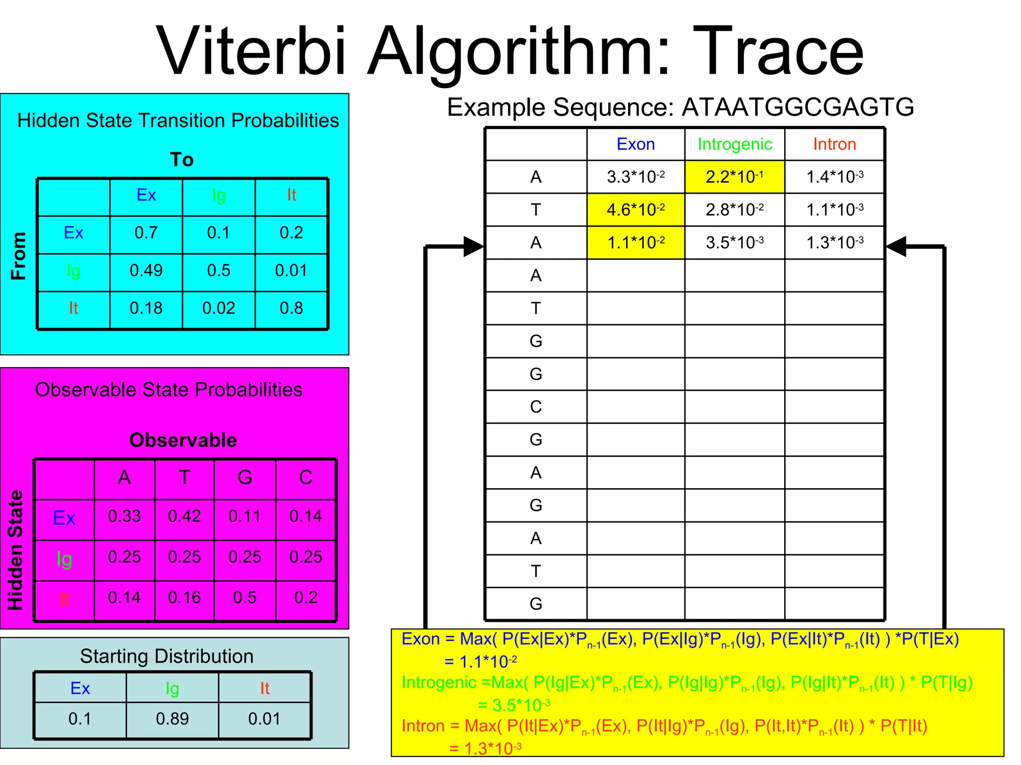
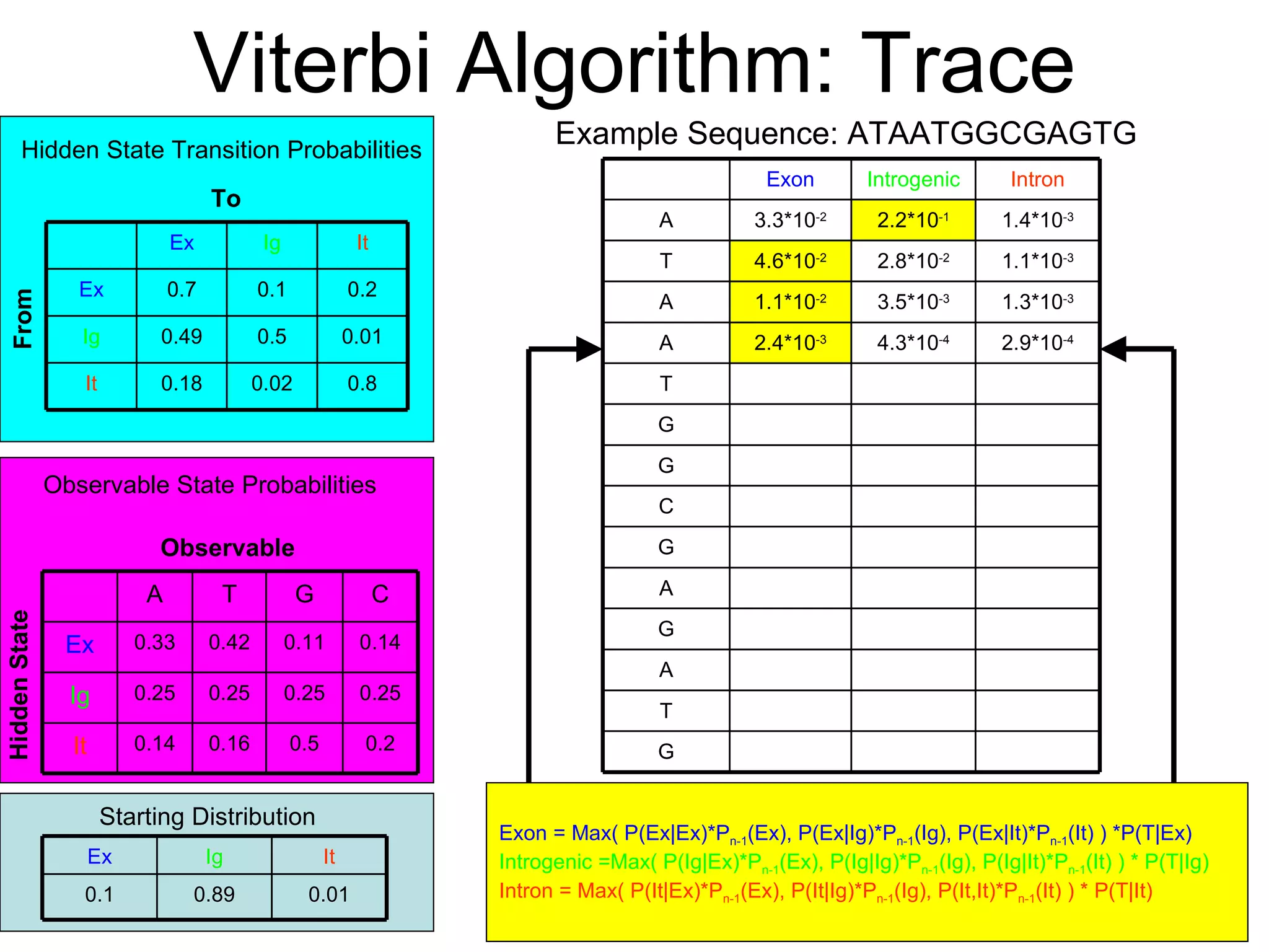
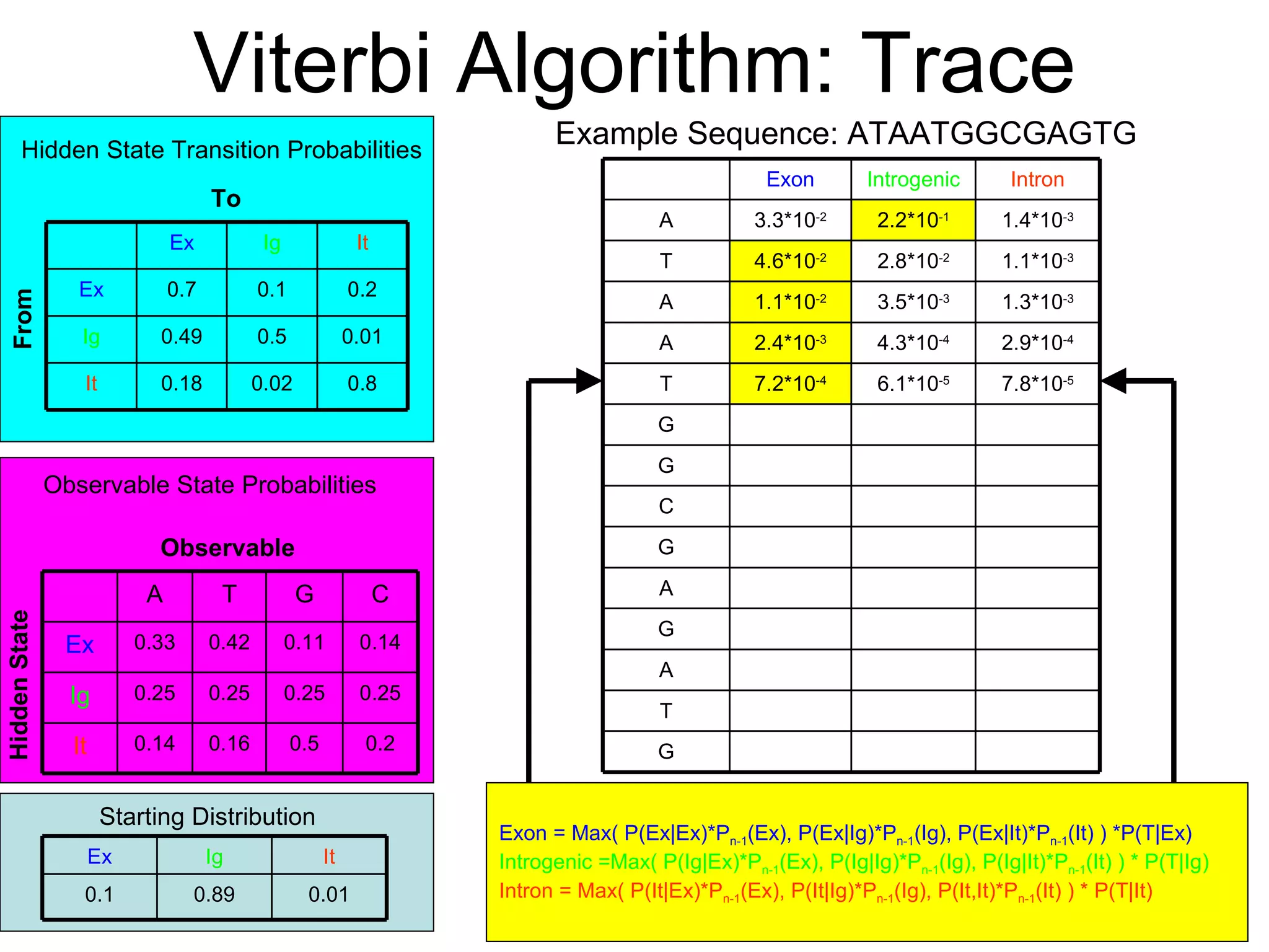
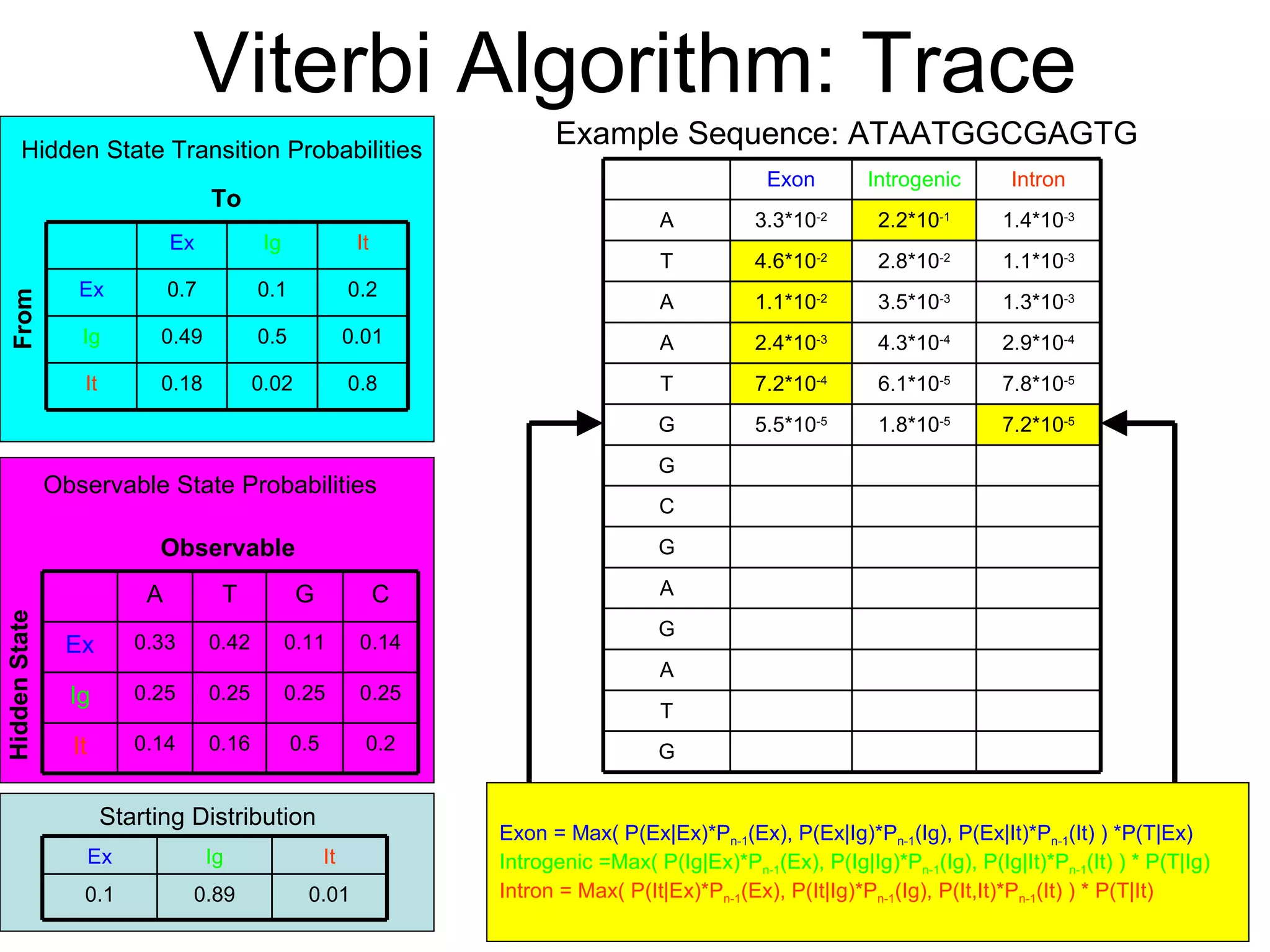
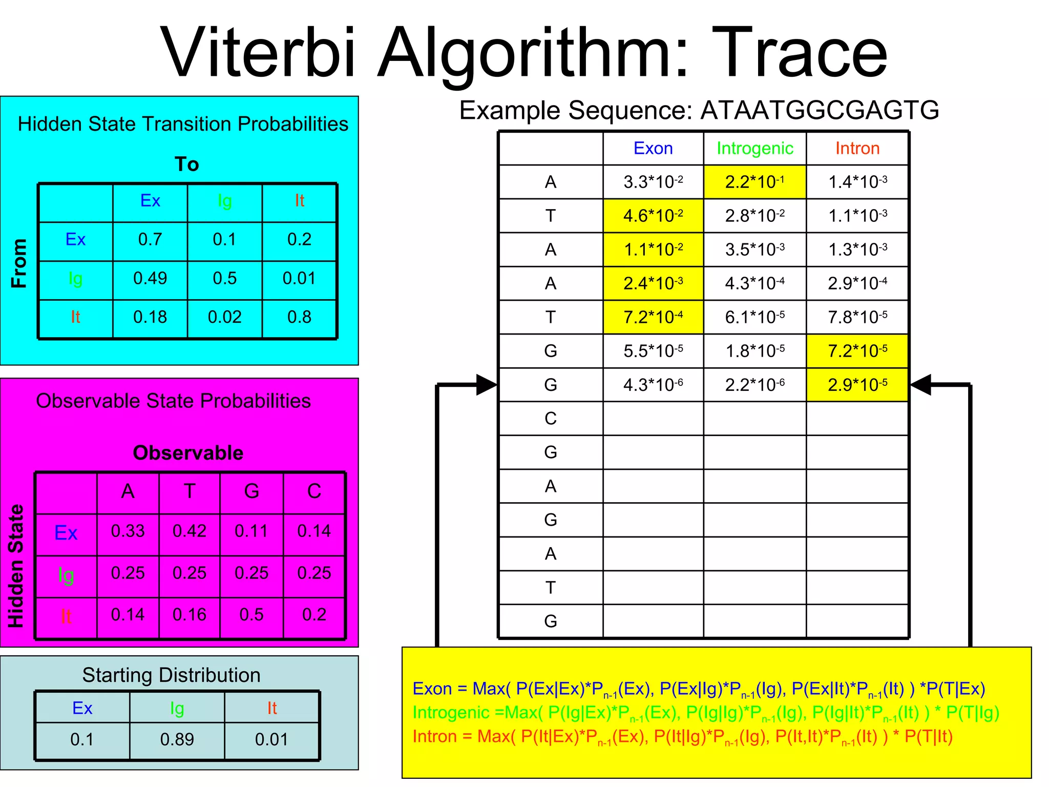
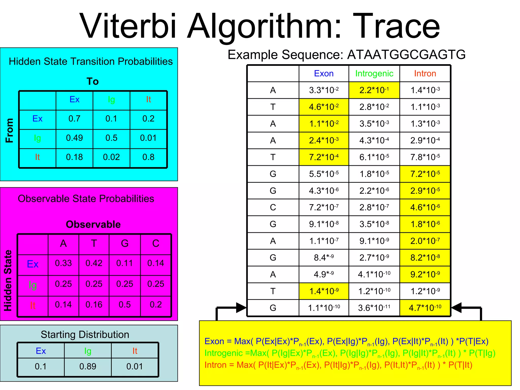
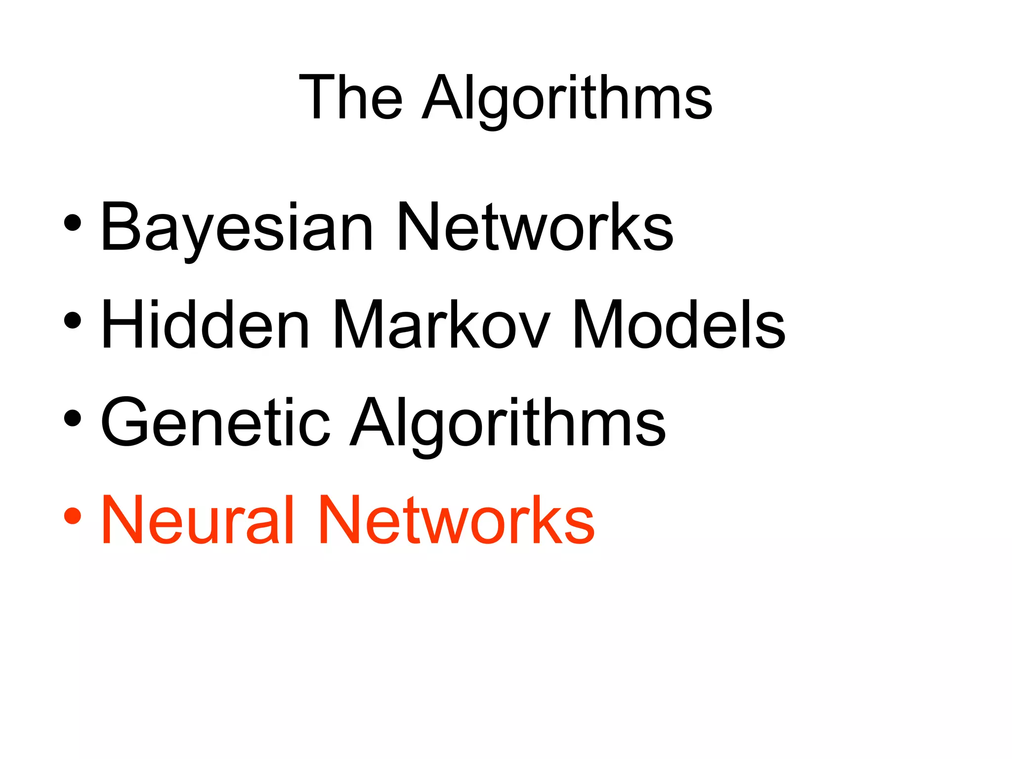
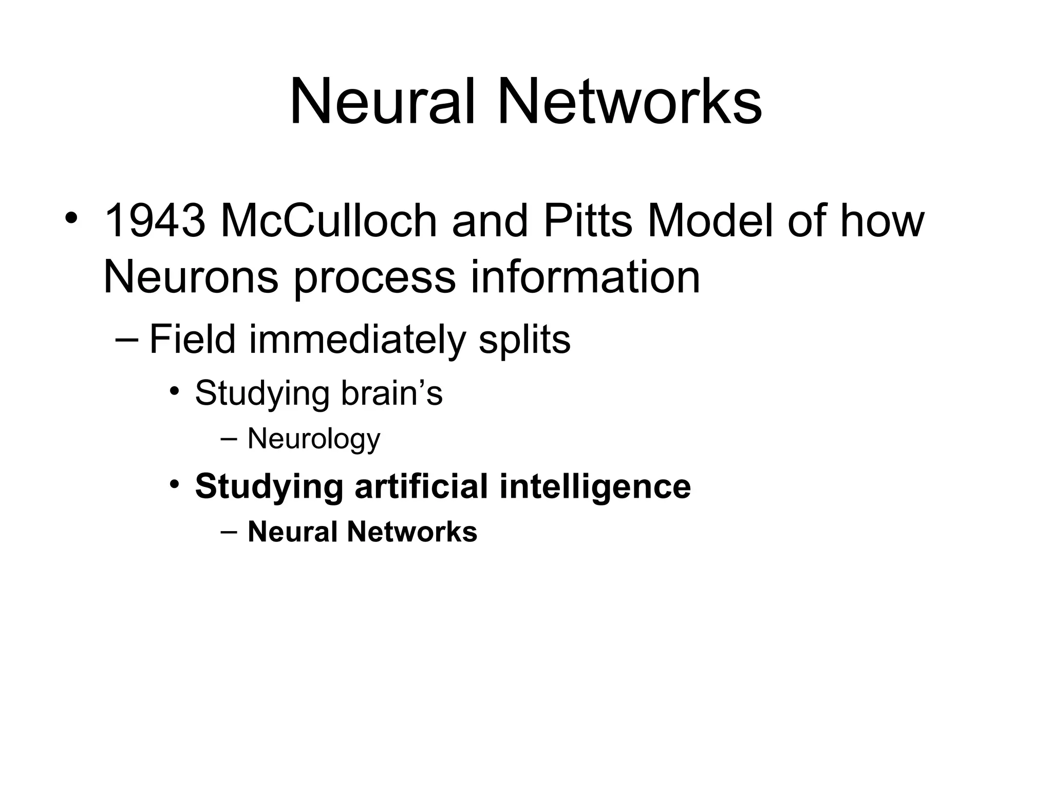
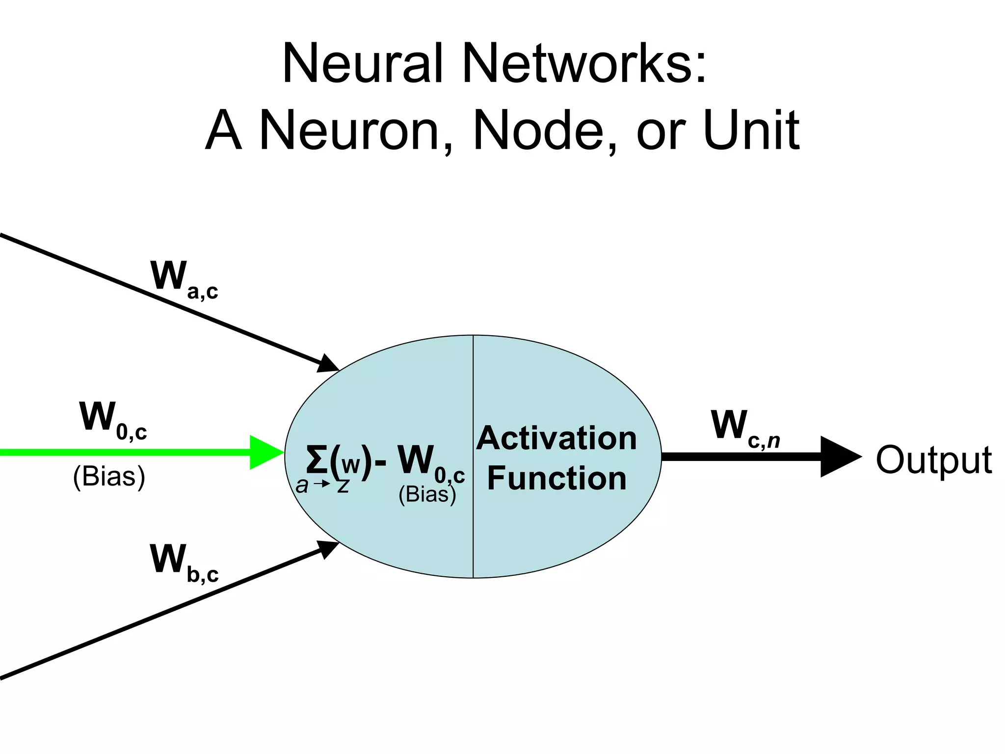
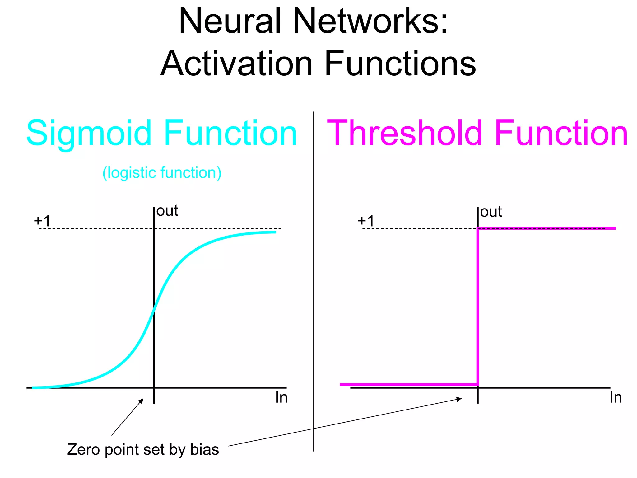
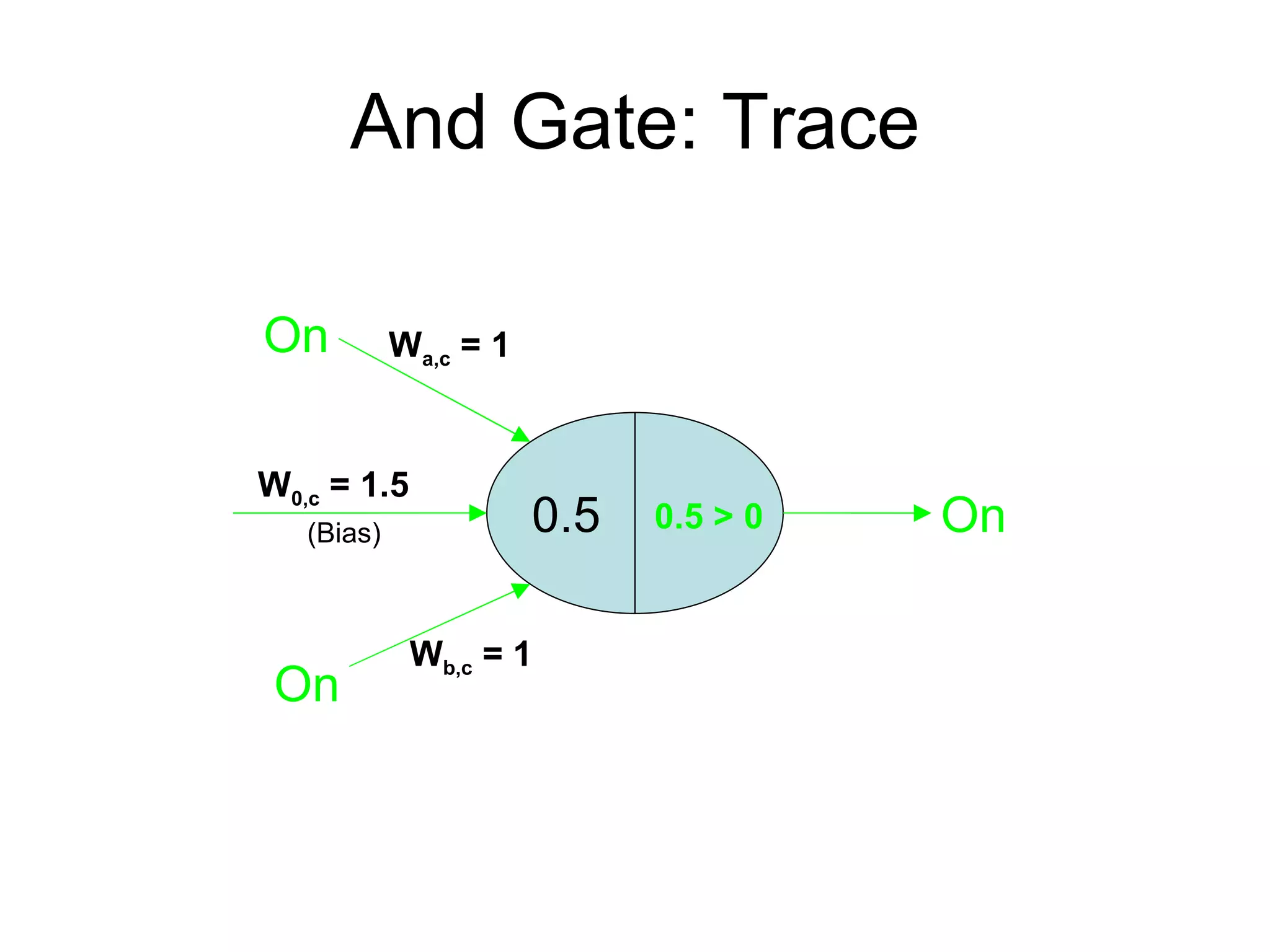
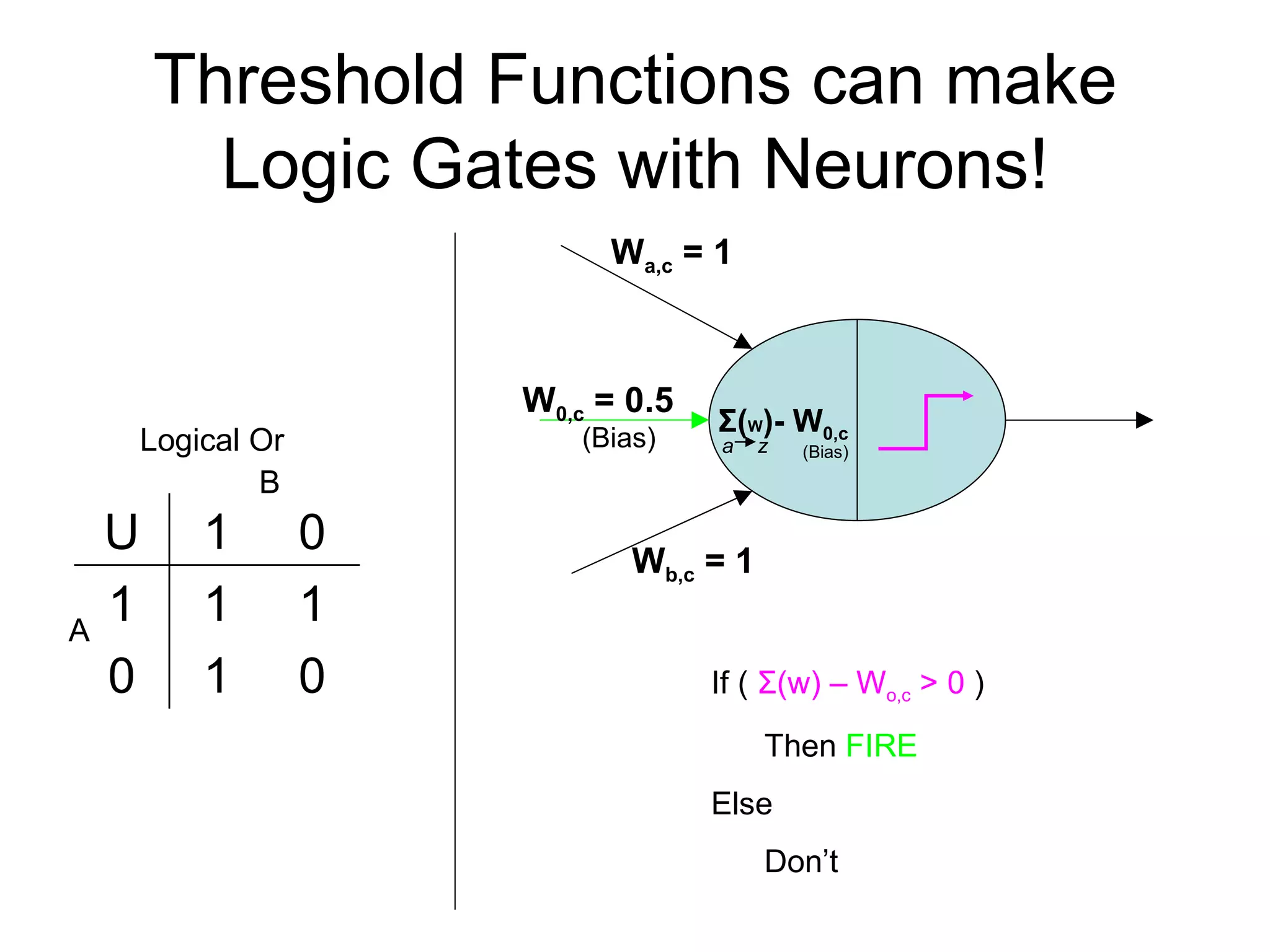
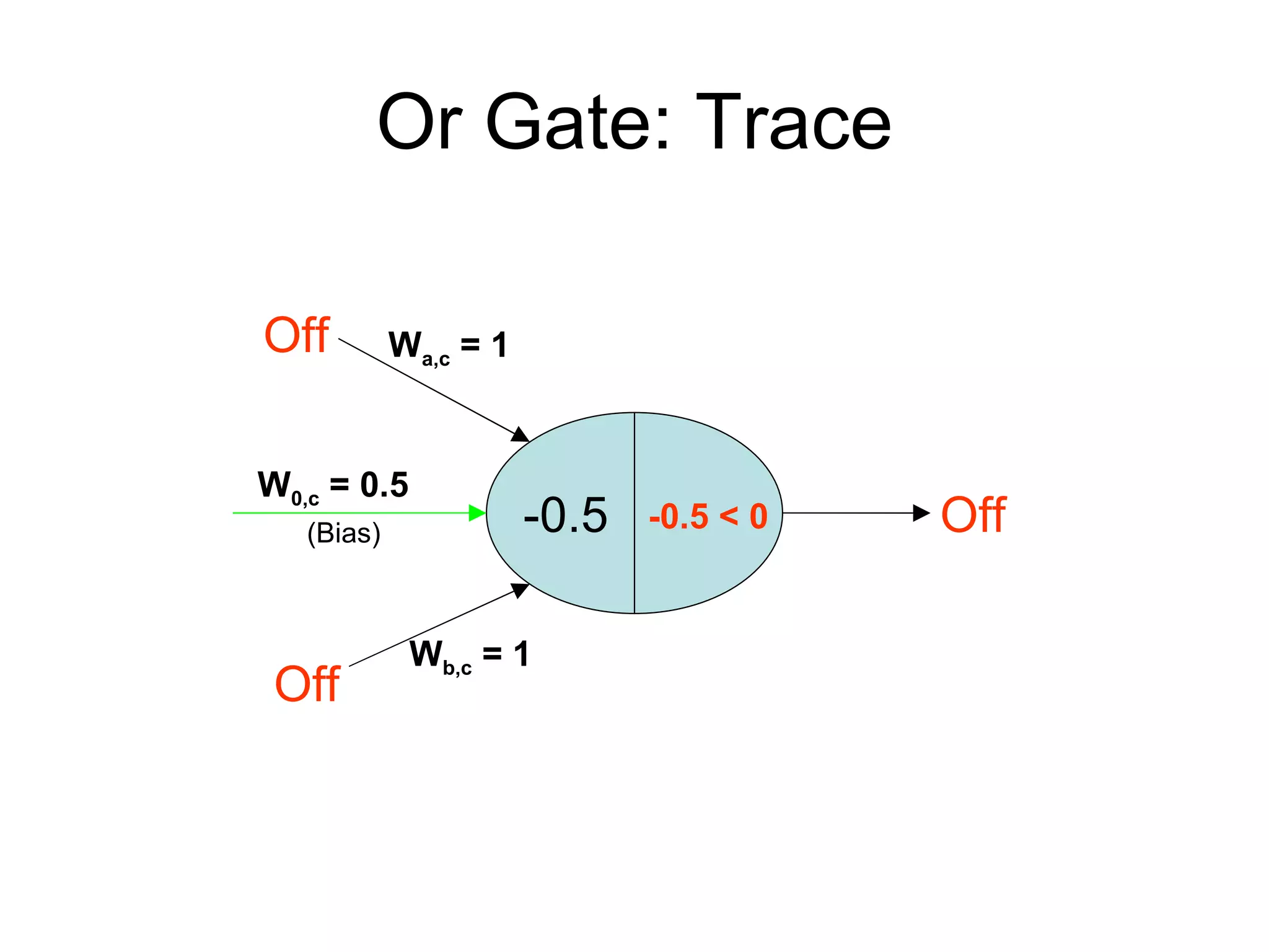
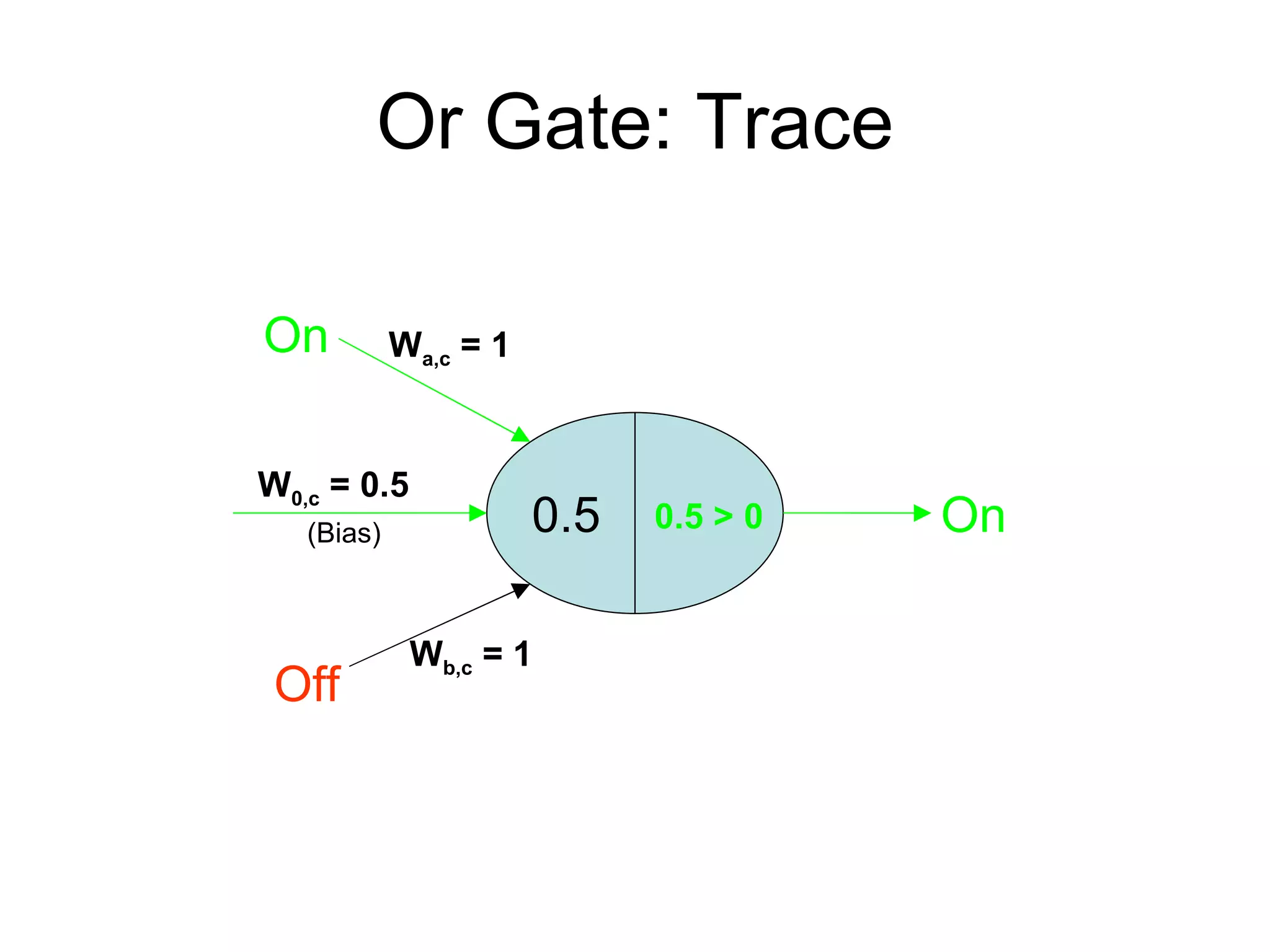
Brian M. Frezza's document explores learning algorithms in artificial intelligence, defining them as algorithms that predict data behavior based on past performance. It discusses various models such as Bayesian networks, hidden Markov models, genetic algorithms, and neural networks, alongside real-world applications like speech recognition and biological predictions. Additionally, it highlights the importance of training and testing data, and how these algorithms learn from data structures and patterns.

1. Artificial Intelligence and Learning Algorithms Presented By Brian M. Frezza 12/1/05

2. Game Plan What’s a Learning Algorithm? Why should I care? Biological parallels Real World Examples Getting our hands dirty with the algorithms Bayesian Networks Hidden Markov Models Genetic Algorithms Neural Networks Artificial Neural Networks Vs Neuron Biology “ Fraser’s Rules” Frontiers in AI

3. Hard Math

4. What’s a Learning Algorithm? “An algorithm which predicts data’s future behavior based on its past performance.” Programmer can be ignorant of the data’s trends. Not rationally designed! Training Data Test Data

5. Why do I care? Use In Informatics Predict trends in “fuzzy” data Subtle patterns in data Complex patterns in data Noisy data Network inference Classification inference Analogies To Chemical Biology Evolution Immunological Response Neurology Fundamental Theories of Intelligence That’s heavy dude

6. Street Smarts CMU’s Navlab-5 (No Hands Across America) 1995 Neural Network Driven Car Pittsburgh to San Diego: 2,797 miles (98.2%) Single hidden layer backpropagation network! Subcellular location through fluorescence “ A Neural network classifier capable of recognizing the patterns of all major subcellular structures in fluorescence microscope images of HeLa cells” M. V. Boland, and R. F. Murphy, Bioinformatics ( 2001 ) 17( 12 ), 1213-1223 Protein secondary structure prediction Intron/Exon predictions Protein/Gene network inference Speech recognition Face recognition

7. The Algorithms Bayesian Networks Hidden Markov Models Genetic Algorithms Neural Networks

8. Bayesian Networks: Basics Requires models of how data behaves Set of Hypothesis: {H} Keeps track of likelihood of each model being accurate as data becomes available P(H) Predicts as a weighted average P(E) = Sum( P(H)*H(E) )

9. Bayesian Network Example What color hair will Paul Schaffer’s kids have if he marries Redhead ? Hypothesis H a (rr) rr x rr : 100% Redhead H b (Rr) rr x R r : 50% Redhead 50% Not H c (RR) rr x RR: 100% Not Initially clueless: So P(H a ) = P(H b ) = P(H c ) = 1/3

10. Bayesian Network: Trace H a : 100% Redhead H b : 50% Redhead 50% Not H c : 100% Not Redhead 0 Not 0 Hypothesis History Likelihood's = P( red |H a )*P(H a ) + P( red |H b )*P(H b ) + P( red |H c )*P(H c ) = (1)*(1/3) + (1/2)*(1/3) + (0)(1/3) =(1/2) Prediction: Will their next kid be a Redhead ? 1/3 1/3 1/3 P(H c ) P(H b ) P(H a )

11. Bayesian Network:Trace H a : 100% Redhead H b : 50% Redhead 50% Not H c : 100% Not Redhead 1 Not 0 Hypothesis History Likelihood's = P( red |H a )*P(H a ) + P( red |H b )*P(H b ) + P( red |H c )*P(H c ) = (1)*(1/2) + (1/2)*(1/2) + (0)(1/3) =(3/4) Prediction: Will their next kid be a Redhead ? 0 1/2 1/2 P(H c ) P(H b ) P(H a )

12. Bayesian Network: Trace H a : 100% Redhead H b : 50% Redhead 50% Not H c : 100% Not Redhead 2 Not 0 Hypothesis History Likelihood's = P( red |H a )*P(H a ) + P( red |H b )*P(H b ) + P( red |H c )*P(H c ) = (1)*(3/4) + (1/2)*(1/4) + (0)(1/3) =(7/8) Prediction: Will their next kid be a Redhead ? 0 1/4 3/4 P(H c ) P(H b ) P(H a )

13. Bayesian Network: Trace H a : 100% Redhead H b : 50% Redhead 50% Not H c : 100% Not Redhead 3 Not 0 Hypothesis History Likelihood's = P( red |H a )*P(H a ) + P( red |H b )*P(H b ) + P( red |H c )*P(H c ) = (1)*(7/8) + (1/2)*(1/8) + (0)(1/3) =(15/16) Prediction: Will their next kid be a Redhead ? 0 1/8 7/8 P(H c ) P(H b ) P(H a )

14. Bayesian Networks Notes Never reject hypothesis unless directly disproved Learns based on rational models of behavior Models can be extracted! Programmer needs to form hypothesis beforehand.

15. The Algorithms Bayesian Networks Hidden Markov Models Genetic Algorithms Neural Networks

16. Hidden Markov Models(HMM) Discrete learning algorithm Programmer must be able to categorize predictions HMMs also assume a model of the world working behind the data Models are also extractable Common Uses Speech Recognition Secondary structure prediction Intron/Exon predictions Categorization of data

17. Hidden Markov Models: Take a Step Back 1 st order Markov Models: Q{States} Pr{Transition} Sum of all P(T) out of state = 1 Q 1 Q 4 Q 2 Q 3 P 1 P 2 1-P 1 -P 2 P 3 1-P 3 1 1-P 4 P 4

18. 1 st order Markov Model Setup Pick Initial state: Q 1 Pick Transition Probabilities: For each time step Pick a random number 0.0-1.0 Q 1 Q 4 Q 2 Q 3 P 1 P 2 1-P 1 -P 2 P 3 1-P 3 1 1-P 4 P 4 P 1 P 2 P 3 P 4 0.6 0.2 0.9 0.4

19. 1 st order Markov Model Trace Current State: Q 1 Time Step = 1 Transition probabilities: Random Number: 0.22341 So Next State: 0.22341 < P 1 Take P 1 Q 2 Q 1 Q 4 Q 2 Q 3 P 1 P 2 1-P 1 -P 2 P 3 1-P 3 1 1-P 4 P 4 P 1 P 2 P 3 P 4 0.6 0.2 0.9 0.4

20. 1 st order Markov Model Trace Current State: Q 2 Time Step = 2 Transition probabilities: Random Number: 0.64357 So Next State: No Choice, P = 1 Q 3 Q 1 Q 4 Q 2 Q 3 P 1 P 2 1-P 1 -P 2 P 3 1-P 3 1 1-P 4 P 4 P 1 P 2 P 3 P 4 0.6 0.2 0.9 0.4

21. 1 st order Markov Model Trace Current State: Q 3 Time Step = 3 Transition probabilities: Random Number: 0.97412 So Next State: 0.97412 > 0.9 Take 1-P 3 Q 4 Q 1 Q 4 Q 2 Q 3 P 1 P 2 1-P 1 -P 2 P 3 1-P 3 1 1-P 4 P 4 P 1 P 2 P 3 P 4 0.6 0.2 0.9 0.4

22. 1 st order Markov Model Trace Current State: Q 4 Time Step = 4 Transition probabilities: I’m going to stop here. Markov Chain: Q 1 , Q 2 , Q 3 , Q 4 Q 1 Q 4 Q 2 Q 3 P 1 P 2 1-P 1 -P 2 P 3 1-P 3 1 1-P 4 P 4 P 1 P 2 P 3 P 4 0.6 0.2 0.9 0.4

23. What else can Markov do? Higher Order Models K th order Metropolis-Hastings Determining thermodynamic equilibrium Continuous Markov Models Time step varies according to continuous distribution Hidden Markov Models Discrete model learning

24. Hidden Markov Models (HMMs) A Markov Model drives the world but it is hidden from direct observation and its status must be inferred from a set of observables. Voice recognition Observable: Sound waves Hidden states: Words Intron/Exon prediction Observable: nucleotide sequence Hidden State: Exon, Intron, Non-coding Secondary structure prediction for protein Observable: Amino acid sequence Hidden State: Alpha helix, Beta Sheet, Unstructured

25. Hidden Markov Models: Example Secondary Structure Prediction Observable States Hidden States Unstructured Alpha Helix Beta Sheet His Asp Arg Phe Ala Cis Ser Gln Glu Lys Leu Met Asn Ser Tyr Thr Ile Trp Pro Val Gly

26. Hidden Markov Models: Smaller Example Exon/Intron Mapping G T C A Exon Intergenic Intron Observable States Hidden States P(Ex|Ex) P( In |Ex) P( In |Ex) P(It|It) P( Ig |It) P( Ex |It) P(Ig|Ig) P( Itr |Ig) P( Ex |Ig) P(A| Ex ) P(A| It ) P(A| Ig ) P(C| It ) P(G| It ) P(T| It ) P(T| Ex ) P(G| Ex ) P(C| Ex ) P(C| Ig ) P(T| Ig ) P(G| Ig )

27. Hidden Markov Models: Smaller Example Exon/Intron Mapping Hidden State Transition Probabilities Observable State Probabilities To From Hidden State Observable Starting Distribution 0.8 0.02 0.18 It 0.01 0.5 0.49 Ig 0.2 0.1 0.7 Ex It Ig Ex 0.2 0.5 0.16 0.14 It 0.25 0.25 0.25 0.25 Ig 0.14 0.11 0.42 0.33 Ex C G T A 0.01 0.89 0.1 It Ig Ex

28. Hidden Markov Model How to predict outcomes from a HMM Brute force: Try every possible Markov chain Which chain has greatest probability of generating observed data? Viterbi algorithm Dynamic programming approach

29. Viterbi Algorithm: Trace Hidden State Transition Probabilities Observable State Probabilities To From Hidden State Observable Starting Distribution Example Sequence: ATAATGGCGAGTG Exon = P(A|Ex) * Start Exon = 3.3*10 -2 Introgenic = P(A|Ig) * Start Ig = 2.2*10 -1 Intron = P(A|It) * Start It = 0.14 * 0.01 = 1.4*10 -3 0.8 0.02 0.18 It 0.01 0.9 0.09 Ig 0.2 0.1 0.7 Ex It Ig Ex 0.2 0.5 0.16 0.14 It 0.25 0.25 0.25 0.25 Ig 0.14 0.11 0.42 0.33 Ex C G T A 0.01 0.89 0.1 It Ig Ex G T A G A G C G G T A A T 1.4*10 -3 2.2*10 -1 3.3*10 -2 A Intron Introgenic Exon

30. Viterbi Algorithm: Trace Hidden State Transition Probabilities Observable State Probabilities To From Hidden State Observable Starting Distribution Example Sequence: ATAATGGCGAGTG Exon = Max( P(Ex|Ex)*P n-1 (Ex), P(Ex|Ig)*P n-1 (Ig), P(Ex|It)*P n-1 (It) ) *P(T|Ex) = 4.6*10 -2 Introgenic =Max( P(Ig|Ex)*P n-1 (Ex), P(Ig|Ig)*P n-1 (Ig), P(Ig|It)*P n-1 (It) ) * P(T|Ig) = 2.8*10 -2 Intron = Max( P(It|Ex)*P n-1 (Ex), P(It|Ig)*P n-1 (Ig), P(It,It)*P n-1 (It) ) * P(T|It) = 1.1*10 -3 0.8 0.02 0.18 It 0.01 0.5 0.49 Ig 0.2 0.1 0.7 Ex It Ig Ex 0.2 0.5 0.16 0.14 It 0.25 0.25 0.25 0.25 Ig 0.14 0.11 0.42 0.33 Ex C G T A 0.01 0.89 0.1 It Ig Ex G T A G A G C G G T A A 1.1*10 -3 2.8*10 -2 4.6*10 -2 T 1.4*10 -3 2.2*10 -1 3.3*10 -2 A Intron Introgenic Exon

31. Viterbi Algorithm: Trace Hidden State Transition Probabilities Observable State Probabilities To From Hidden State Observable Starting Distribution Example Sequence: ATAATGGCGAGTG Exon = Max( P(Ex|Ex)*P n-1 (Ex), P(Ex|Ig)*P n-1 (Ig), P(Ex|It)*P n-1 (It) ) *P(T|Ex) = 1.1*10 -2 Introgenic =Max( P(Ig|Ex)*P n-1 (Ex), P(Ig|Ig)*P n-1 (Ig), P(Ig|It)*P n-1 (It) ) * P(T|Ig) = 3.5*10 -3 Intron = Max( P(It|Ex)*P n-1 (Ex), P(It|Ig)*P n-1 (Ig), P(It,It)*P n-1 (It) ) * P(T|It) = 1.3*10 -3 0.8 0.02 0.18 It 0.01 0.5 0.49 Ig 0.2 0.1 0.7 Ex It Ig Ex 0.2 0.5 0.16 0.14 It 0.25 0.25 0.25 0.25 Ig 0.14 0.11 0.42 0.33 Ex C G T A 0.01 0.89 0.1 It Ig Ex G T A G A G C G G T A 1.3*10 -3 3.5*10 -3 1.1*10 -2 A 1.1*10 -3 2.8*10 -2 4.6*10 -2 T 1.4*10 -3 2.2*10 -1 3.3*10 -2 A Intron Introgenic Exon

32. Viterbi Algorithm: Trace Hidden State Transition Probabilities Observable State Probabilities To From Hidden State Observable Starting Distribution Example Sequence: ATAATGGCGAGTG Exon = Max( P(Ex|Ex)*P n-1 (Ex), P(Ex|Ig)*P n-1 (Ig), P(Ex|It)*P n-1 (It) ) *P(T|Ex) Introgenic =Max( P(Ig|Ex)*P n-1 (Ex), P(Ig|Ig)*P n-1 (Ig), P(Ig|It)*P n-1 (It) ) * P(T|Ig) Intron = Max( P(It|Ex)*P n-1 (Ex), P(It|Ig)*P n-1 (Ig), P(It,It)*P n-1 (It) ) * P(T|It) 0.8 0.02 0.18 It 0.01 0.5 0.49 Ig 0.2 0.1 0.7 Ex It Ig Ex 0.2 0.5 0.16 0.14 It 0.25 0.25 0.25 0.25 Ig 0.14 0.11 0.42 0.33 Ex C G T A 0.01 0.89 0.1 It Ig Ex G T A G A G C G G T 2.9*10 -4 4.3*10 -4 2.4*10 -3 A 1.3*10 -3 3.5*10 -3 1.1*10 -2 A 1.1*10 -3 2.8*10 -2 4.6*10 -2 T 1.4*10 -3 2.2*10 -1 3.3*10 -2 A Intron Introgenic Exon

33. Viterbi Algorithm: Trace Hidden State Transition Probabilities Observable State Probabilities To From Hidden State Observable Starting Distribution Example Sequence: ATAATGGCGAGTG Exon = Max( P(Ex|Ex)*P n-1 (Ex), P(Ex|Ig)*P n-1 (Ig), P(Ex|It)*P n-1 (It) ) *P(T|Ex) Introgenic =Max( P(Ig|Ex)*P n-1 (Ex), P(Ig|Ig)*P n-1 (Ig), P(Ig|It)*P n-1 (It) ) * P(T|Ig) Intron = Max( P(It|Ex)*P n-1 (Ex), P(It|Ig)*P n-1 (Ig), P(It,It)*P n-1 (It) ) * P(T|It) 0.8 0.02 0.18 It 0.01 0.5 0.49 Ig 0.2 0.1 0.7 Ex It Ig Ex 0.2 0.5 0.16 0.14 It 0.25 0.25 0.25 0.25 Ig 0.14 0.11 0.42 0.33 Ex C G T A 0.01 0.89 0.1 It Ig Ex G T A G A G C G G 7.8*10 -5 6.1*10 -5 7.2*10 -4 T 2.9*10 -4 4.3*10 -4 2.4*10 -3 A 1.3*10 -3 3.5*10 -3 1.1*10 -2 A 1.1*10 -3 2.8*10 -2 4.6*10 -2 T 1.4*10 -3 2.2*10 -1 3.3*10 -2 A Intron Introgenic Exon

34. Viterbi Algorithm: Trace Hidden State Transition Probabilities Observable State Probabilities To From Hidden State Observable Starting Distribution Example Sequence: ATAATGGCGAGTG Exon = Max( P(Ex|Ex)*P n-1 (Ex), P(Ex|Ig)*P n-1 (Ig), P(Ex|It)*P n-1 (It) ) *P(T|Ex) Introgenic =Max( P(Ig|Ex)*P n-1 (Ex), P(Ig|Ig)*P n-1 (Ig), P(Ig|It)*P n-1 (It) ) * P(T|Ig) Intron = Max( P(It|Ex)*P n-1 (Ex), P(It|Ig)*P n-1 (Ig), P(It,It)*P n-1 (It) ) * P(T|It) 0.8 0.02 0.18 It 0.01 0.5 0.49 Ig 0.2 0.1 0.7 Ex It Ig Ex 0.2 0.5 0.16 0.14 It 0.25 0.25 0.25 0.25 Ig 0.14 0.11 0.42 0.33 Ex C G T A 0.01 0.89 0.1 It Ig Ex G T A G A G C G 7.2*10 -5 1.8*10 -5 5.5*10 -5 G 7.8*10 -5 6.1*10 -5 7.2*10 -4 T 2.9*10 -4 4.3*10 -4 2.4*10 -3 A 1.3*10 -3 3.5*10 -3 1.1*10 -2 A 1.1*10 -3 2.8*10 -2 4.6*10 -2 T 1.4*10 -3 2.2*10 -1 3.3*10 -2 A Intron Introgenic Exon

35. Viterbi Algorithm: Trace Hidden State Transition Probabilities Observable State Probabilities To From Hidden State Observable Starting Distribution Example Sequence: ATAATGGCGAGTG Exon = Max( P(Ex|Ex)*P n-1 (Ex), P(Ex|Ig)*P n-1 (Ig), P(Ex|It)*P n-1 (It) ) *P(T|Ex) Introgenic =Max( P(Ig|Ex)*P n-1 (Ex), P(Ig|Ig)*P n-1 (Ig), P(Ig|It)*P n-1 (It) ) * P(T|Ig) Intron = Max( P(It|Ex)*P n-1 (Ex), P(It|Ig)*P n-1 (Ig), P(It,It)*P n-1 (It) ) * P(T|It) 0.8 0.02 0.18 It 0.01 0.5 0.49 Ig 0.2 0.1 0.7 Ex It Ig Ex 0.2 0.5 0.16 0.14 It 0.25 0.25 0.25 0.25 Ig 0.14 0.11 0.42 0.33 Ex C G T A 0.01 0.89 0.1 It Ig Ex G T A G A G C 2.9*10 -5 2.2*10 -6 4.3*10 -6 G 7.2*10 -5 1.8*10 -5 5.5*10 -5 G 7.8*10 -5 6.1*10 -5 7.2*10 -4 T 2.9*10 -4 4.3*10 -4 2.4*10 -3 A 1.3*10 -3 3.5*10 -3 1.1*10 -2 A 1.1*10 -3 2.8*10 -2 4.6*10 -2 T 1.4*10 -3 2.2*10 -1 3.3*10 -2 A Intron Introgenic Exon

36. Viterbi Algorithm: Trace Hidden State Transition Probabilities Observable State Probabilities To From Hidden State Observable Starting Distribution Example Sequence: ATAATGGCGAGTG Exon = Max( P(Ex|Ex)*P n-1 (Ex), P(Ex|Ig)*P n-1 (Ig), P(Ex|It)*P n-1 (It) ) *P(T|Ex) Introgenic =Max( P(Ig|Ex)*P n-1 (Ex), P(Ig|Ig)*P n-1 (Ig), P(Ig|It)*P n-1 (It) ) * P(T|Ig) Intron = Max( P(It|Ex)*P n-1 (Ex), P(It|Ig)*P n-1 (Ig), P(It,It)*P n-1 (It) ) * P(T|It) 0.8 0.02 0.18 It 0.01 0.5 0.49 Ig 0.2 0.1 0.7 Ex It Ig Ex 0.2 0.5 0.16 0.14 It 0.25 0.25 0.25 0.25 Ig 0.14 0.11 0.42 0.33 Ex C G T A 0.01 0.89 0.1 It Ig Ex 4.7*10 -10 3.6*10 -11 1.1*10 -10 G 1.2*10 -9 1.2*10 -10 1.4*10 -9 T 9.2*10 -9 4.1*10 -10 4.9* -9 A 8.2*10 -8 2.7*10 -9 8.4* -9 G 2.0*10 -7 9.1*10 -9 1.1*10 -7 A 1.8*10 -6 3.5*10 -8 9.1*10 -8 G 4.6*10 -6 2.8*10 -7 7.2*10 -7 C 2.9*10 -5 2.2*10 -6 4.3*10 -6 G 7.2*10 -5 1.8*10 -5 5.5*10 -5 G 7.8*10 -5 6.1*10 -5 7.2*10 -4 T 2.9*10 -4 4.3*10 -4 2.4*10 -3 A 1.3*10 -3 3.5*10 -3 1.1*10 -2 A 1.1*10 -3 2.8*10 -2 4.6*10 -2 T 1.4*10 -3 2.2*10 -1 3.3*10 -2 A Intron Introgenic Exon

37. Hidden Markov Models How to Train an HMM The forward-backward algorithm Ugly probability theory math: Starts with an initial guess of parameters Refines parameters by attempting to reduce the errors it provokes with fitted to the data. Normalized probability of the “Forward probability” of arriving at the state given the observable cross multiplied by the backward probability of generating that observable given the parameter. CENSORED

38. The Algorithms Bayesian Networks Hidden Markov Models Genetic Algorithms Neural Networks

39. Genetic Algorithms Individuals are series of bits which represent candidate solutions Functions Structures Images Code Based on Darwin evolution individuals mate, mutate, and are selected based on a Fitness Function

40. Genetic Algorithms Encoding Rules “ Gray” bit encoding Bit distance proportional to value distance Selection Rules Digital / Analog Threshold Linear Amplification Vs Weighted Amplification Mating Rules Mutation parameters Recombination parameters

41. Genetic Algorithms When are they useful? Movements in sequence space are funnel shaped with fitness function Systems where evolution actually applies! Examples Medicinal chemistry Protein folding Amino acid substitutions Membrane trafficking modeling Ecological simulations Linear Programming Traveling salesman

42. The Algorithms Bayesian Networks Hidden Markov Models Genetic Algorithms Neural Networks

43. Neural Networks 1943 McCulloch and Pitts Model of how Neurons process information Field immediately splits Studying brain’s Neurology Studying artificial intelligence Neural Networks

44. Neural Networks: A Neuron, Node, or Unit Σ ( W )- W 0,c Activation Function Output W a,c W b,c W 0,c (Bias) W c, n a z (Bias)

45. Neural Networks: Activation Functions Sigmoid Function (logistic function) Threshold Function Zero point set by bias In In out out +1 +1

46. Threshold Functions can make Logic Gates with Neurons! Logical And W 0,c = 1.5 W b,c = 1 W a,c = 1 A B Σ ( W )- W 0,c a z (Bias) Output If ( Σ (w) – W o,c > 0 ) Then FIRE Else Don’t (Bias) 0 0 0 0 1 1 0 1 ∩

47. And Gate: Trace W 0,c = 1.5 W b,c = 1 W a,c = 1 -1.5 Off Off Off -1.5 < 0 (Bias)

48. And Gate: Trace W 0,c = 1.5 W b,c = 1 W a,c = 1 -0.5 On Off Off -0.5 < 0 (Bias)

49. And Gate: Trace W 0,c = 1.5 W b,c = 1 W a,c = 1 -0.5 Off On Off -0.5 < 0 (Bias)

50. And Gate: Trace W 0,c = 1.5 W b,c = 1 W a,c = 1 0.5 On On On 0.5 > 0 (Bias)

51. Threshold Functions can make Logic Gates with Neurons! W 0,c = 0.5 W b,c = 1 W a,c = 1 A Σ ( W )- W 0,c a z (Bias) If ( Σ (w) – W o,c > 0 ) Then FIRE Else Don’t (Bias) Logical Or B 0 1 0 1 1 1 0 1 U

52. Or Gate: Trace W 0,c = 0.5 W b,c = 1 W a,c = 1 -0.5 Off Off Off -0.5 < 0 (Bias)

53. Or Gate: Trace W 0,c = 0.5 W b,c = 1 W a,c = 1 0.5 On Off On 0.5 > 0 (Bias)

54. Or Gate: Trace W 0,c = 0.5 W b,c = 1 W a,c = 1 0.5 Off On On 0.5 > 0 (Bias)

55. Or Gate: Trace W 0,c = 0.5 W b,c = 1 W a,c = 1 1.5 On On On 1.5 > 0 (Bias)

56. Threshold Functions can make Logic Gates with Neurons! W 0,c = -0.5 W a,c = -1 Σ ( W )- W 0,c a z (Bias) If ( Σ (w) – W o,c > 0 ) Then FIRE Else Don’t (Bias) Logical Not 1 0 0 1 !

57. Not Gate: Trace W 0,c = -0.5 W a,c = -1 -0.5 Off On 0.5 > 0 (Bias) 0 – (-0.5) = 0.5

58. Not Gate: Trace W 0,c = -0.5 W a,c = -1 -0.5 On Off -0.5 < 0 (Bias) -1 – (-0.5) = -0.5

59. Feed-Forward Vs. Recurrent Networks Feed-Forward No Cyclic connections Function of its current inputs No internal state other then weights of connections “ Out of time” Recurrent Cyclic connections Dynamic behavior Stable Oscillatory Chaotic Response depends on current state “ In time” Short term memory!

60. Feed-Forward Networks “ Knowledge” is represented by weight on edges Modeless! “ Learning” consists of adjusting weights Customary Arrangements One Boolean output for each value Arranged in Layers Layer 1 = inputs Layer 2 to (n-1) = Hidden Layer N = outputs “ Perceptron” 2 layer Feed-Forward network

61. Layers Input Output Hidden layer

62. Perceptron Learning Gradient Decent used to reduce error Essentially: New Weight = Old Weight + adjustment Adjustment = α X error X input X d( activation function ) α = Learning Rate CENSORED

63. Hidden Network Learning Back-Propagation Essentially: Start with Gradient Decent from output Assign “blame” to inputting neurons proportional to their weights Adjust weights at previous level using Gradient decent based on “blame” CENSORED

64. They don’t get it either: Issues that aren’t well understood α (Learning Rate) Depth of network (number of layers) Size of hidden layers Overfitting Cross-validation Minimum connectivity Optimal Brain Damage Algorithm No extractable model!

65. How Are Neural Nets Different From My Brain? Neural nets are feed forward Brains can be recurrent with feedback loops Neural nets do not distinguish between + or – connections In brains excitatory and inhibitory neurons have different properties Inhibitory neurons short-distance Neural nets exist “Out of time” Our brains clearly do exist “in time” Neural nets learn VERY differently We have very little idea how our brains are learning “ Fraser’s” Rules “ In theory one can, of course, implement biologically realistic neural networks, but this is a mammoth task. All kinds of details have to be gotten right, or you end up with a network that completely decays to unconnectedness, or one that ramps up its connections until it basically has a seizure.”

66. Frontiers in AI Applications of current algorithms New algorithms for determining parameters from training data Backward-Forward Backpropagation Better classification of the mysteries of neural networks Pathology modeling in neural networks Evolutionary modeling