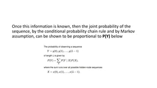
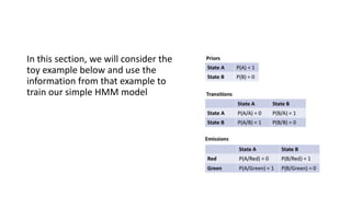
Hidden Markov models (HMMs) are probabilistic graphical models that allow prediction of a sequence of hidden states from observed variables. HMMs make the Markov assumption that the next state depends only on the current state, not past states. They require specification of transition probabilities between hidden states, emission probabilities of observations given states, and initial state probabilities to compute the joint probability of state sequences given observations. The most probable hidden state sequence, determined from these probabilities, is taken as the best inference.

1. Hidden Markov Models

2. Introduction
An HMM can be viewed as a Bayes Net unrolled through time with
observations made at a sequence of time steps being used to predict
the best sequence of hidden states.

3. Statement
Hidden Markov Models (HMMs) are a class of probabilistic graphical
model that allow us to predict a sequence of unknown (hidden)
variables from a set of observed variables.

4. Explanation
The reason it is called a Hidden Markov Model is because we are
constructing an inference model based on the assumptions of a Markov
process. The Markov process assumption is simply that the “future is
independent of the past given the present”. In other words, assuming
we know our present state, we do not need any other historical
information to predict the future state.

5. Example
To make this point clear, let us consider the scenario below where the
weather, the hidden variable, can be hot, mild or cold and the observed
variables are the type of clothing worn. The arrows represent
transitions from a hidden state to another hidden state or from a
hidden state to an observed variable.
Notice that, true to the Markov assumption, each state only depends
on the previous state and not on any other prior states.

7. Advantages
HMMs are probabilistic models. They allow us to compute the joint
probability of a set of hidden states given a set of observed states. The
hidden states are also referred to as latent states. Once we know the
joint probability of a sequence of hidden states, we determine the best
possible sequence i.e. the sequence with the highest probability and
choose that sequence as the best sequence of hidden states.

8. Point to note
The ratio of hidden states to observed states is not necessarily 1 is to 1.
The key idea is that one or more observations allow us to make an
inference about a sequence of hidden states.
In order to compute the joint probability of a sequence of hidden
states, we need to assemble three types of information.

9. States
Generally, the term “states” are used to refer to the hidden states and
“observations” are used to refer to the observed states.
Transition data— the probability of transitioning to a new state
conditioned on a present state.
Emission data— the probability of transitioning to an observed state
conditioned on a hidden state.
Initial state information— the initial probability of transitioning to a
hidden state. This can also be looked at as the prior probability.

10. The above information can be computed directly from our training
data. For example, in the case of our weather example in Figure 1, our
training data would consist of the hidden state and observations for a
number of days. We could build our transition matrices of transitions,
emissions and initial state probabilities directly from this training data.

11. The example tables show a set of possible values that could be derived
for the weather/clothing scenario.

12. Once this information is known, then the joint probability of the
sequence, by the conditional probability chain rule and by Markov
assumption, can be shown to be proportional to P(Y) below

13. If there are k possible values for each hidden sequence and we have a
sequence length of n, there there are n^k total possible sequences that
must be all scored and ranked in order to determine a winning
candidate.

14. In this section, we will consider the
toy example below and use the
information from that example to
train our simple HMM model

15. In this example, we score a known sequence given some text
Let us consider the below sequence

16. • The score for this sequence can be computed as
The joint probability for our unknown sequence is therefore
P(A,B,A,Red,Green,Red) =
[P(y_0=A) P(x_0=Red/y_0=A)] [P(y_1=B|y_0=A|)
P(x_1=Green/y_1=B)] [P(y_2=A|y_1=B) P(x_2=Red/y_2=A)]
=(1∗1)∗(1∗0.75)∗(1∗1)(1)(1)=(1∗1)∗(1∗0.75)∗(1∗1)
=0.75(2)(2)=0.75