Downloaded 269 times


The document discusses gradient descent and its variants, focusing on how to optimize models through iterative adjustments of parameters using derivatives. It explains the concepts of forward and backpropagation in neural networks, highlighting the importance of applying the chain rule for calculating gradients. Additionally, it provides an overview of various optimization algorithms like stochastic gradient descent, momentum methods, and adaptive learning rates used in training neural networks.
Overview of backpropagation, gradient descent, and auto-differentiation by Sam Abrahams.
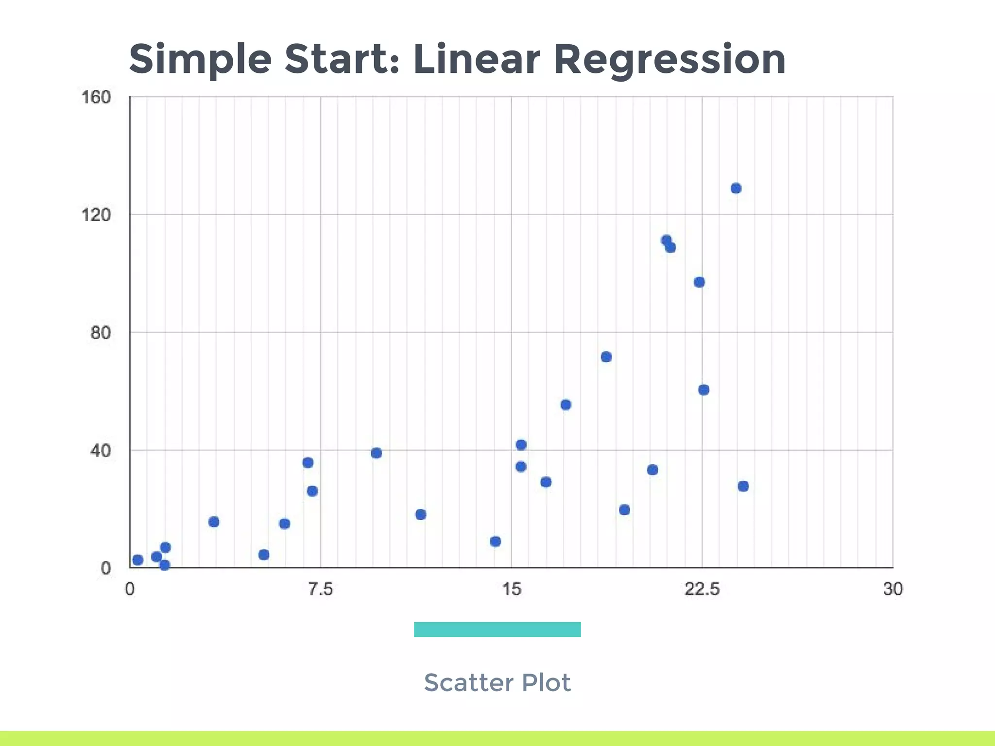
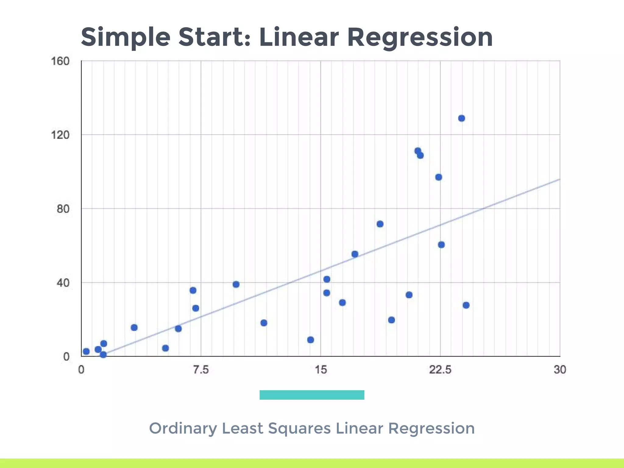
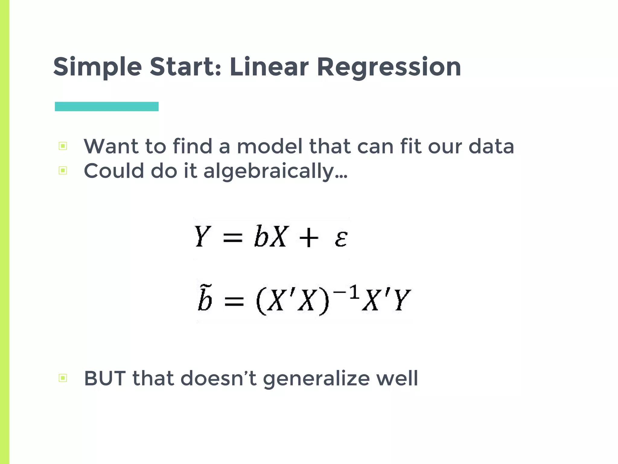
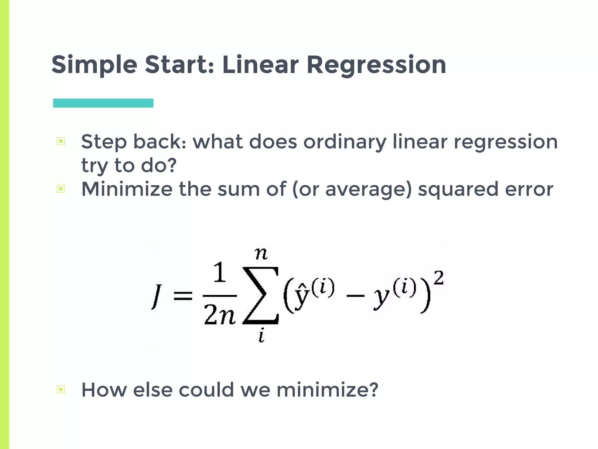
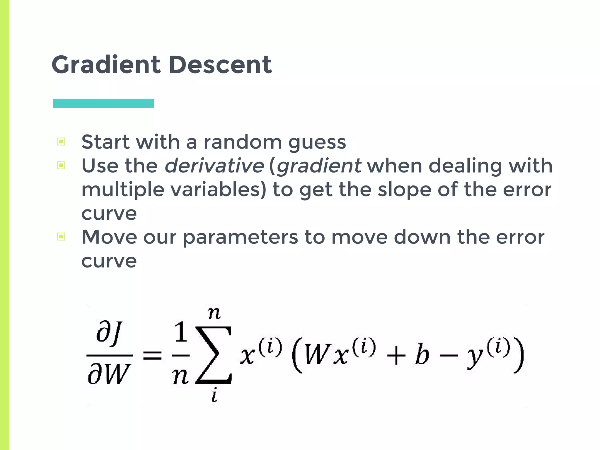
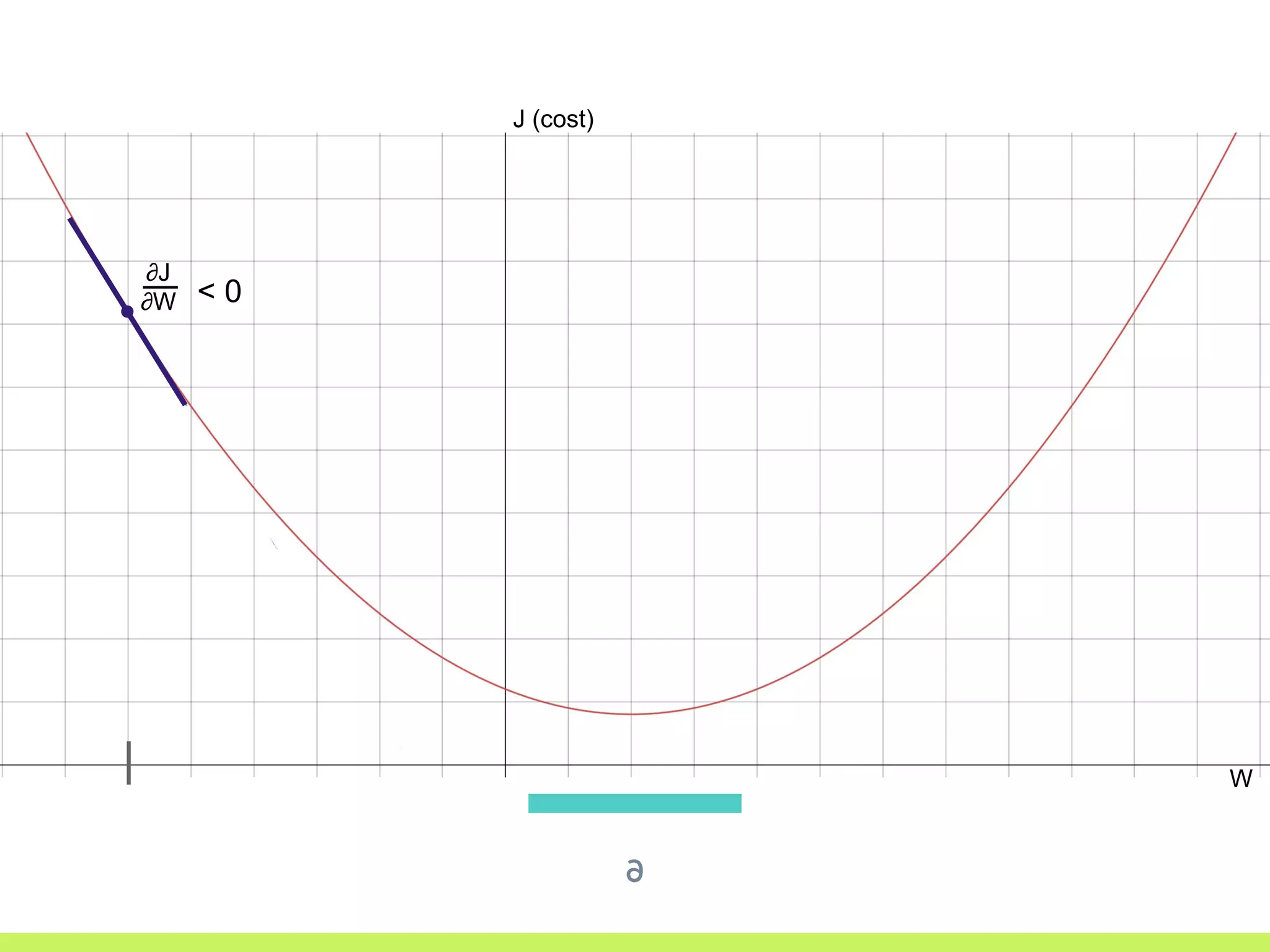
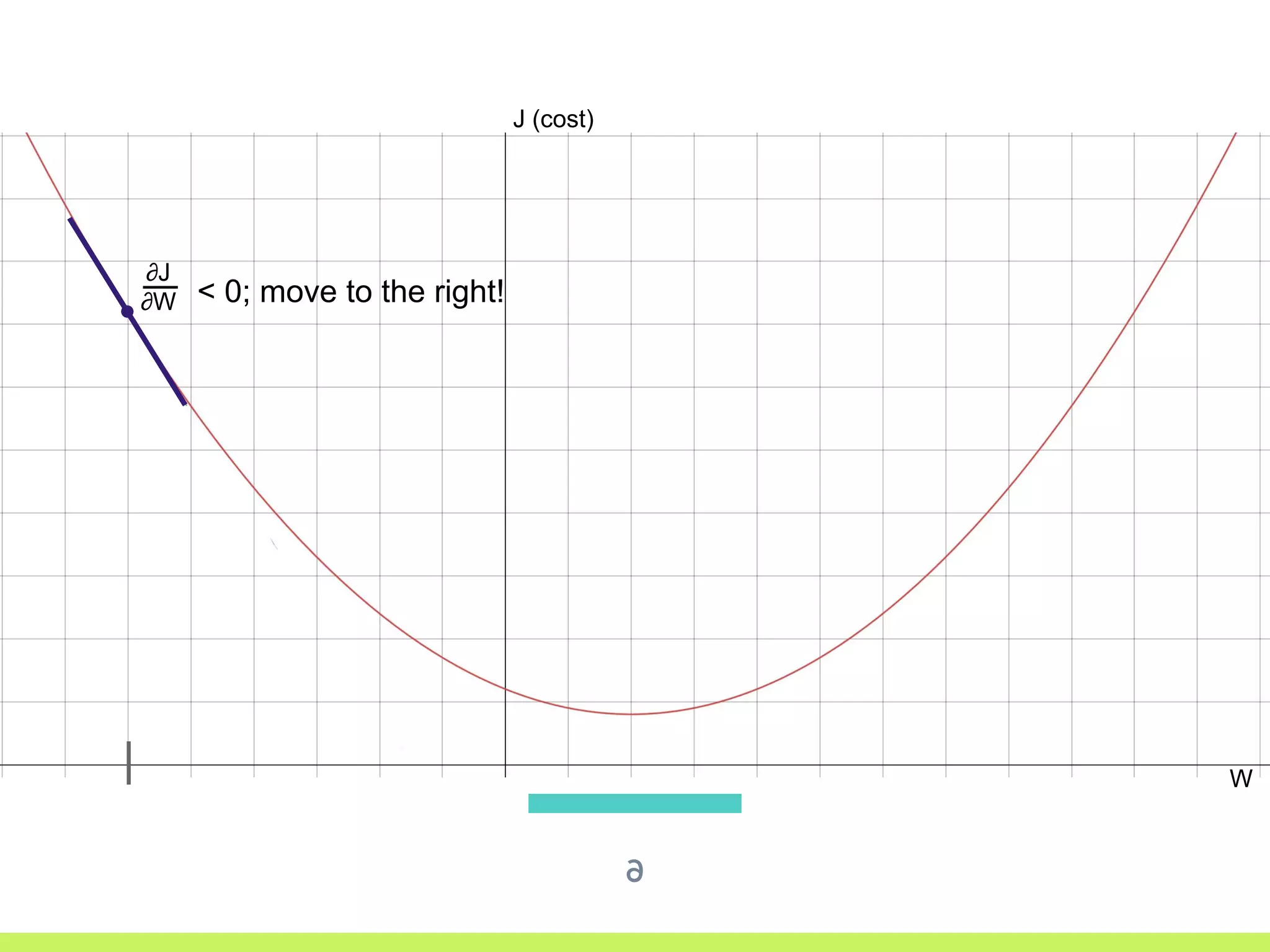
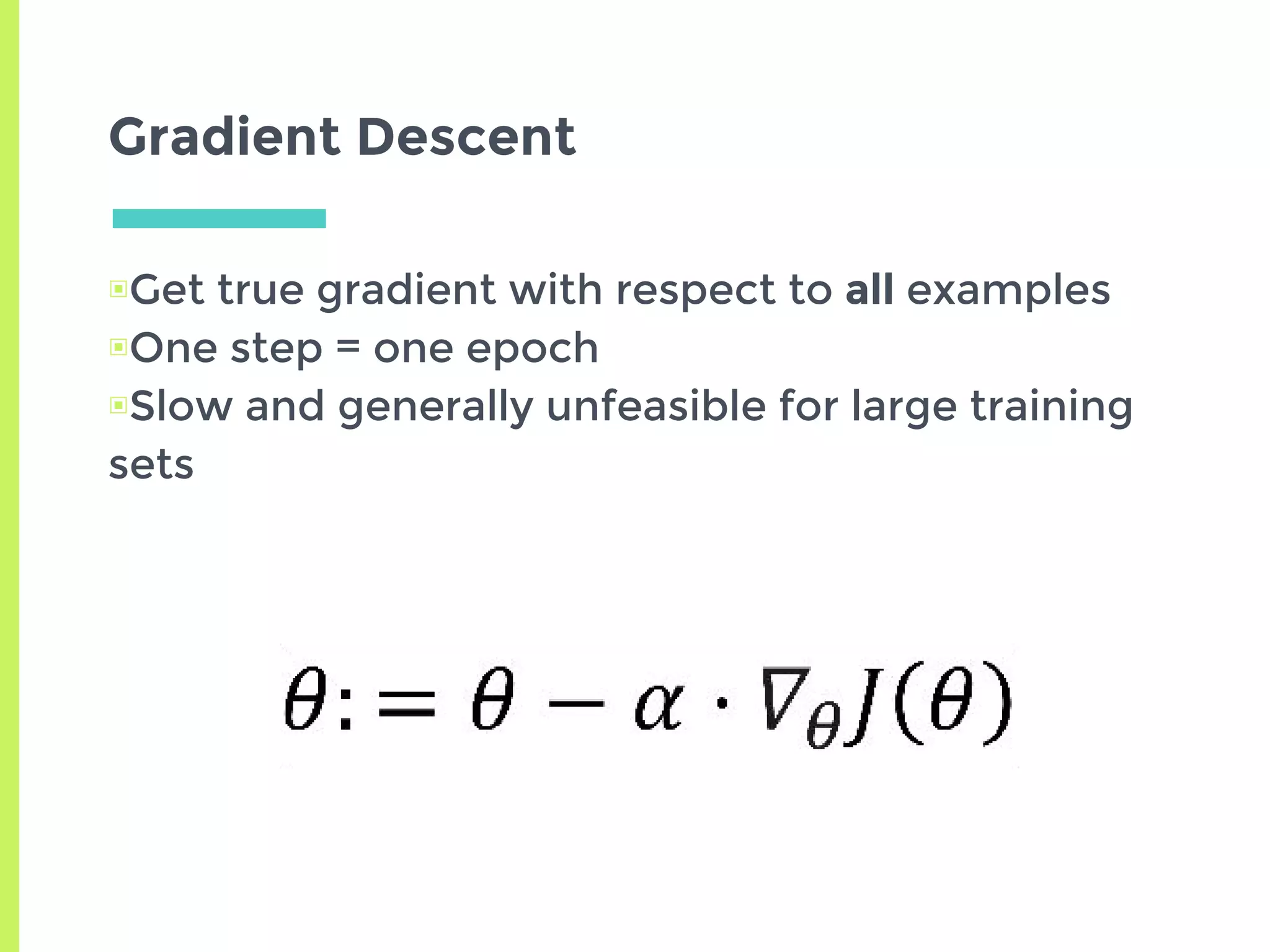
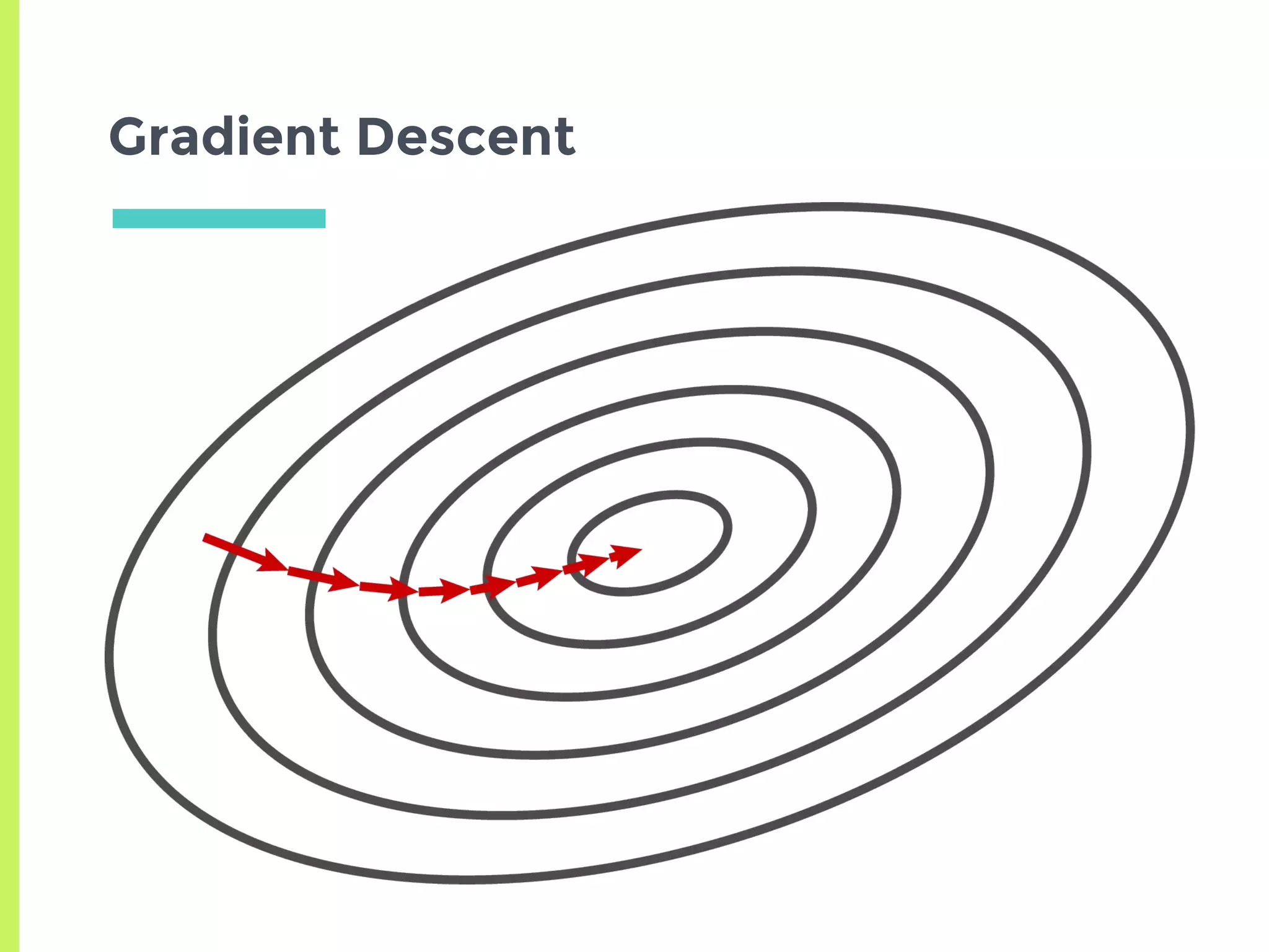
Introduction to Gradient Descent: fitting data using OLS, visualizing error curves, and an iterative approach to minimize error.
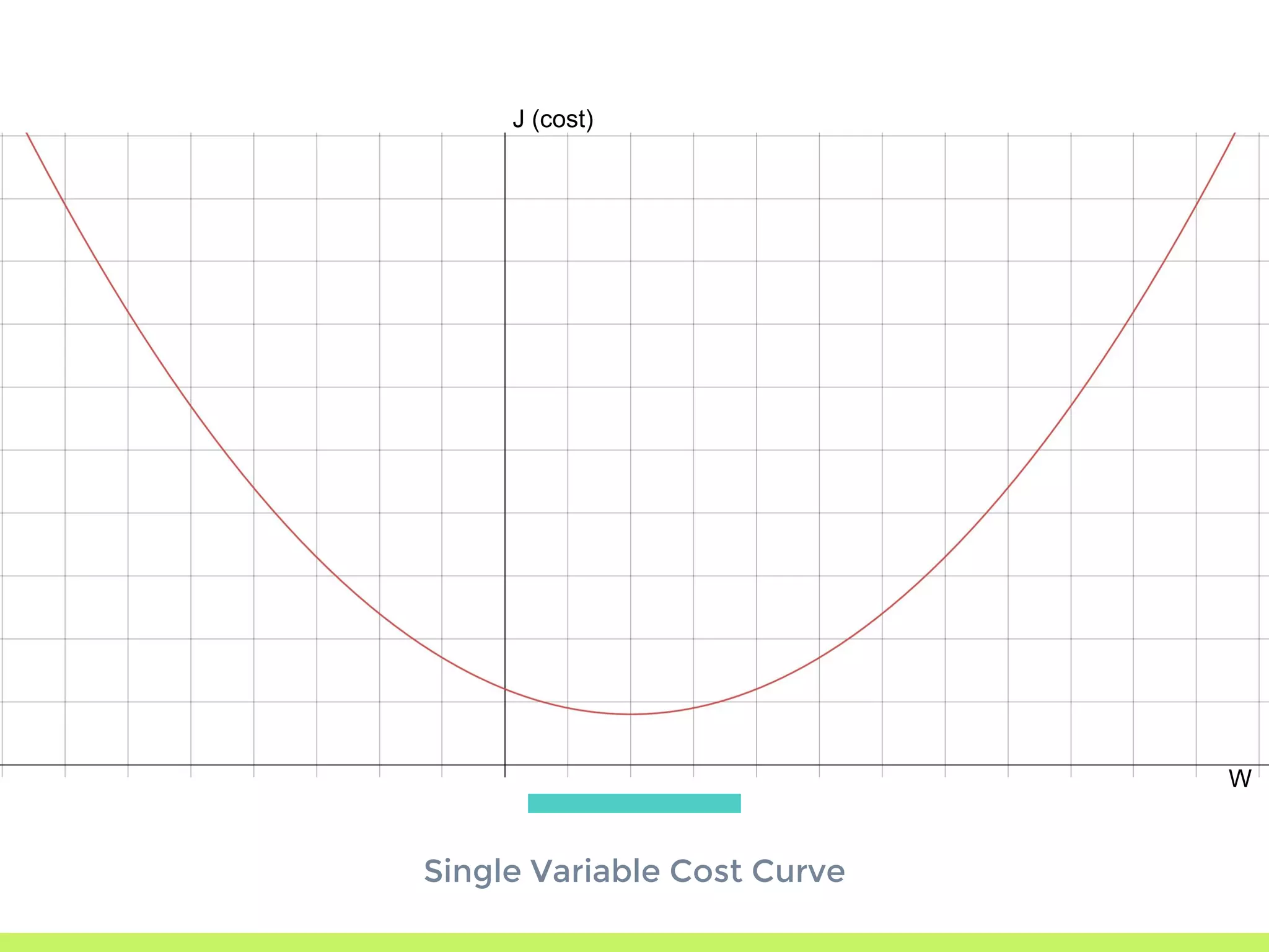
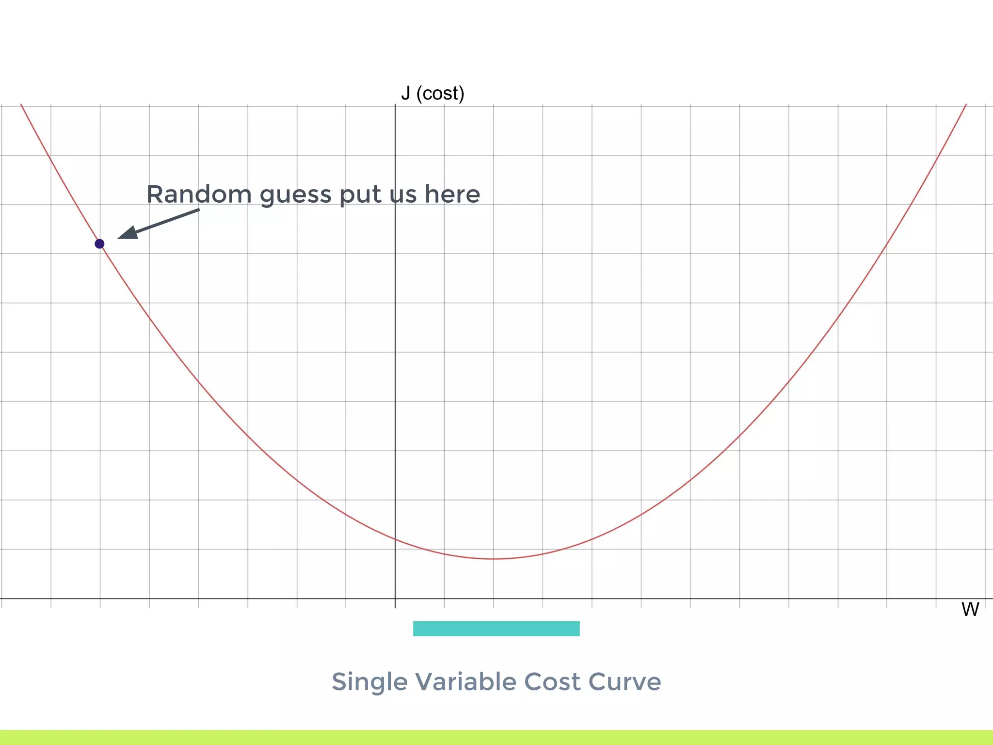
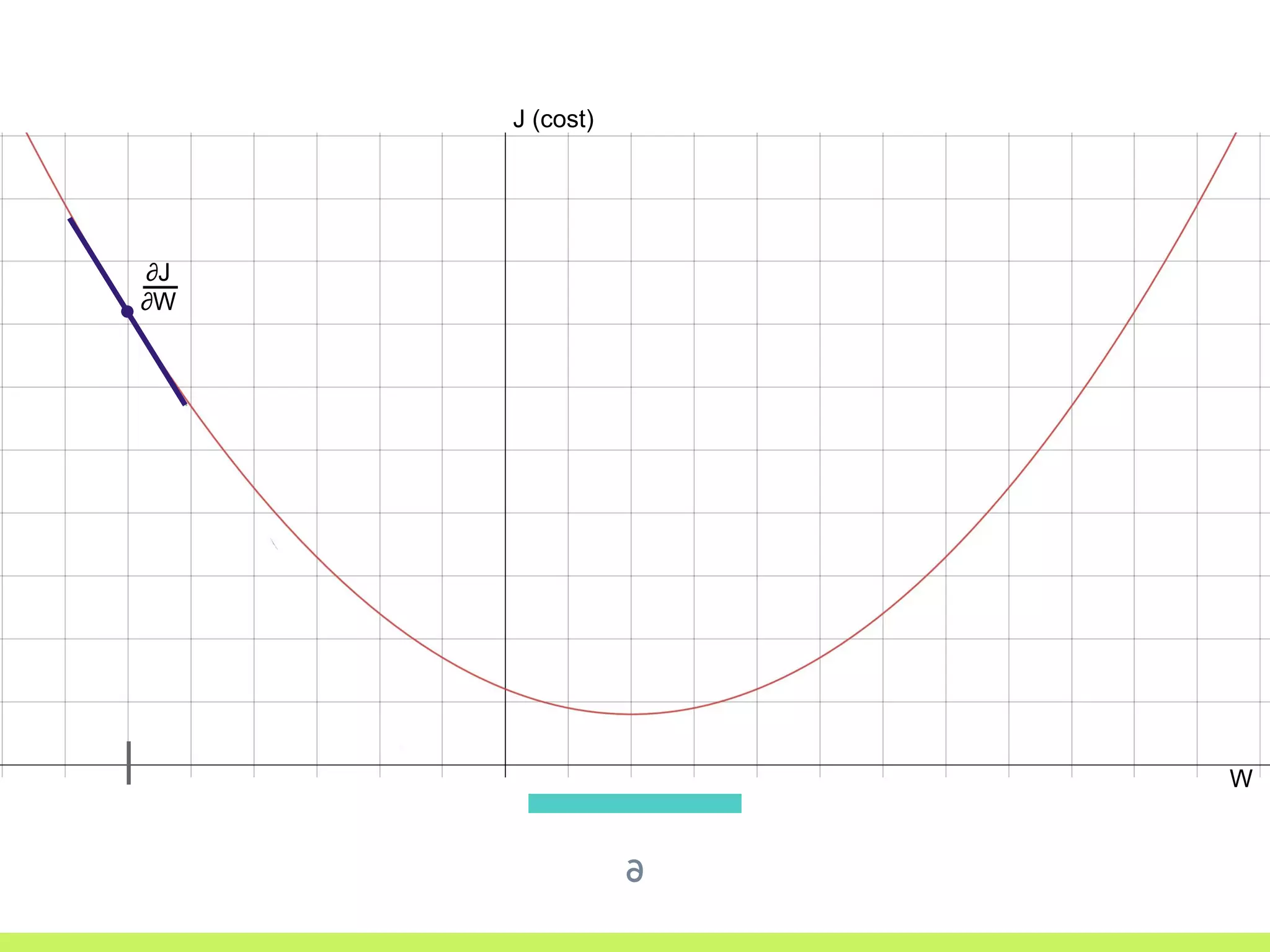
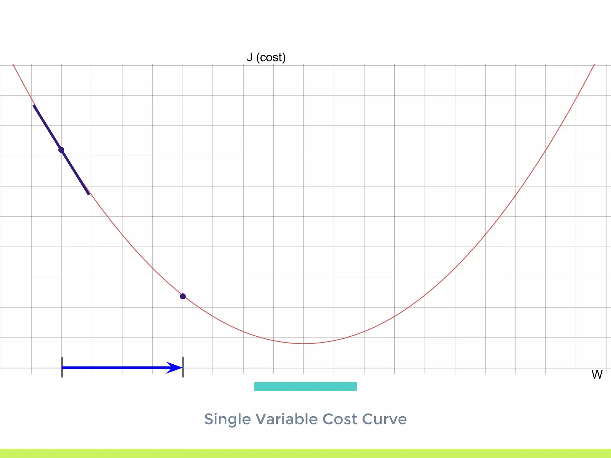
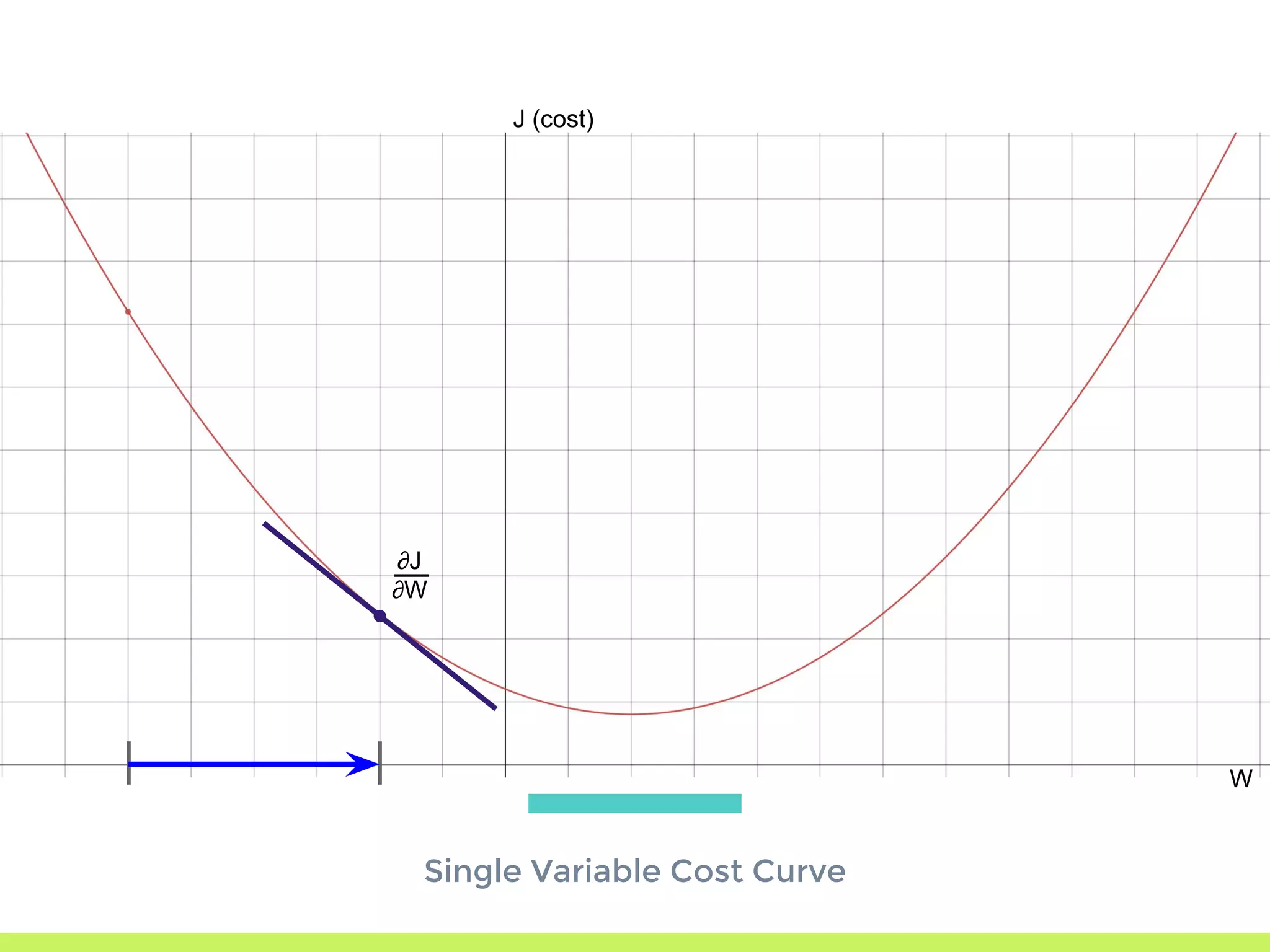
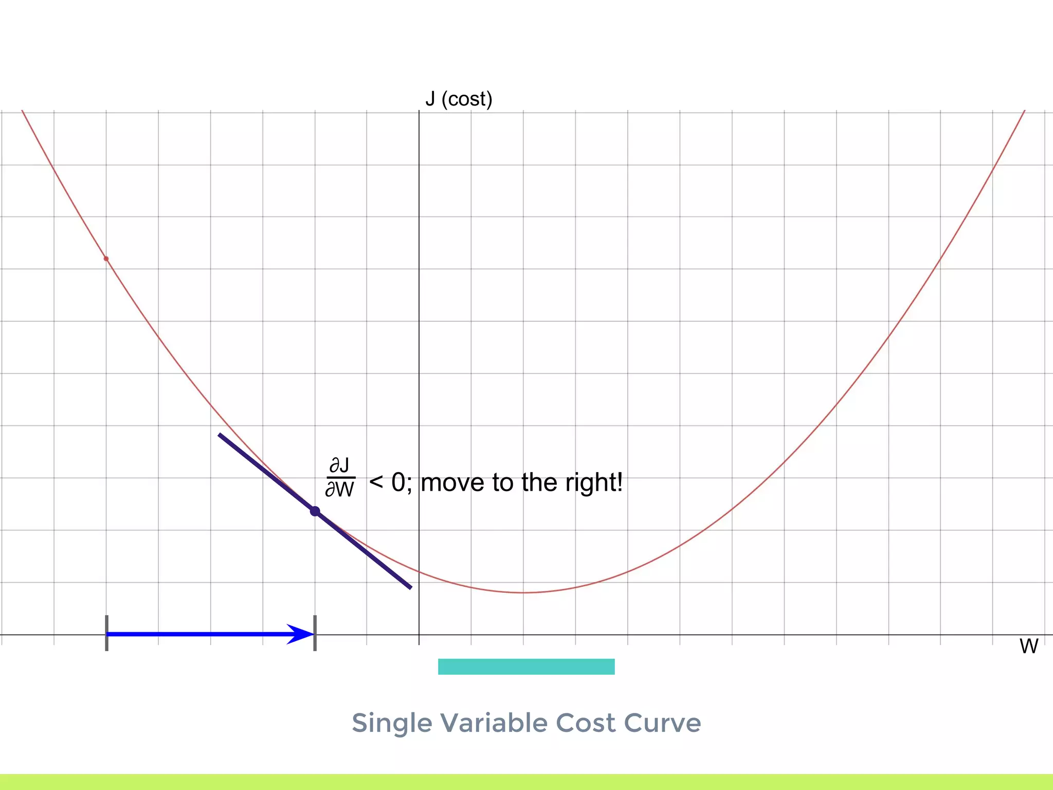
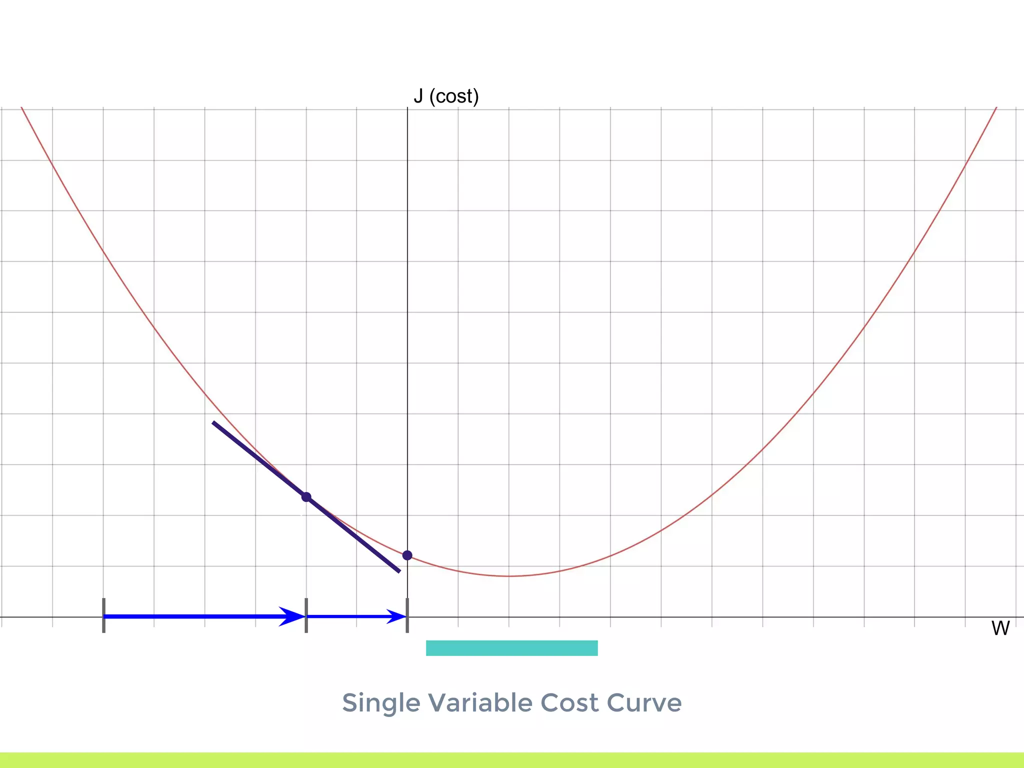
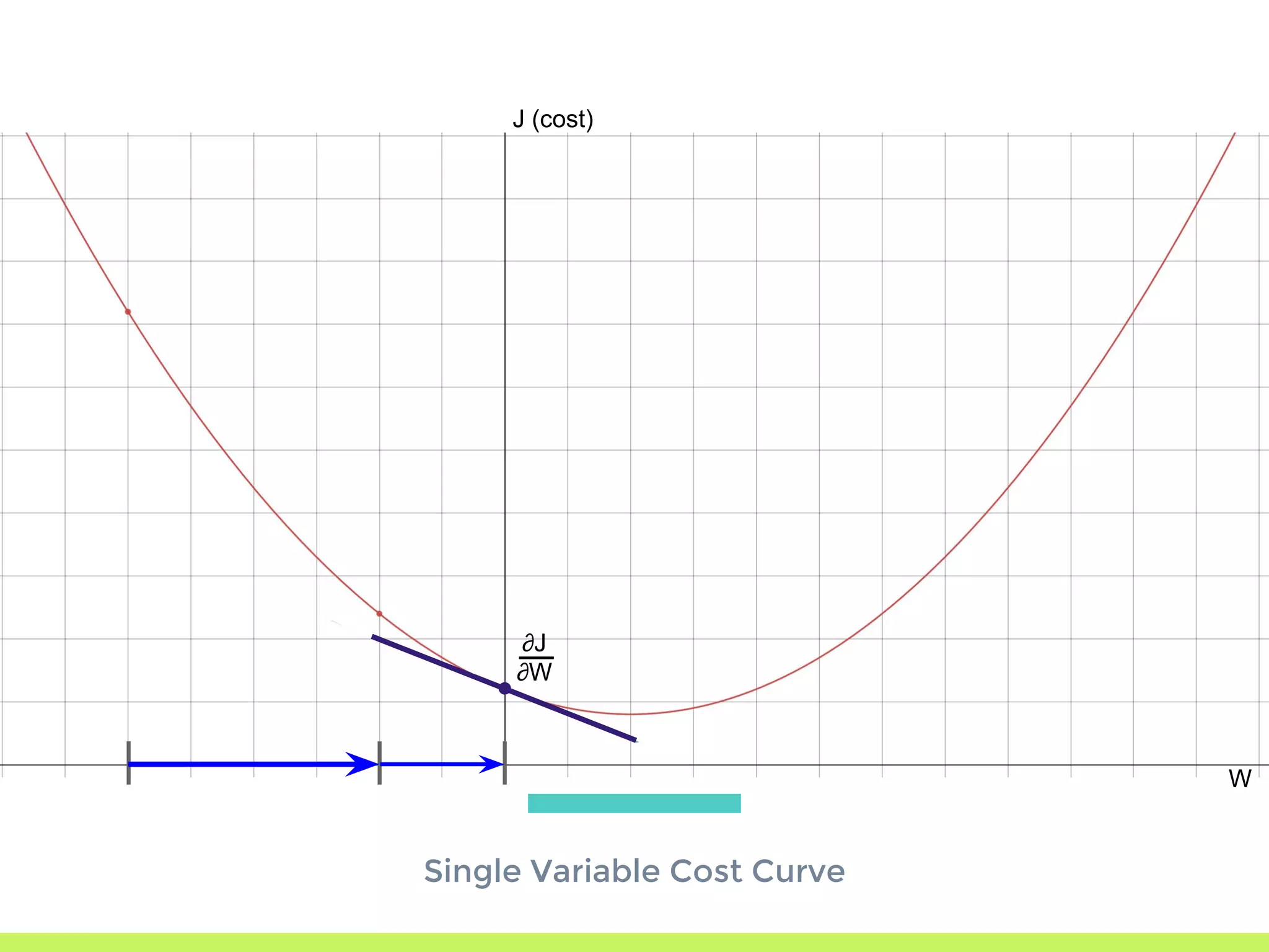
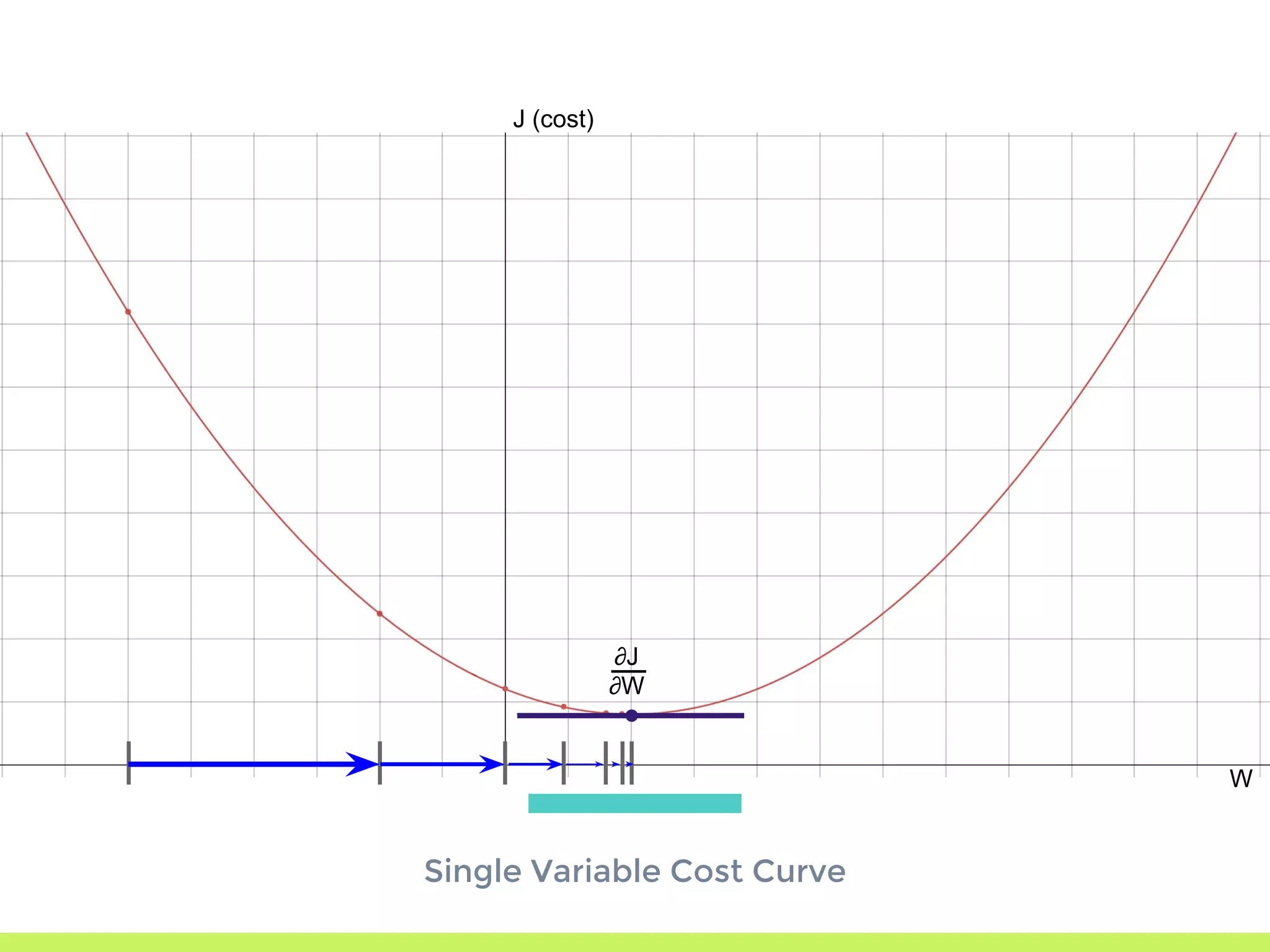
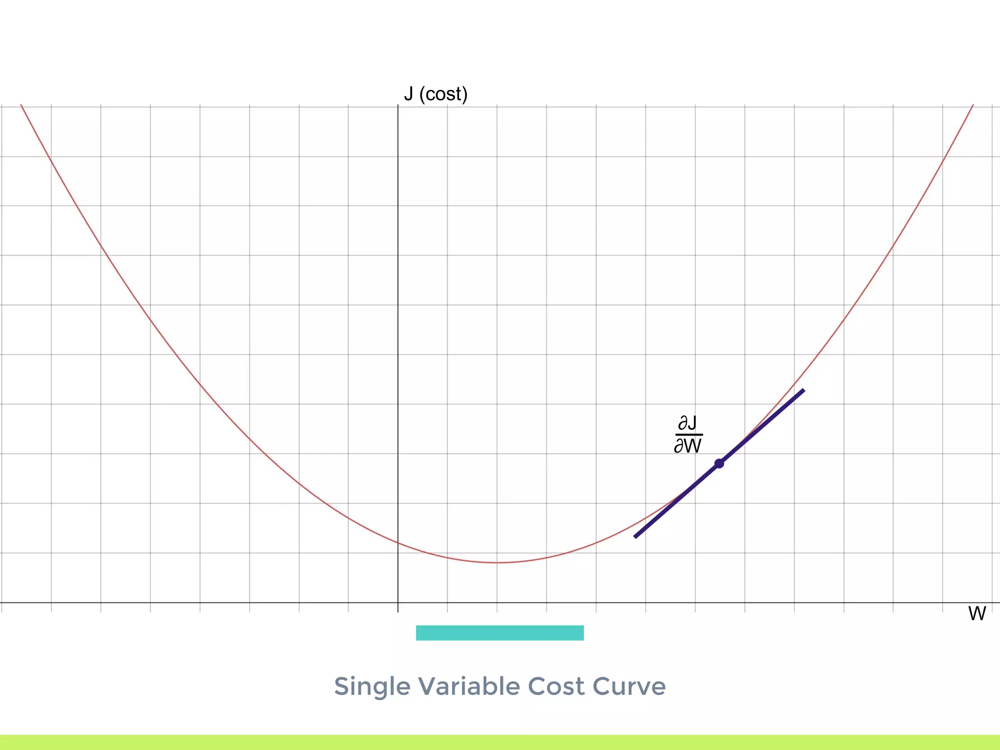
Single Variable Cost Curve: understanding the relationship between parameters, cost functions, and optimization through movement along the error curve.
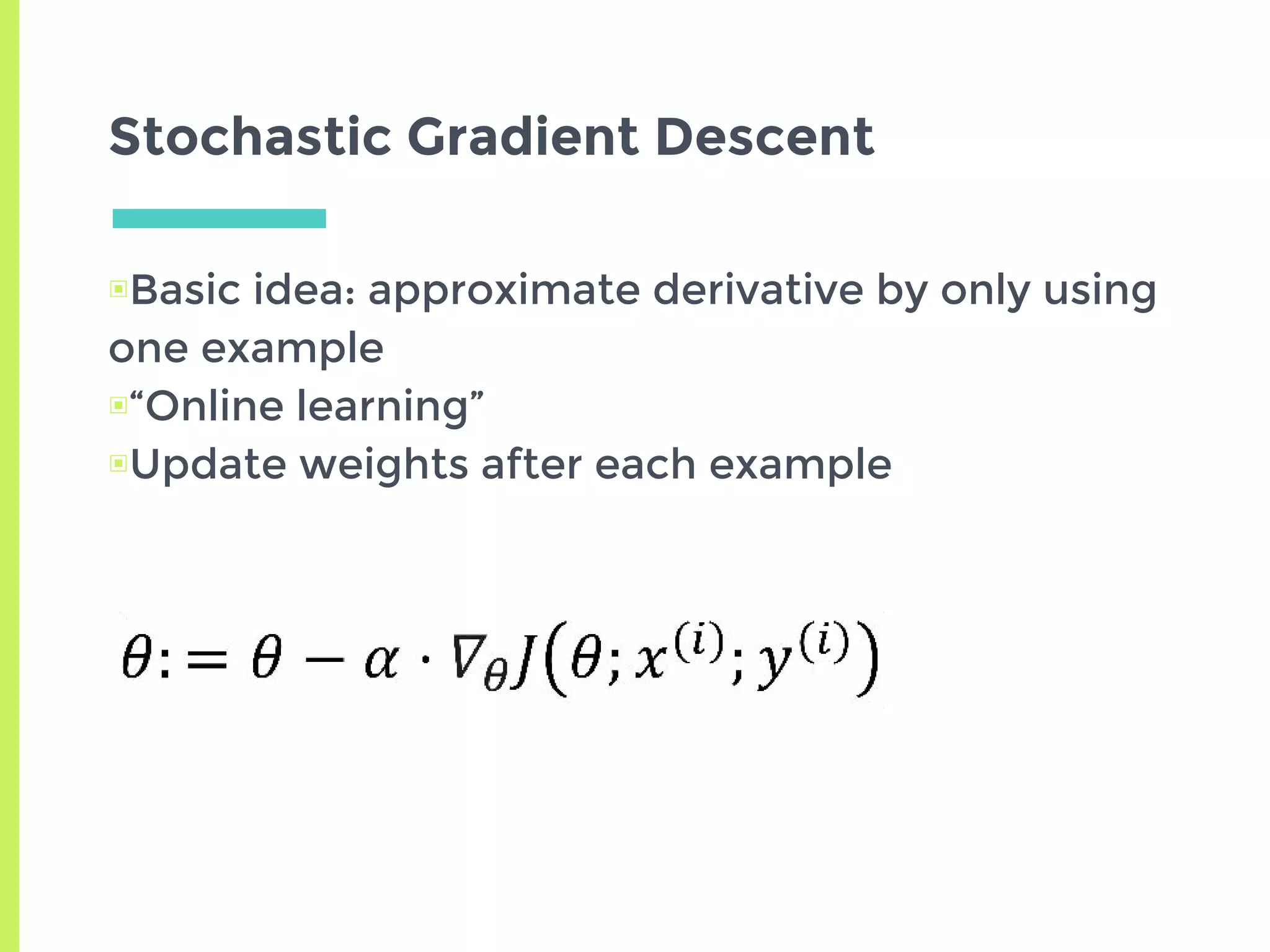
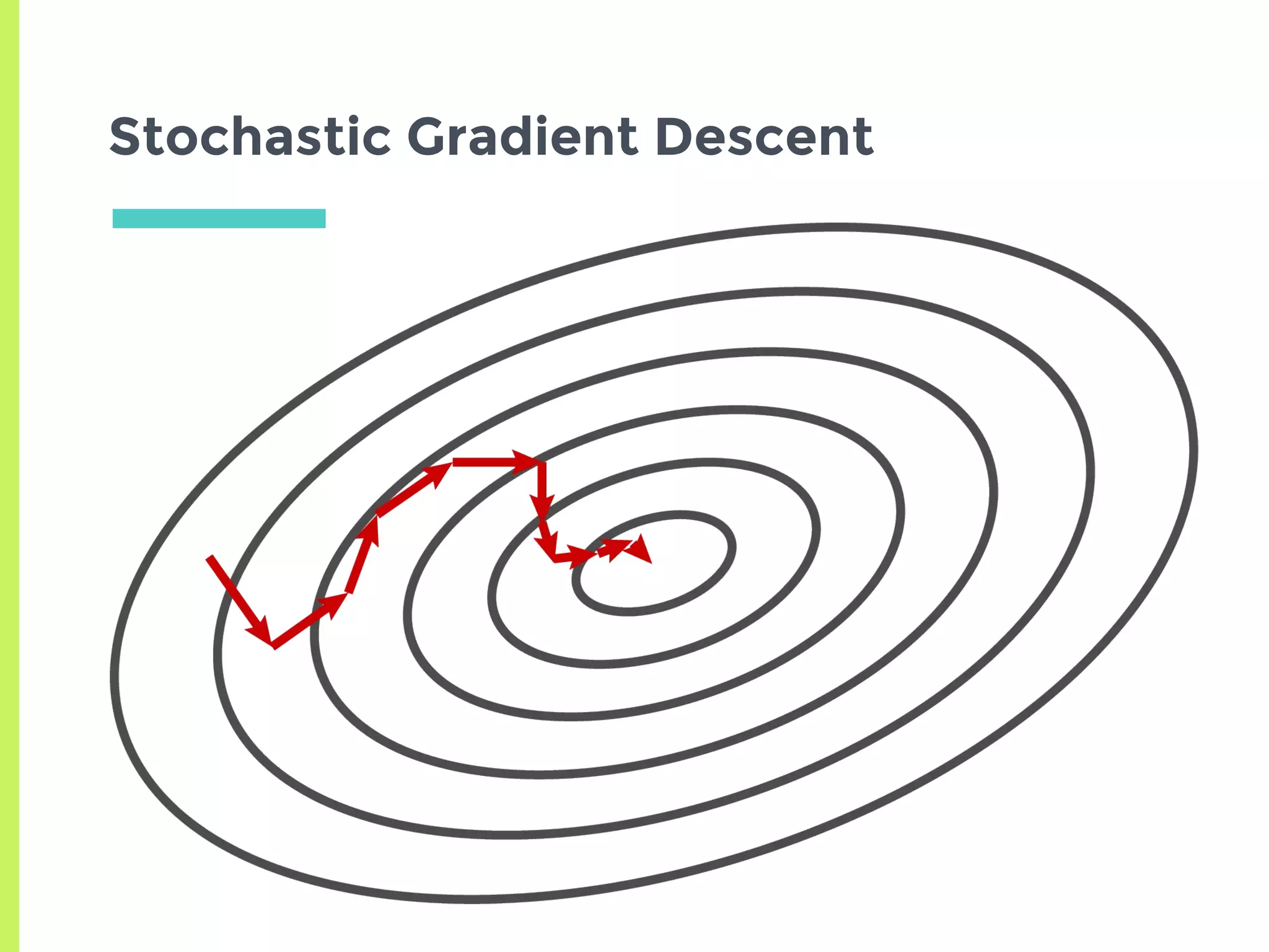
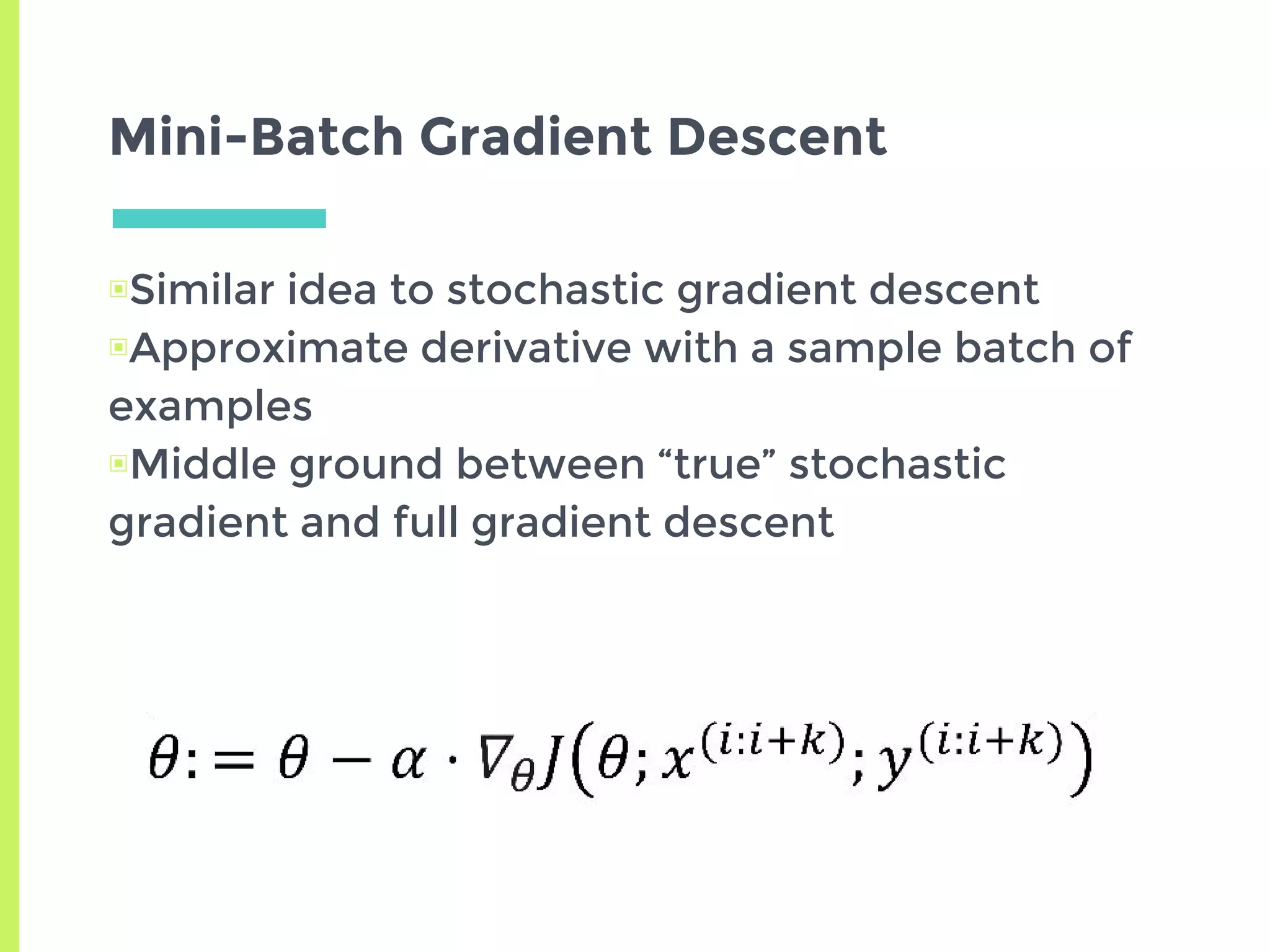
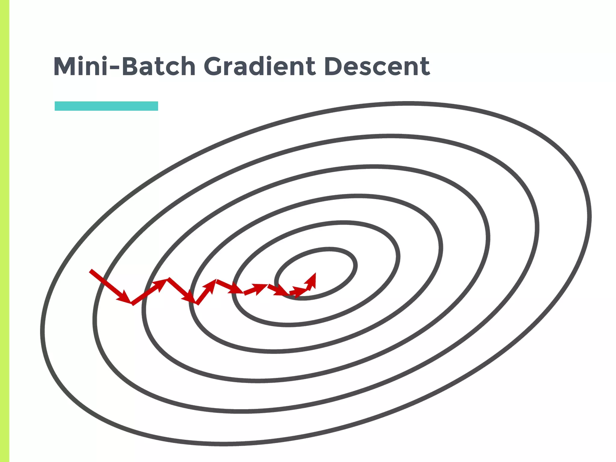
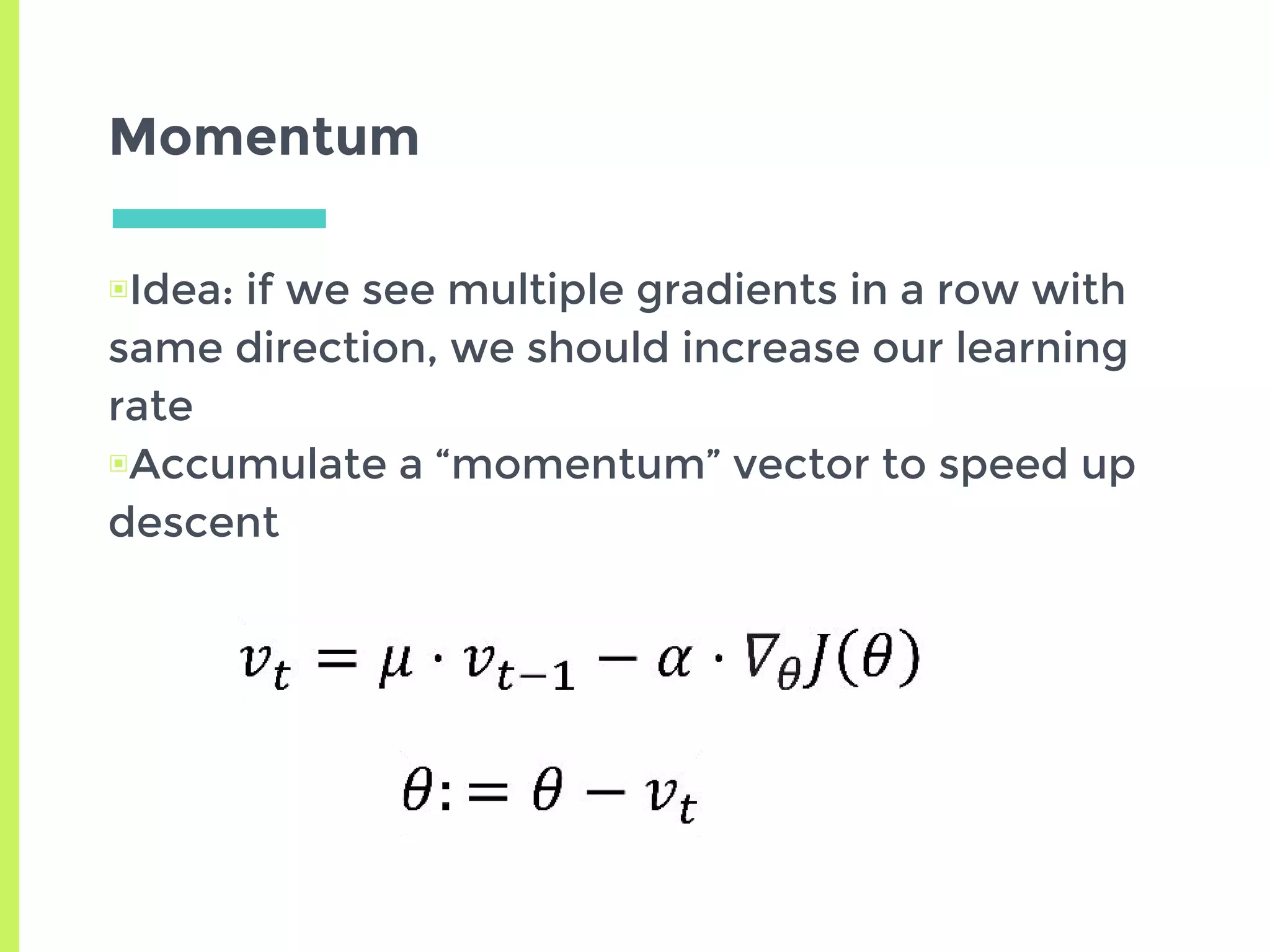
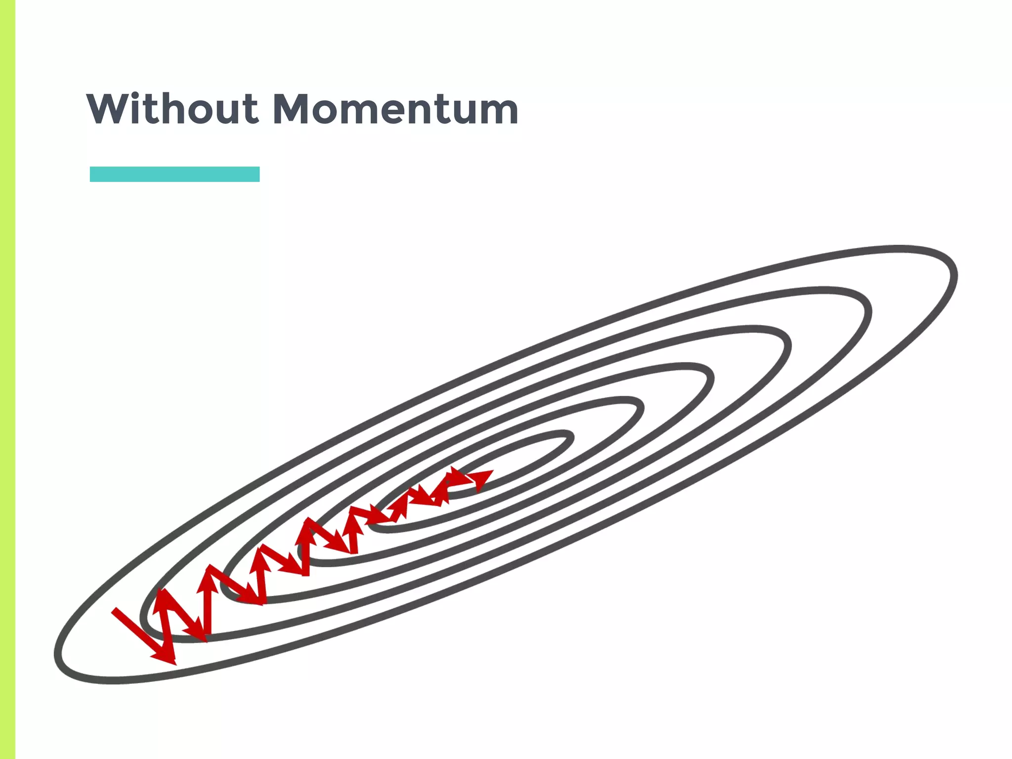
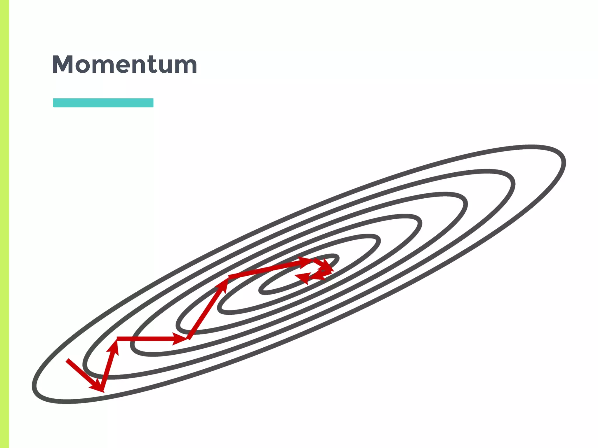
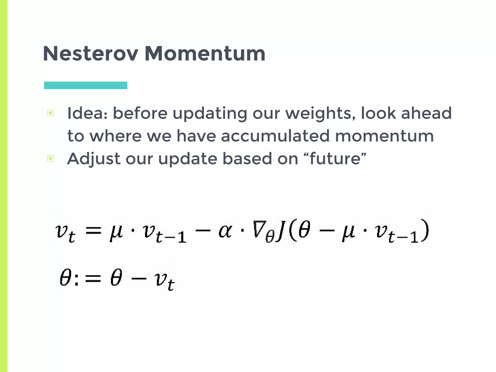
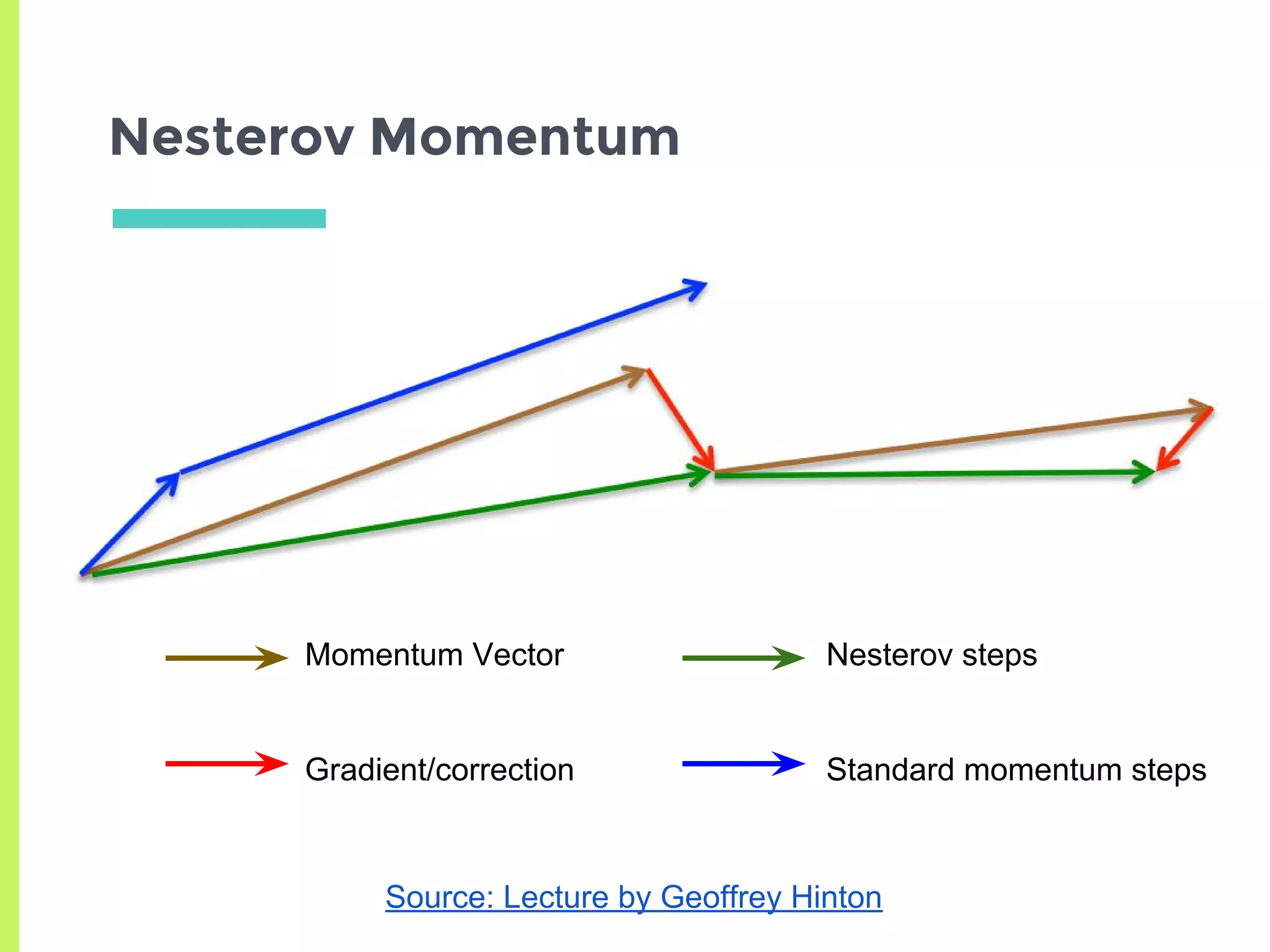
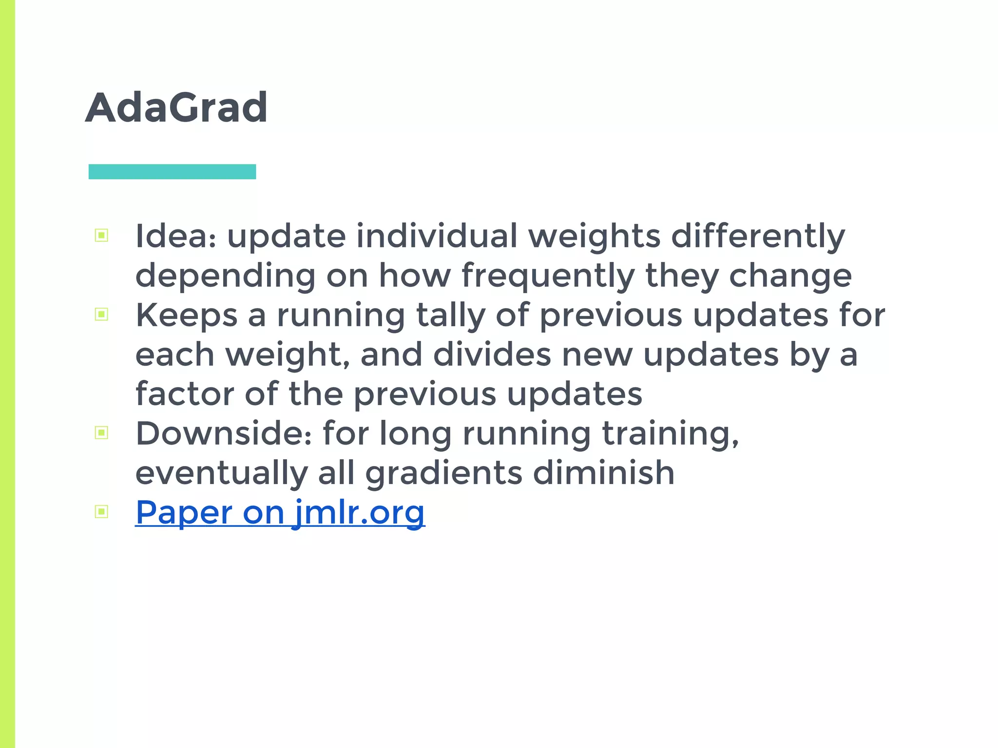
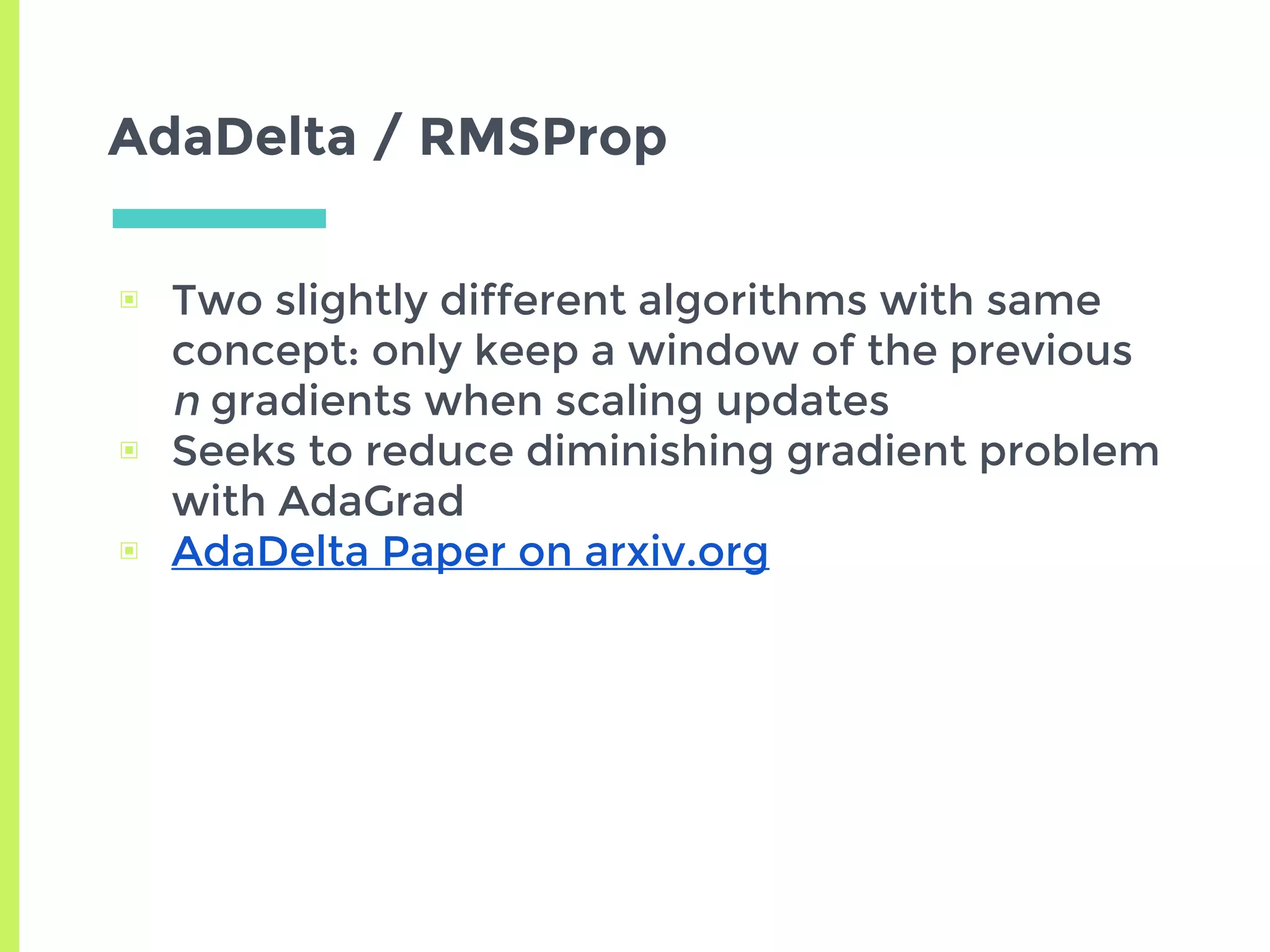
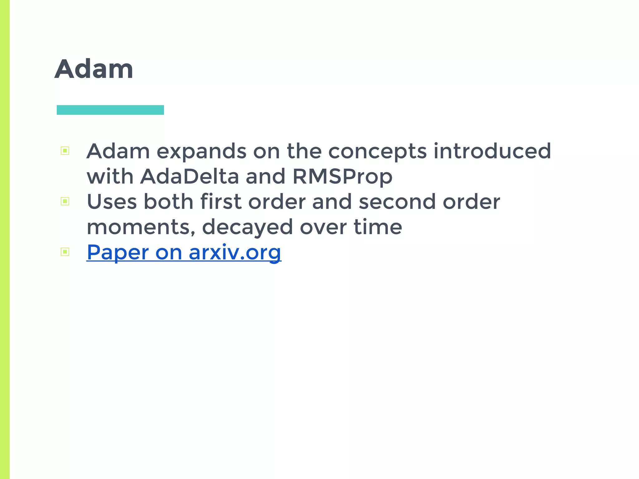
Exploration of variants of Gradient Descent including Stochastic, Mini-Batch, Momentum, and advanced methods like AdaGrad, RMSProp, and Adam.
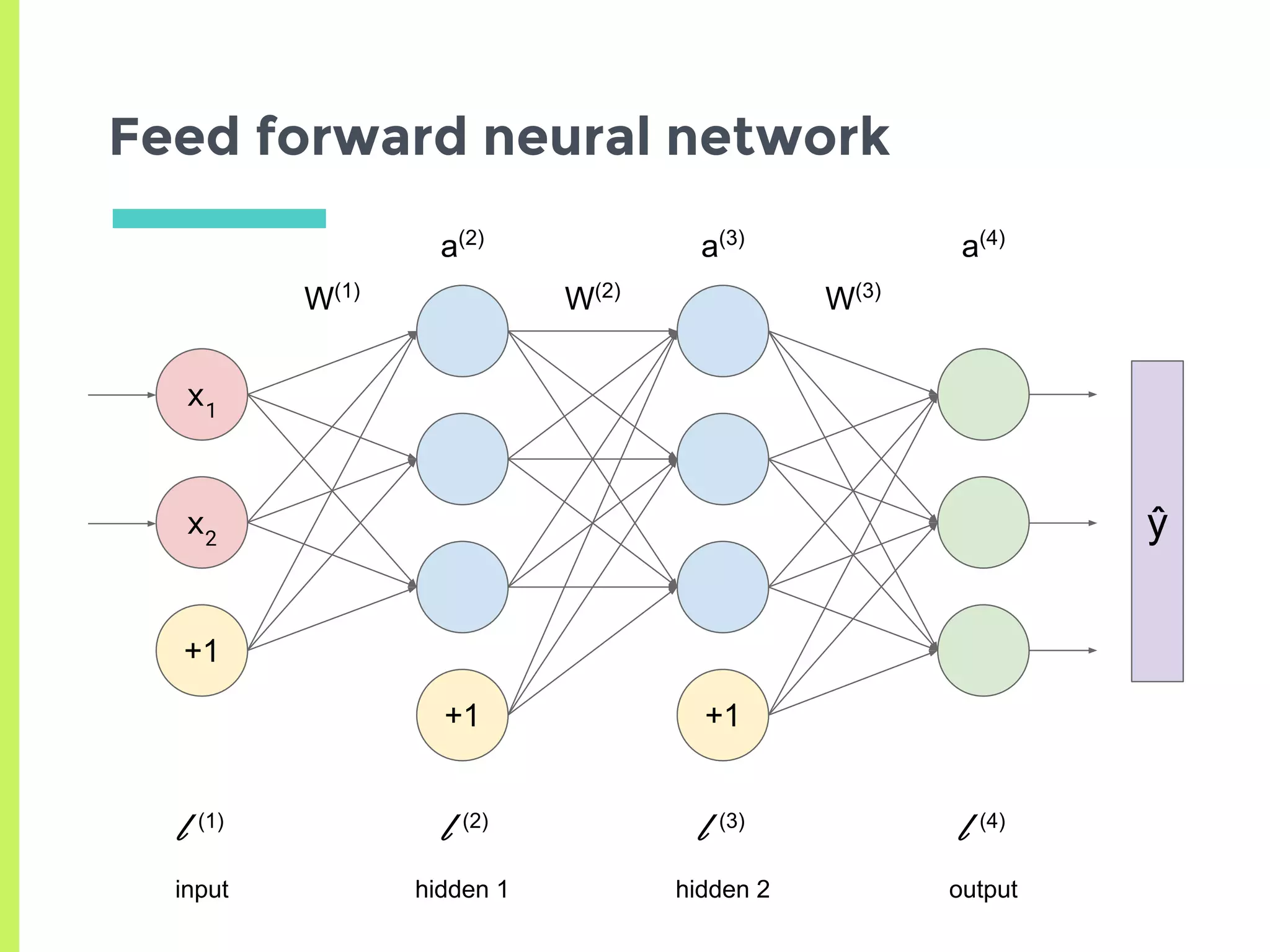
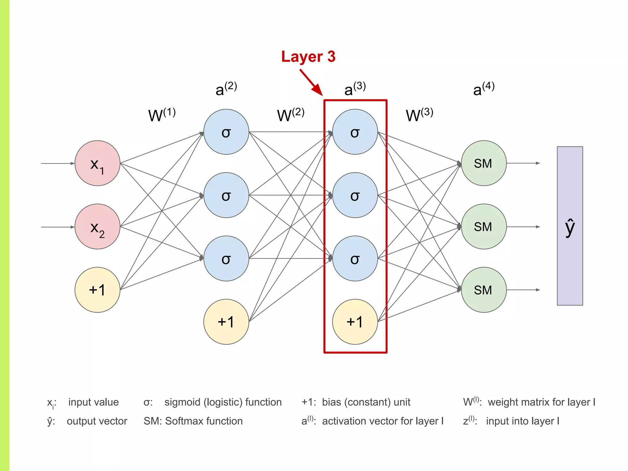
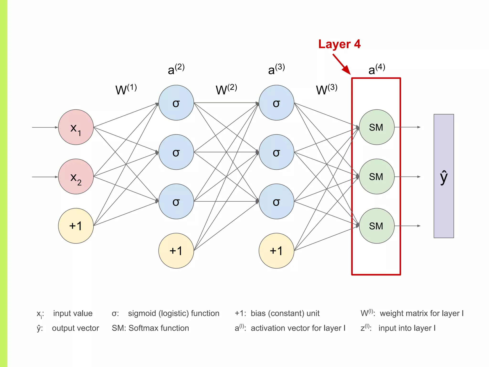
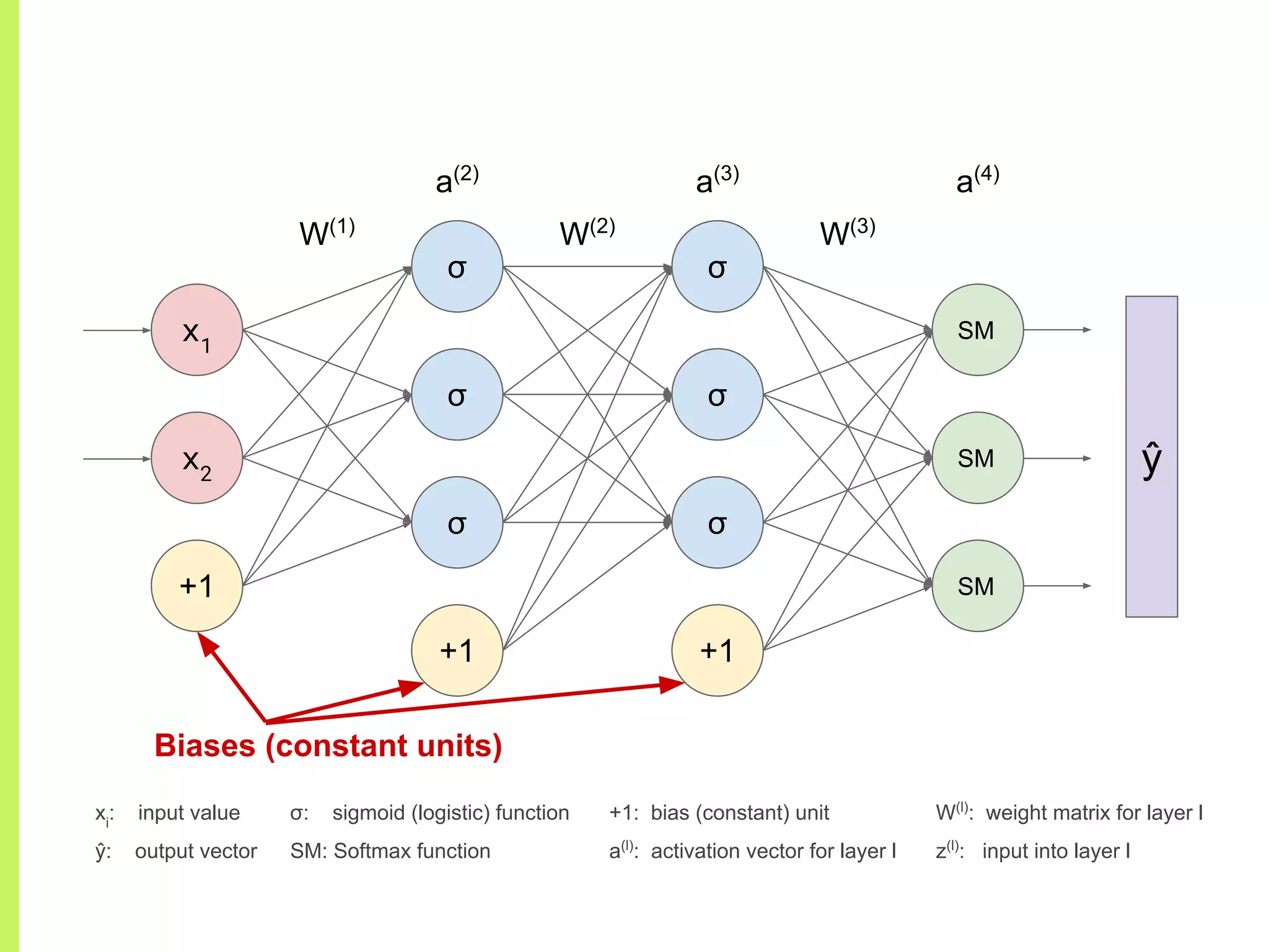
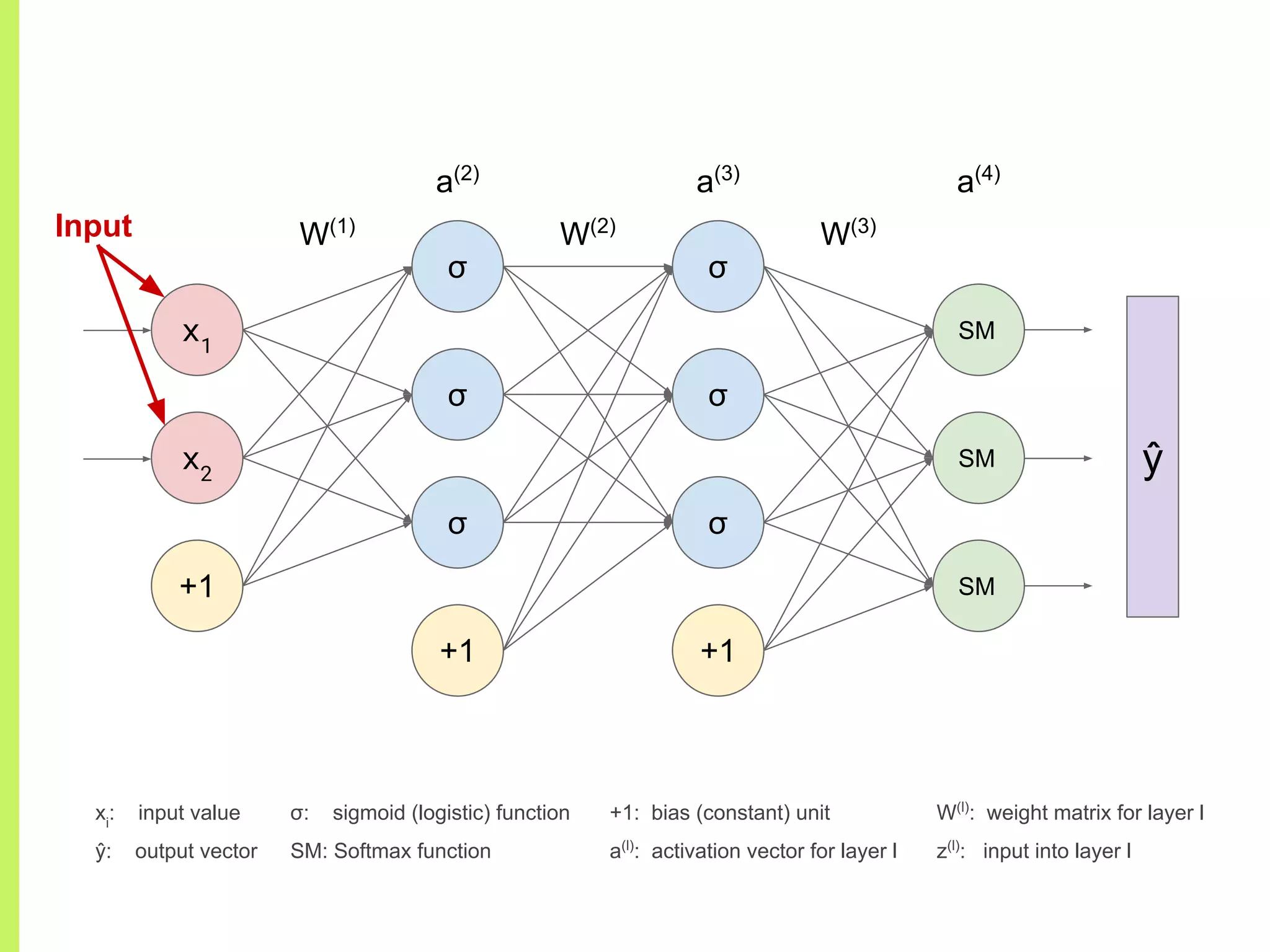
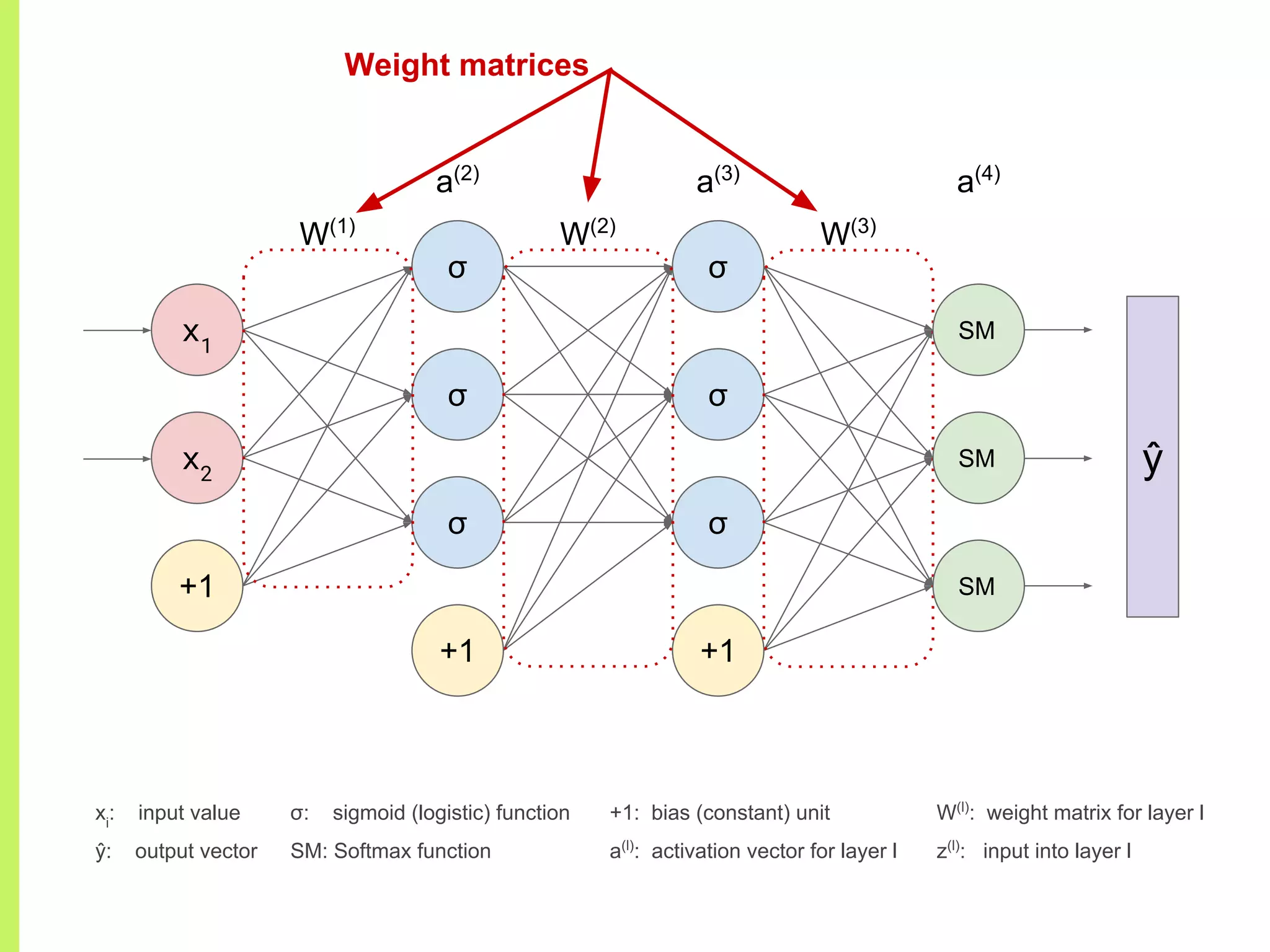
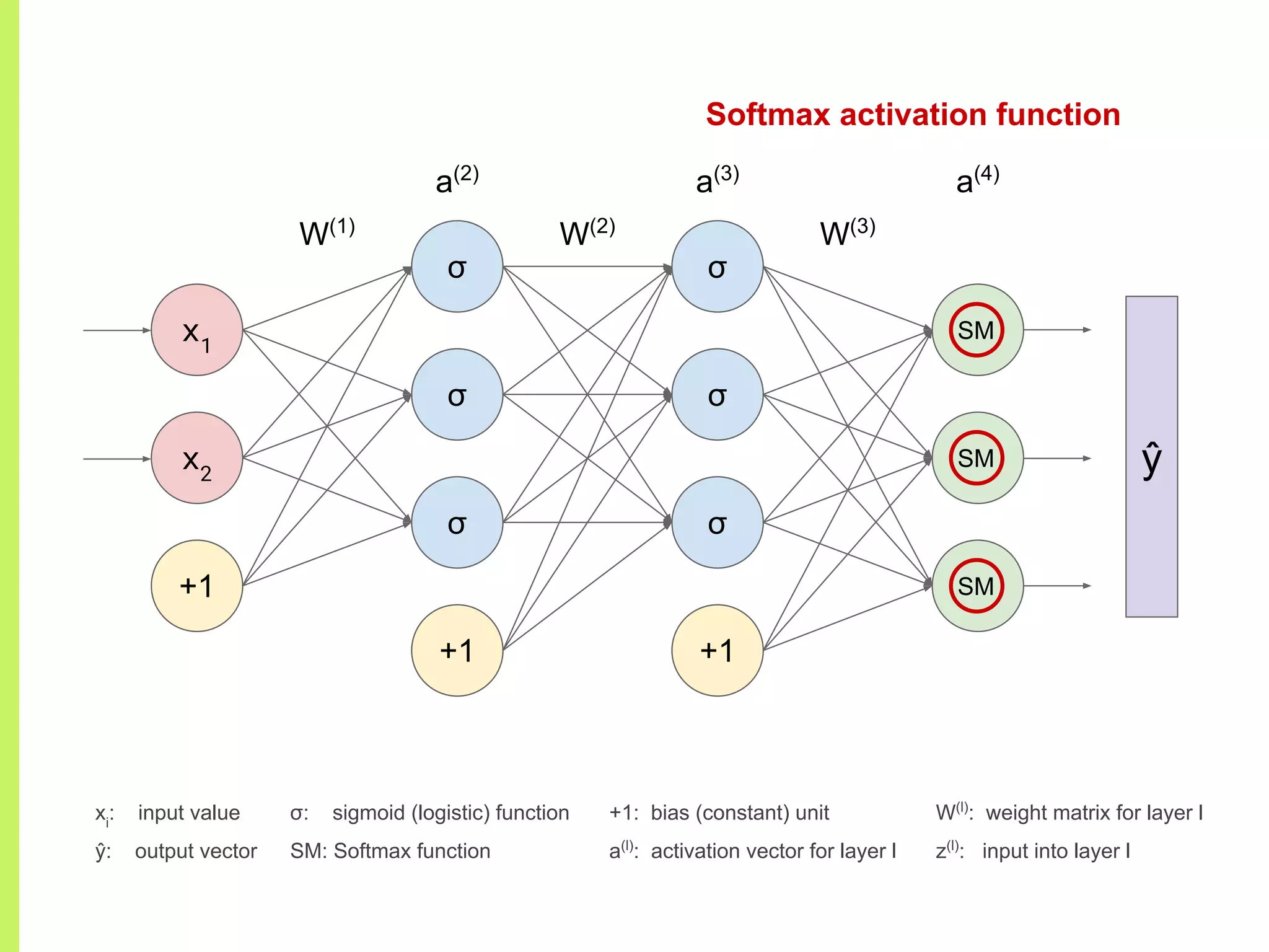
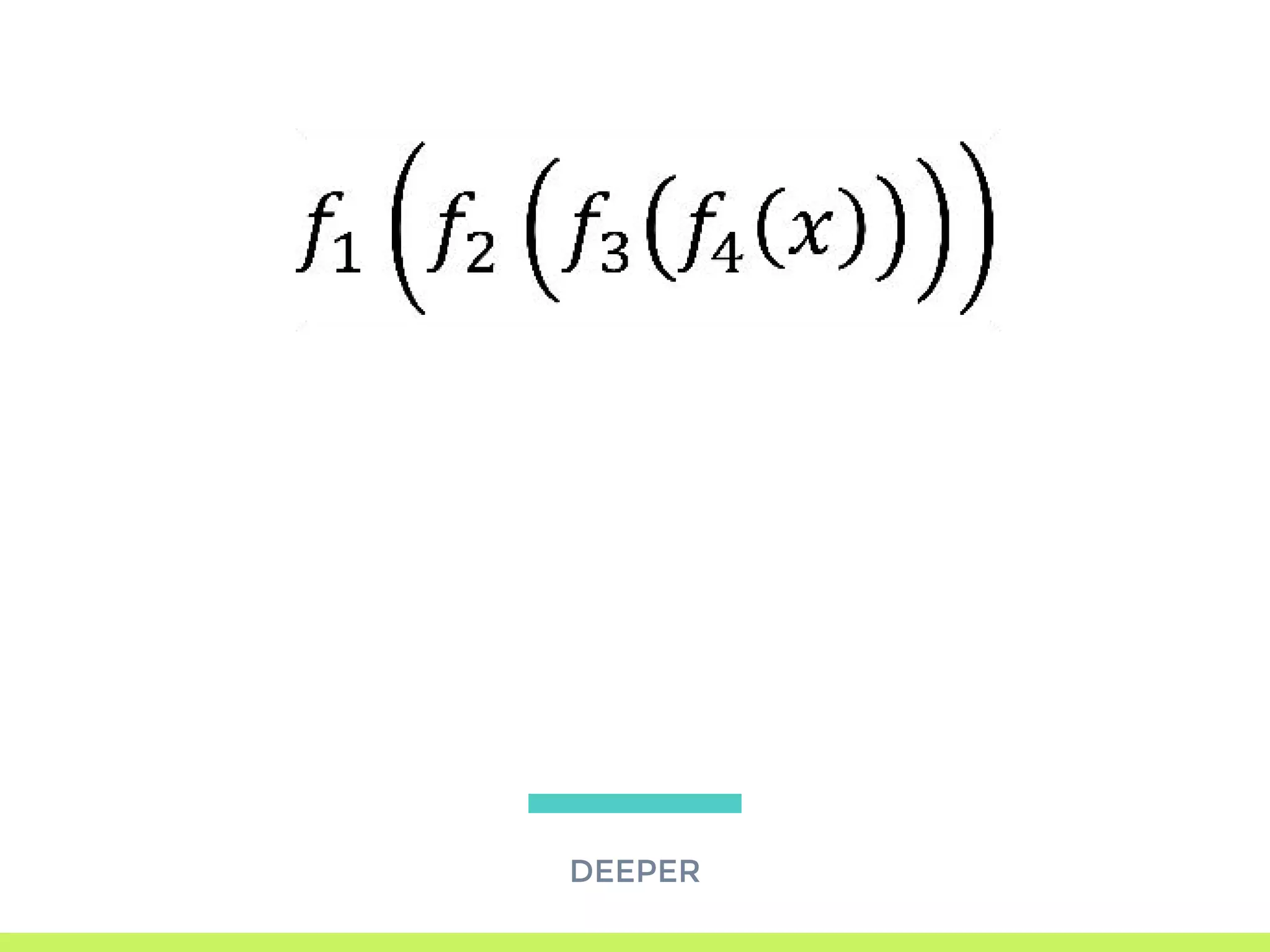
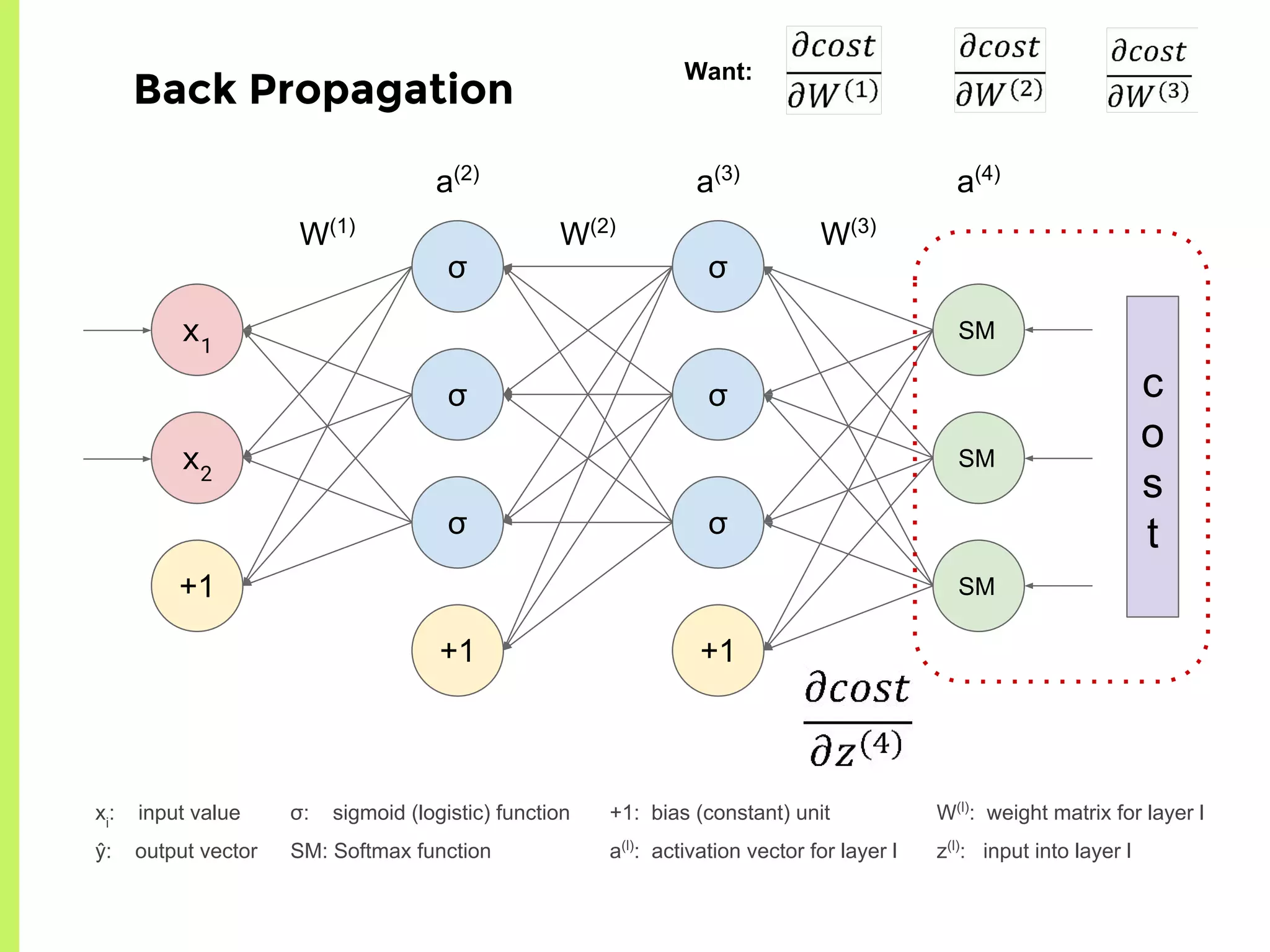
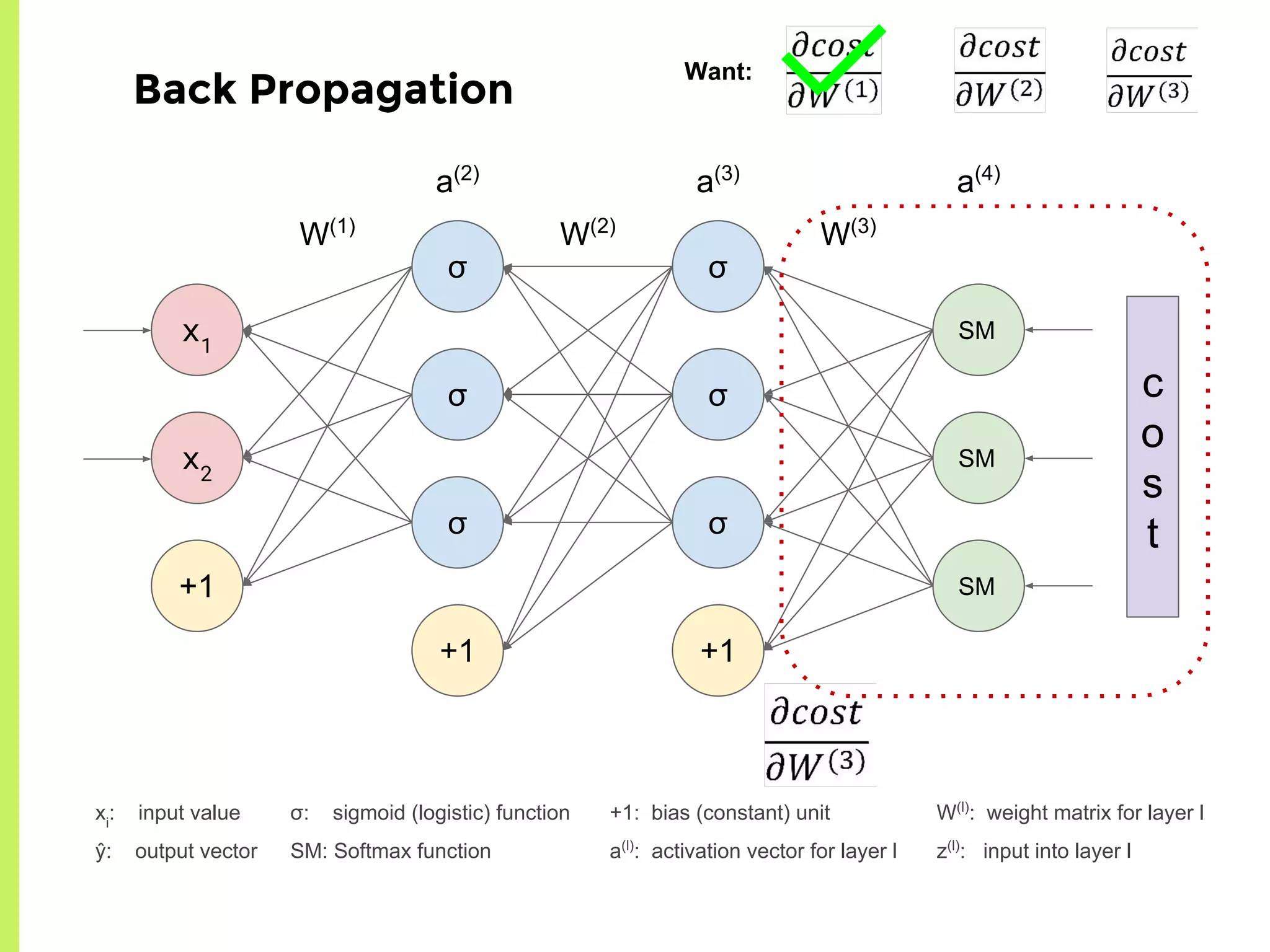
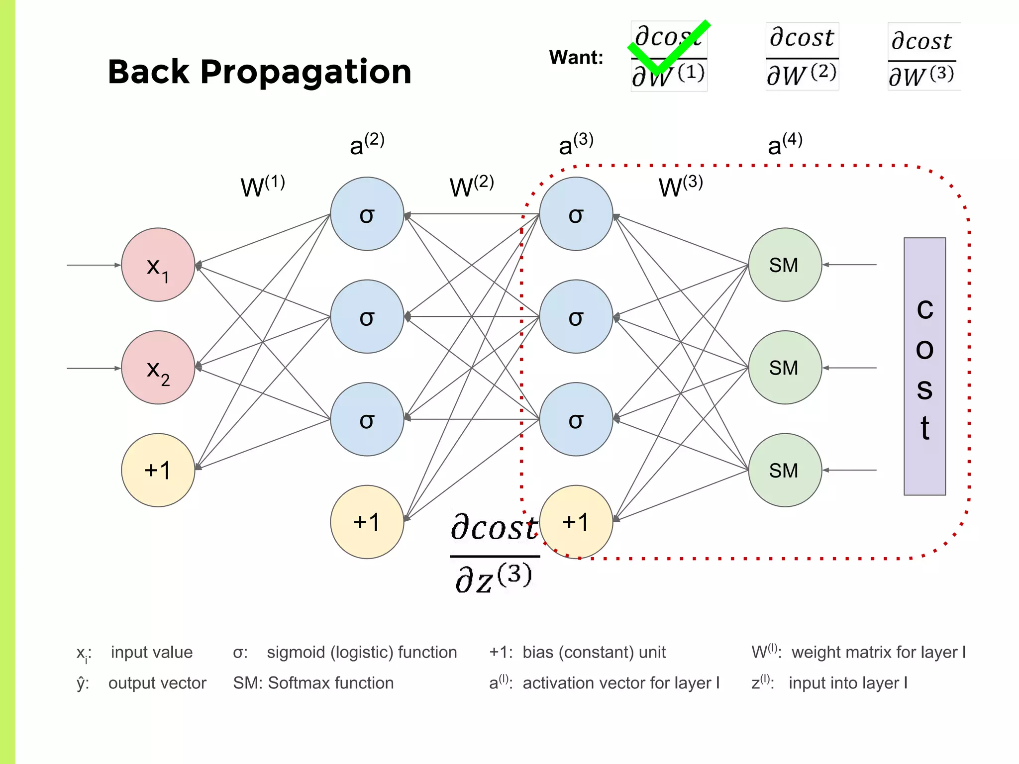
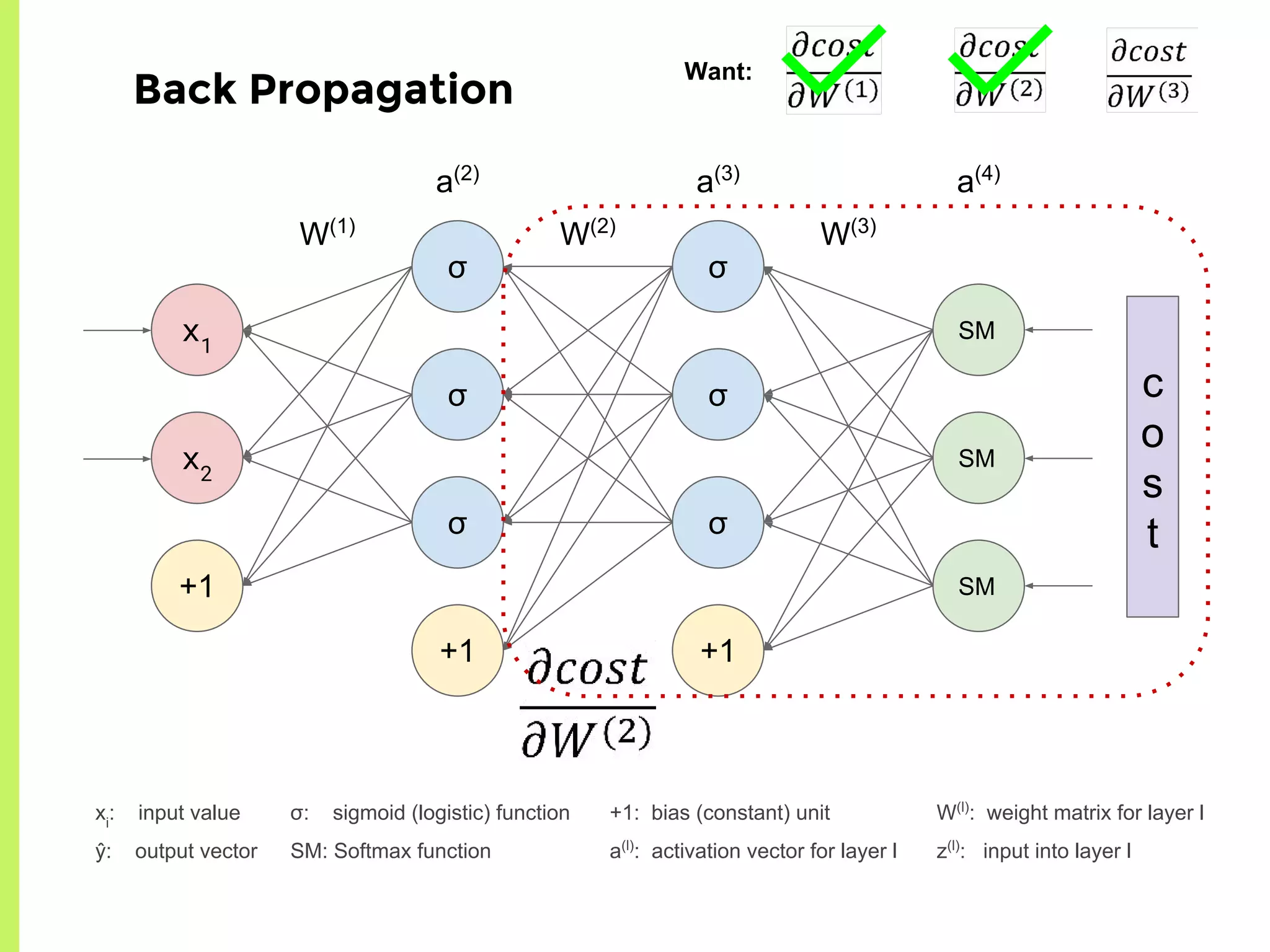
Concept of Neural Networks: chaining non-linear functions, adjustable parameters (weights), and architecture representation.
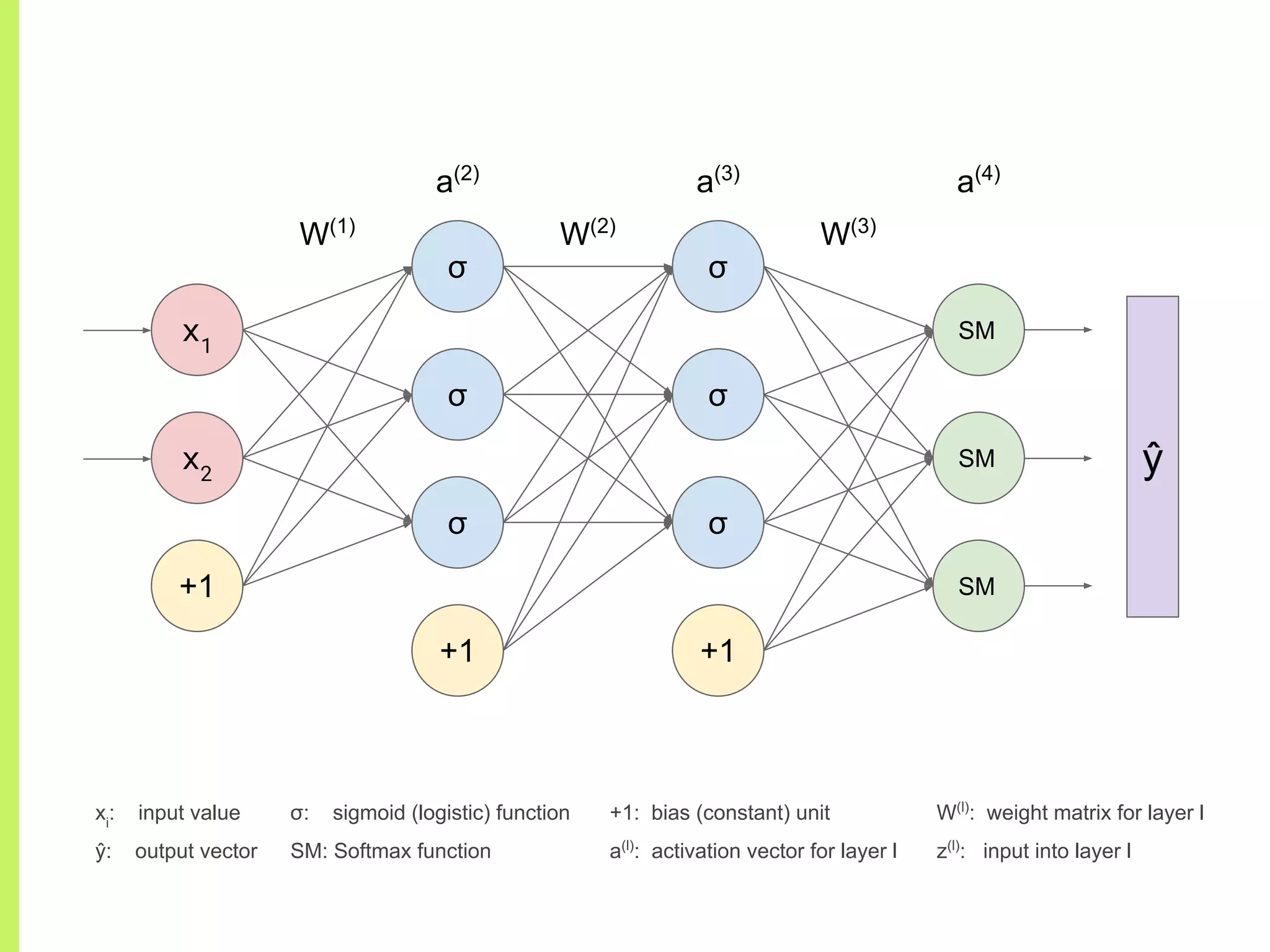
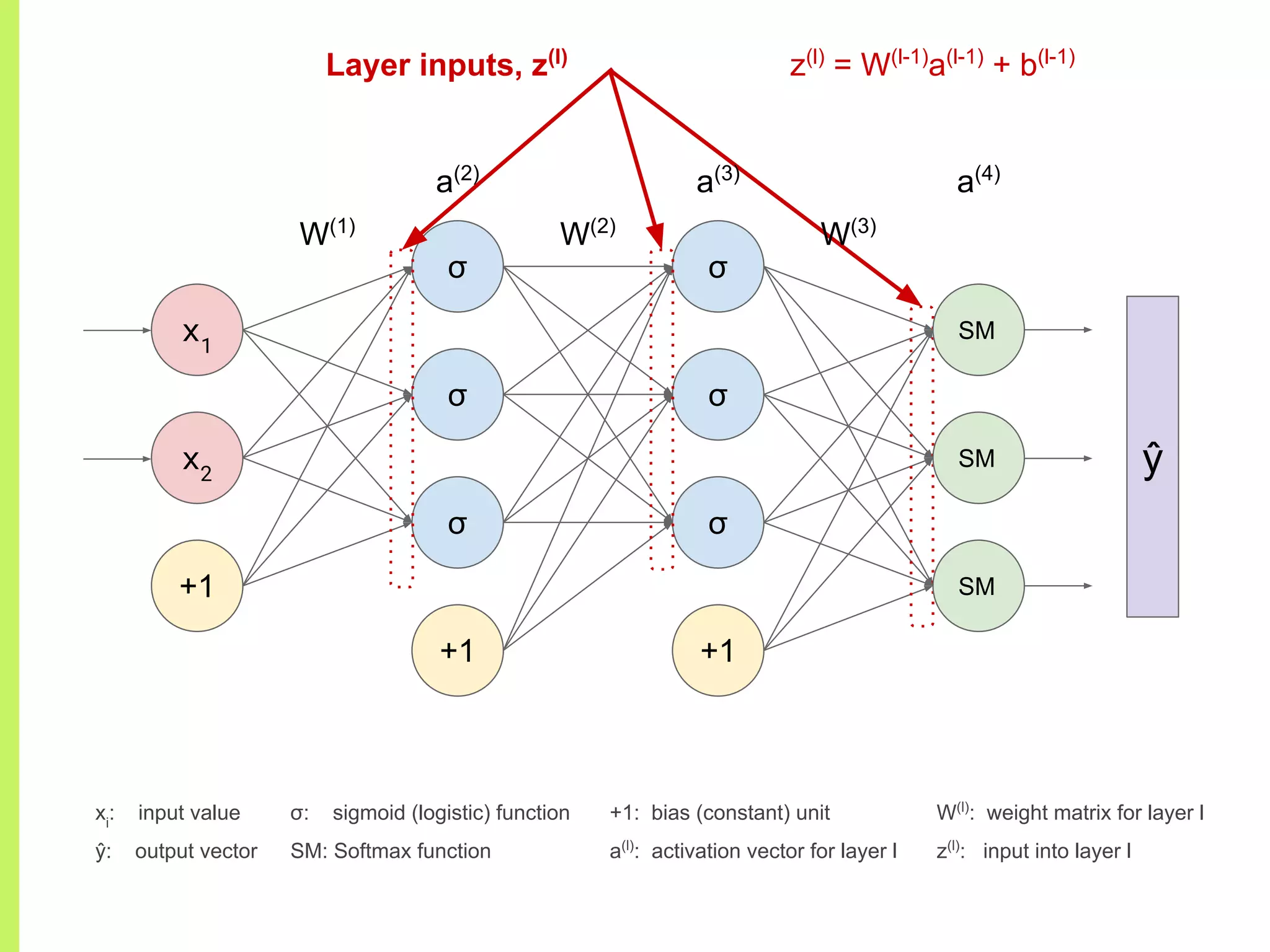
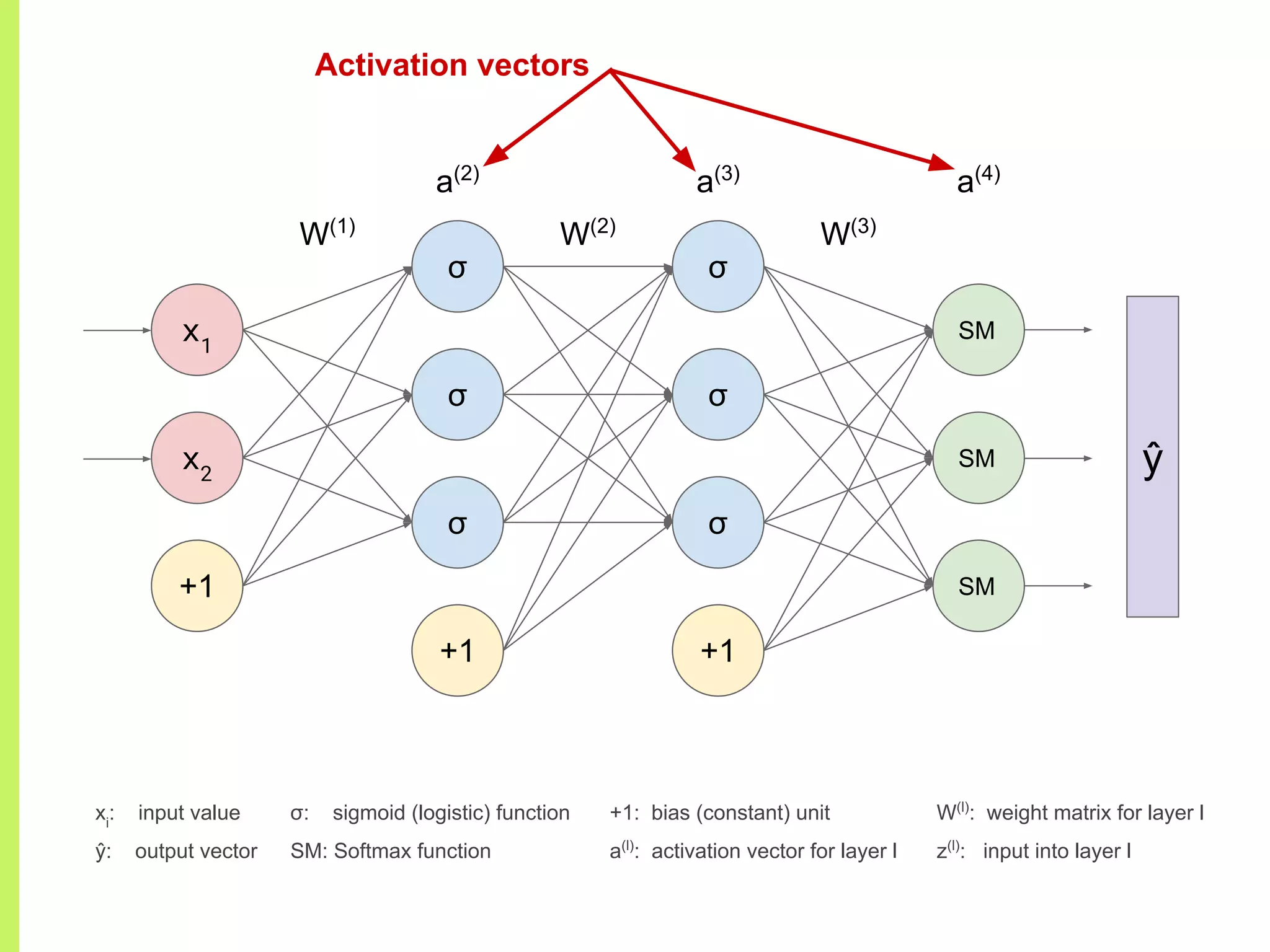
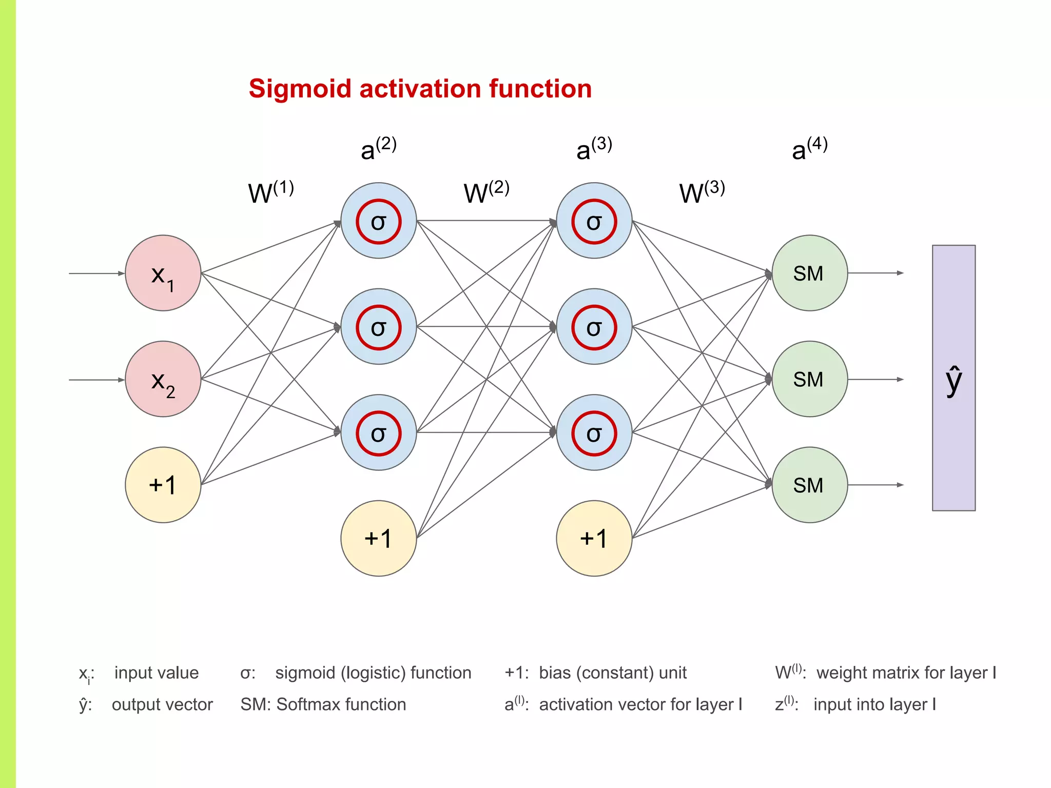
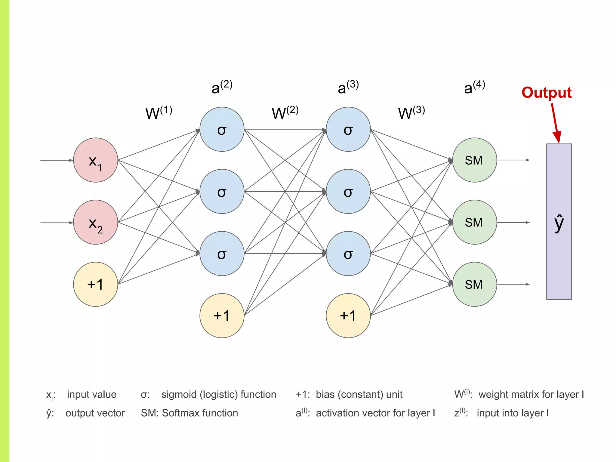
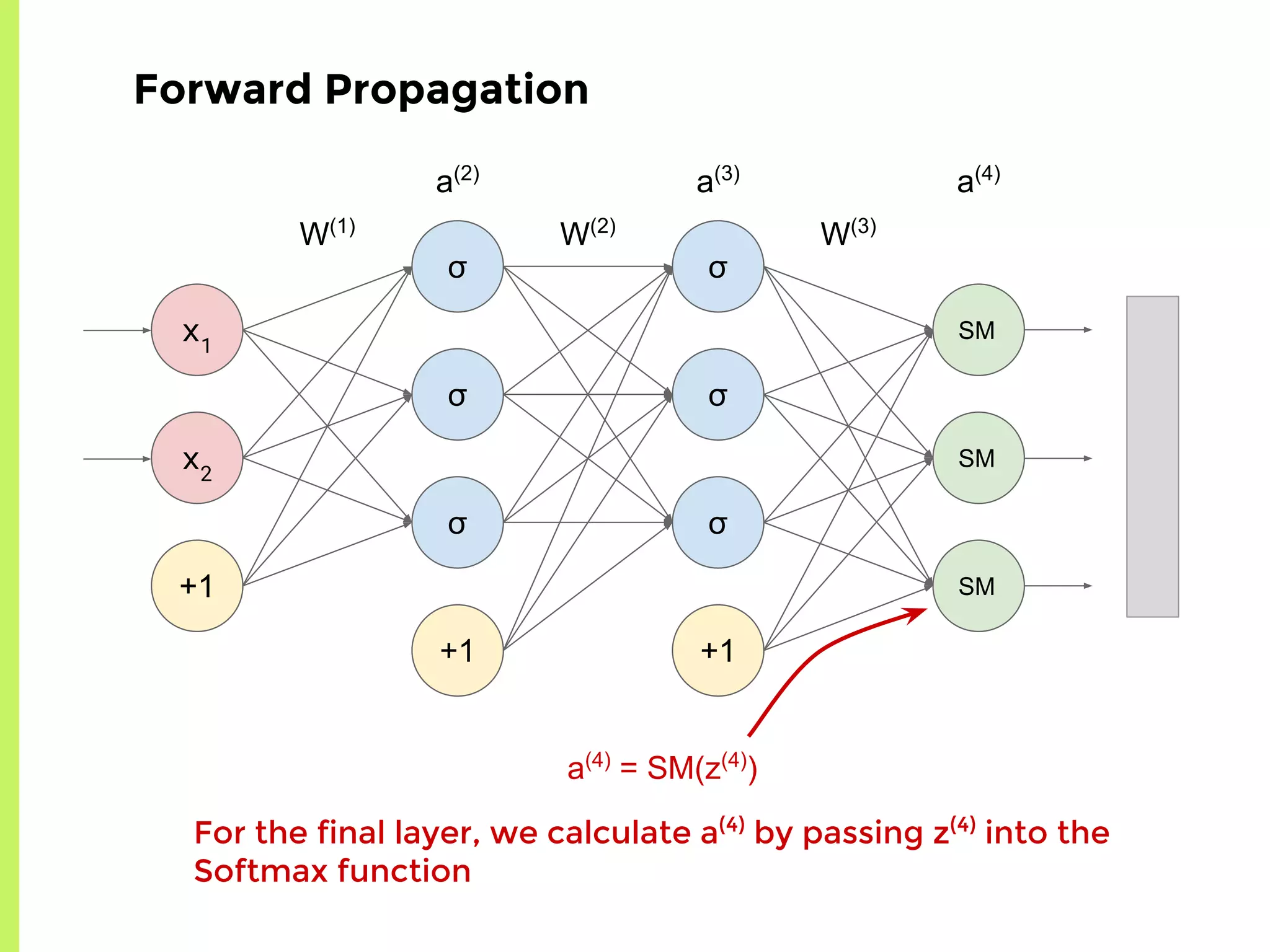
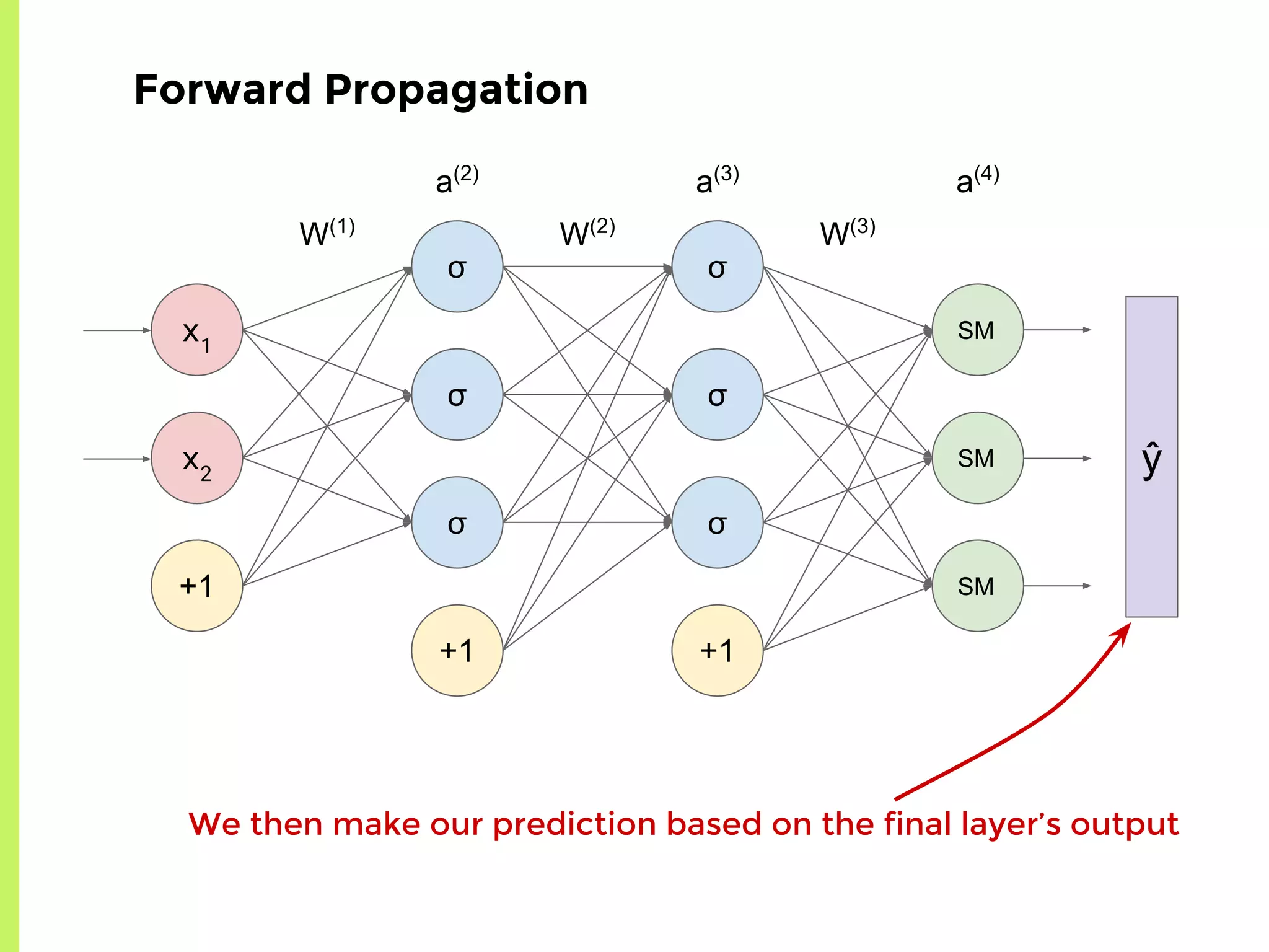
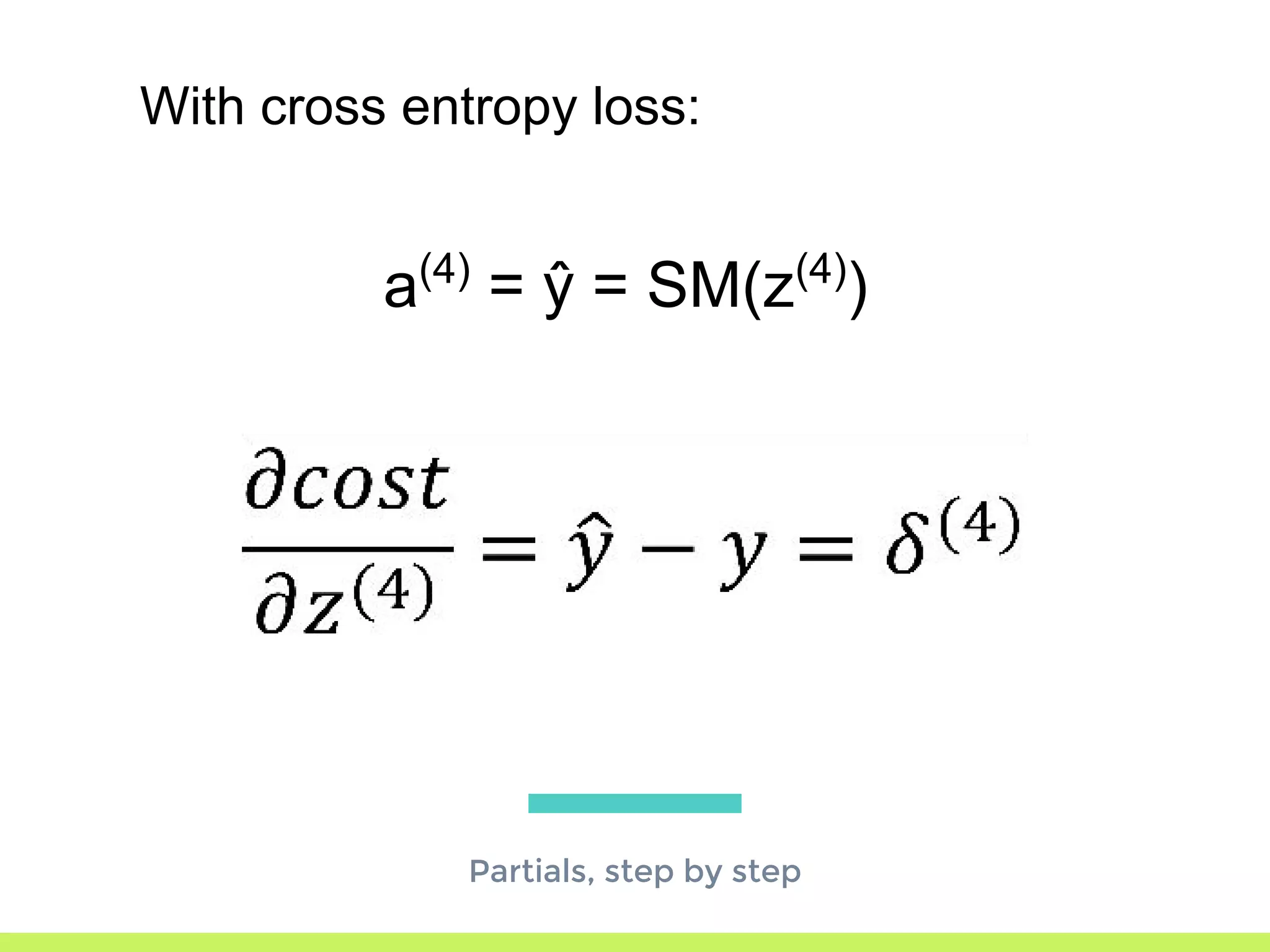
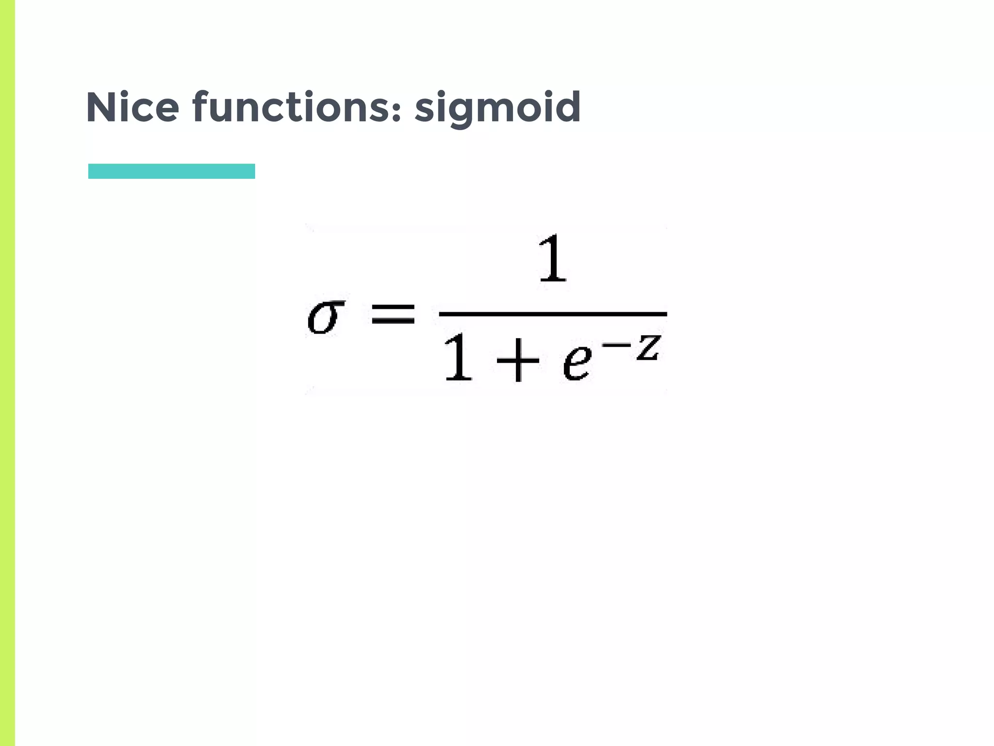
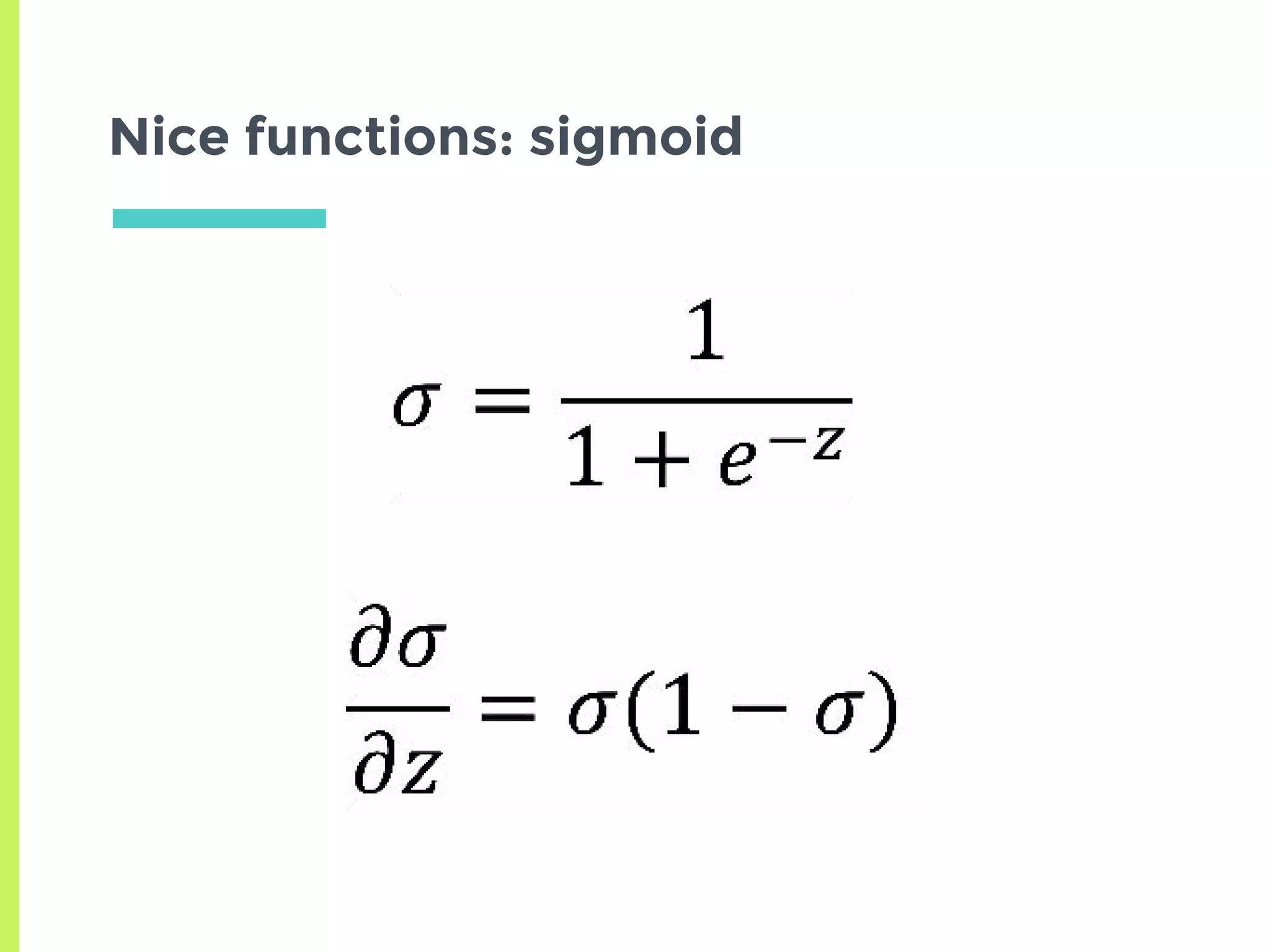
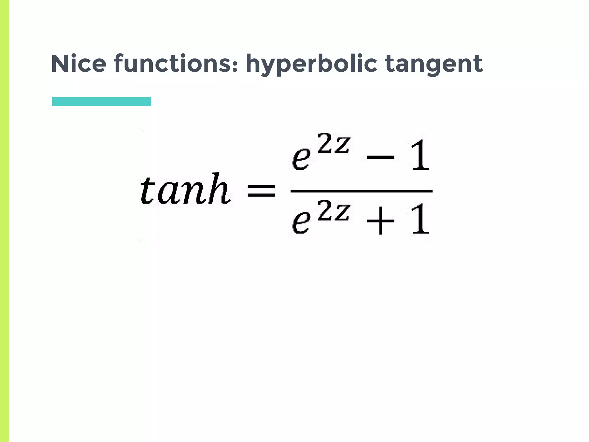
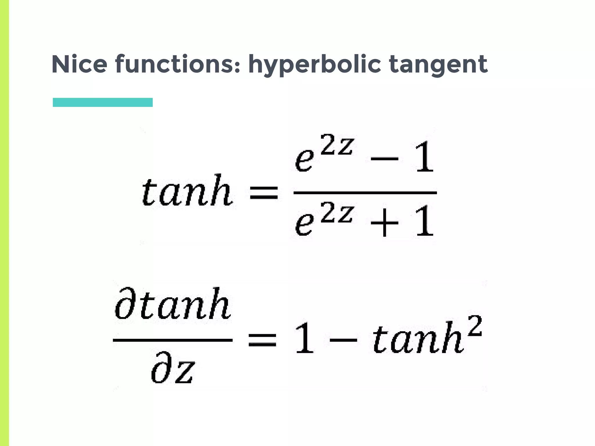
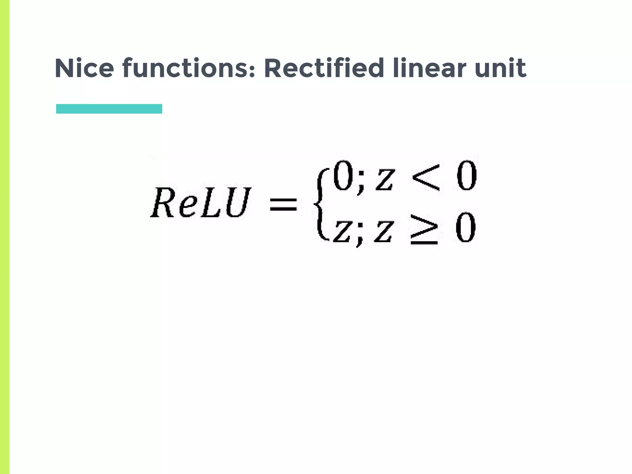
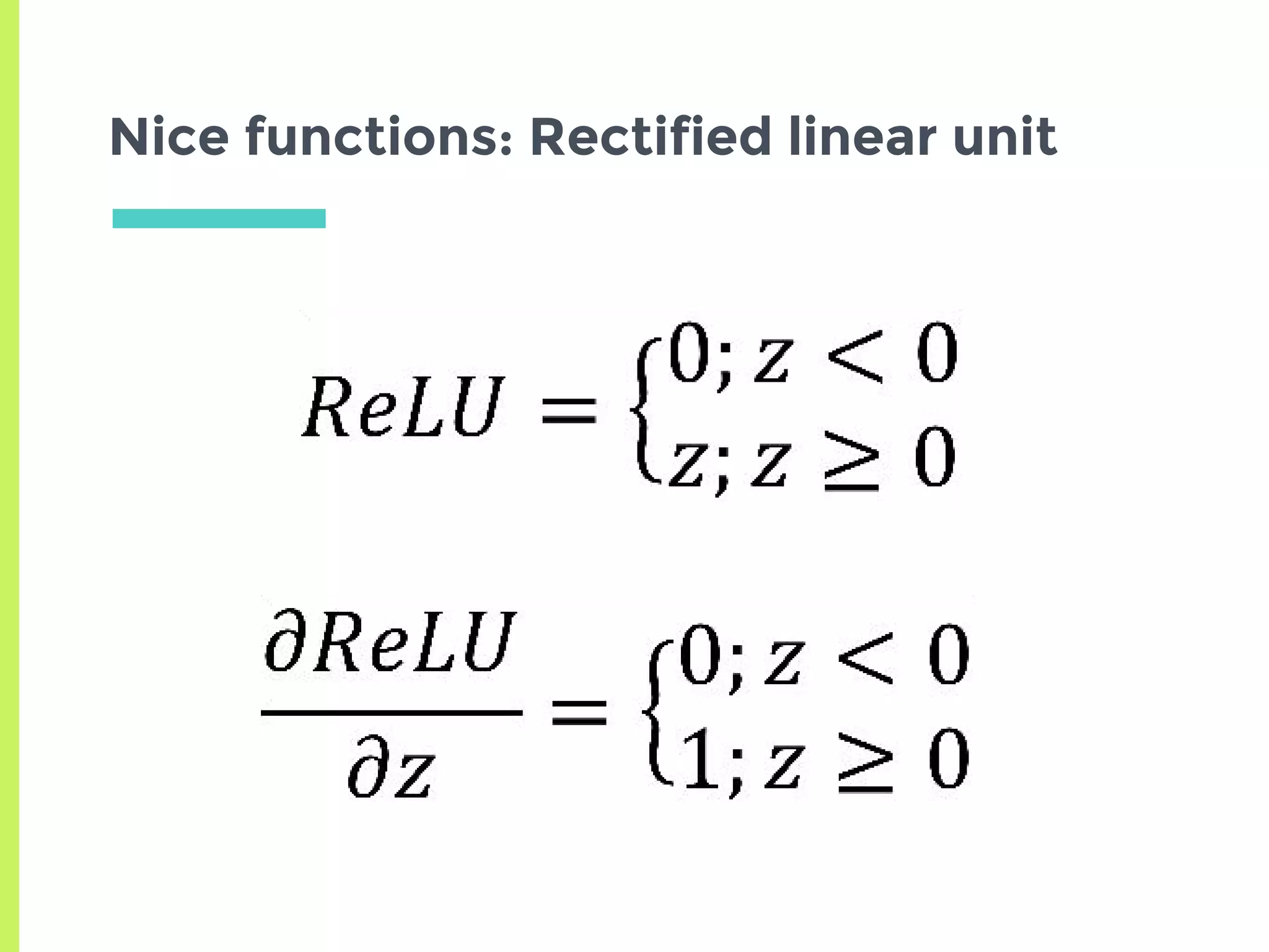
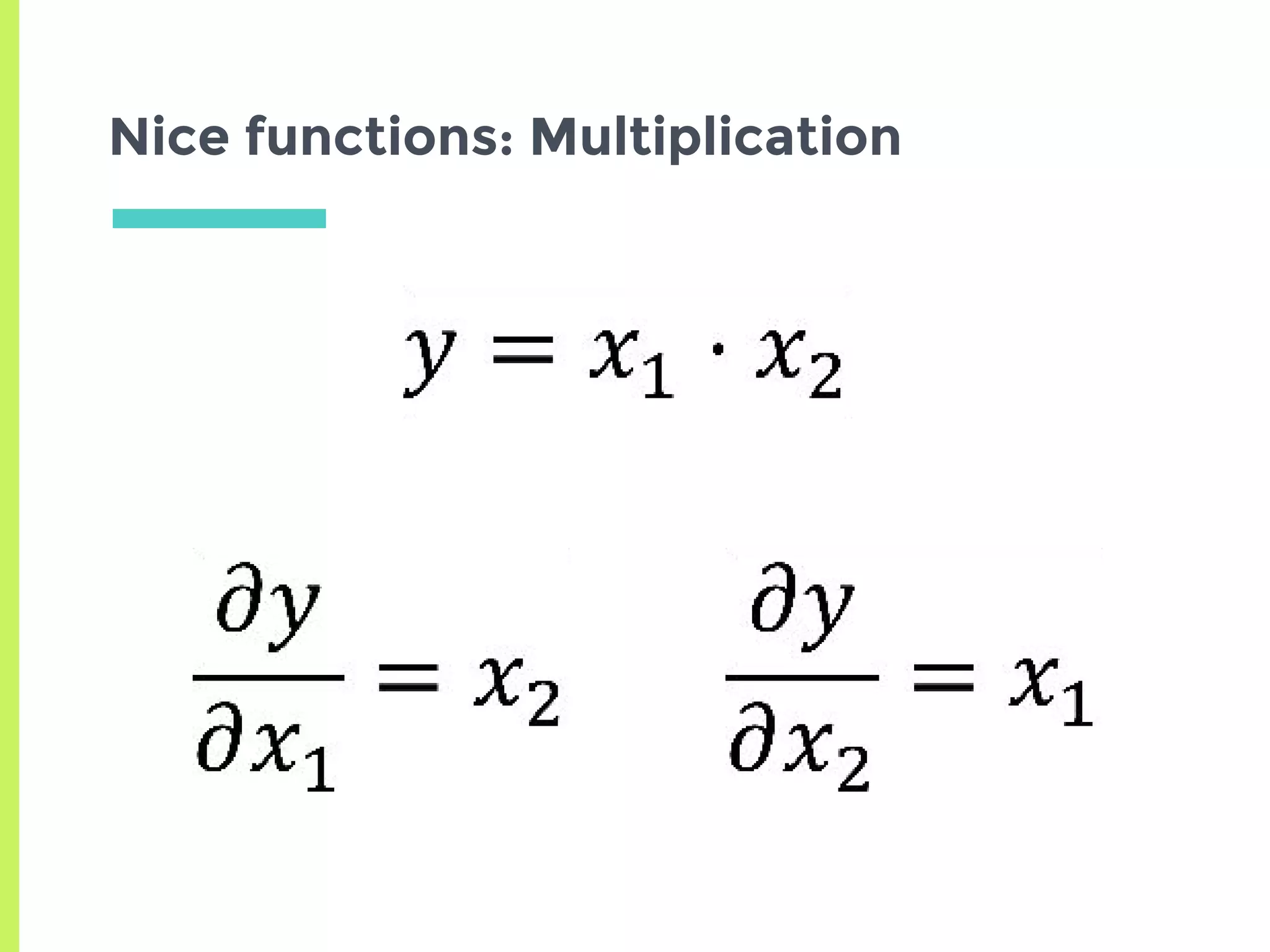
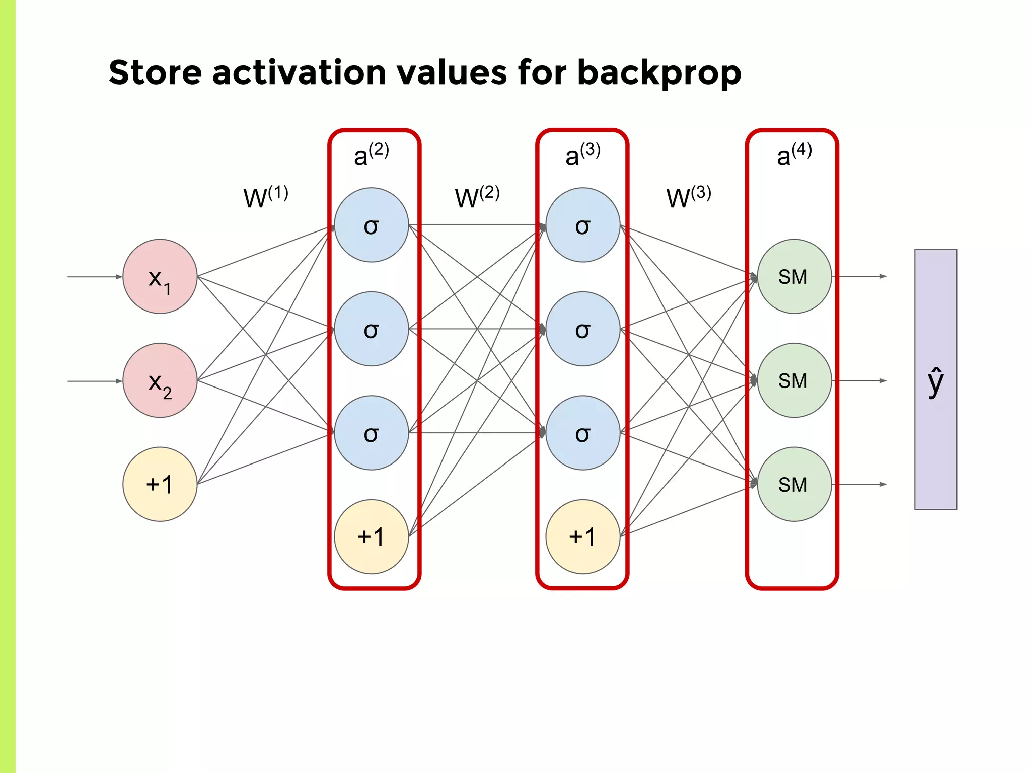
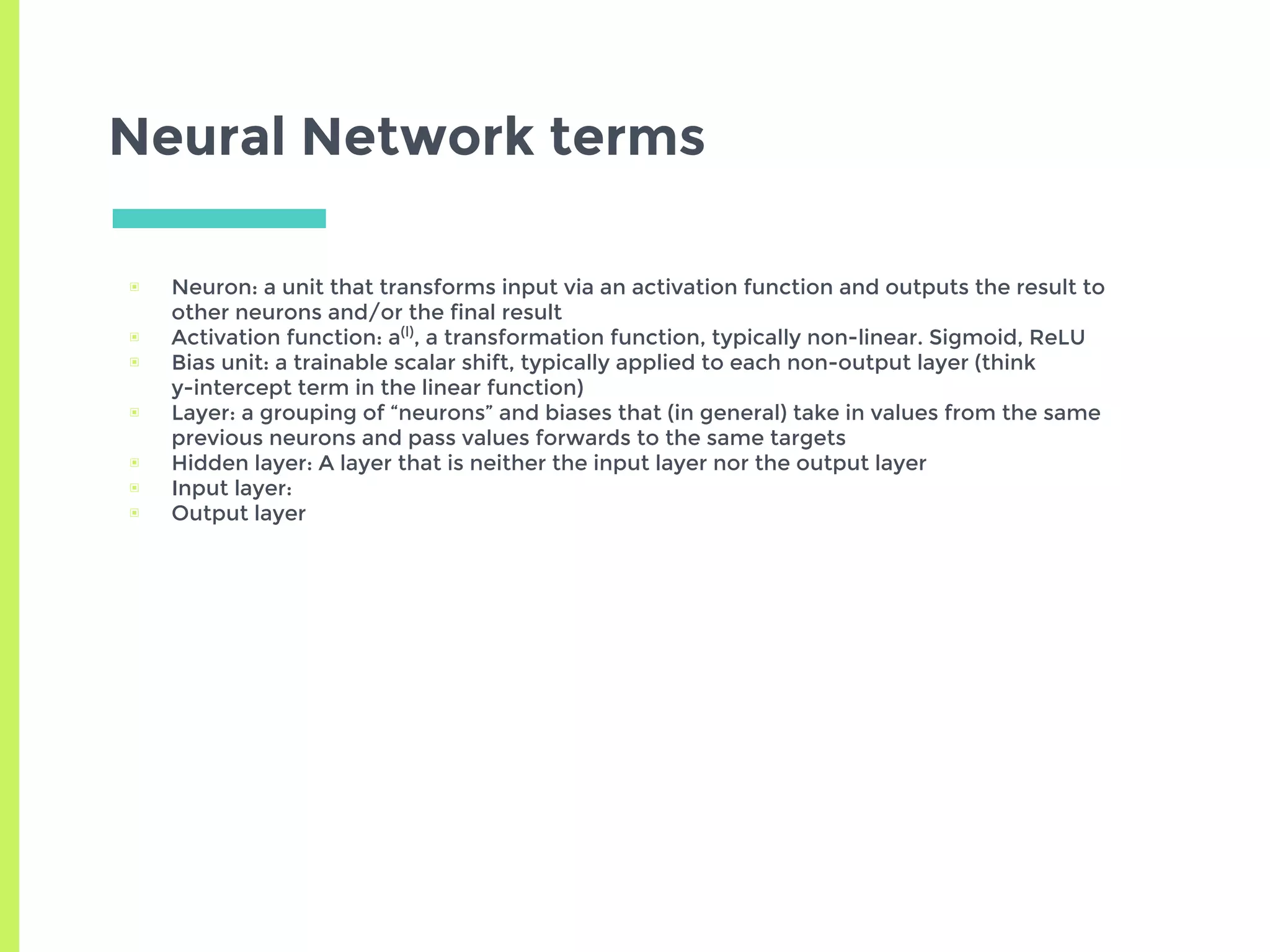
Details on various neural network layers including activation functions such as sigmoid and softmax, and their roles in computation.
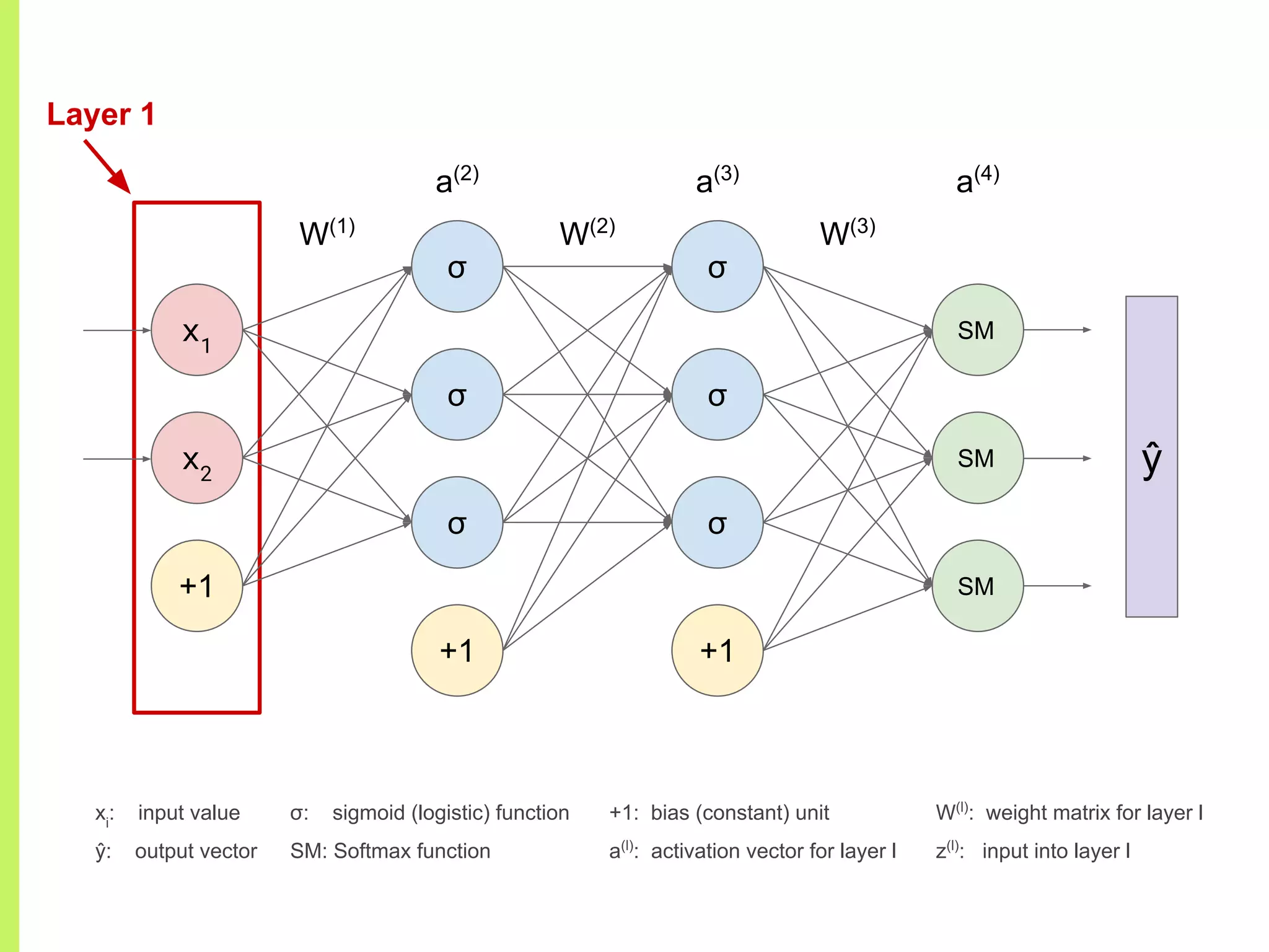
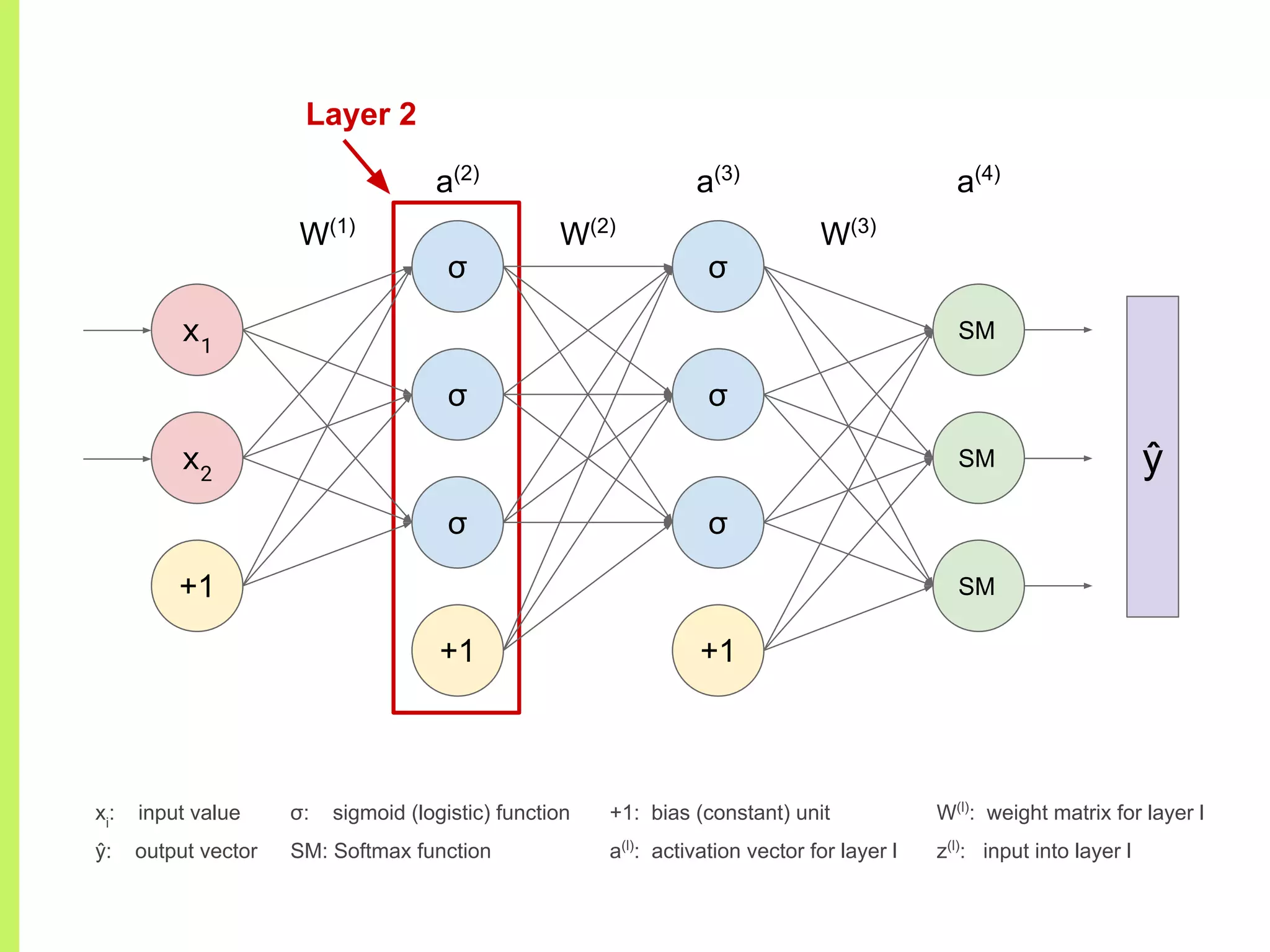
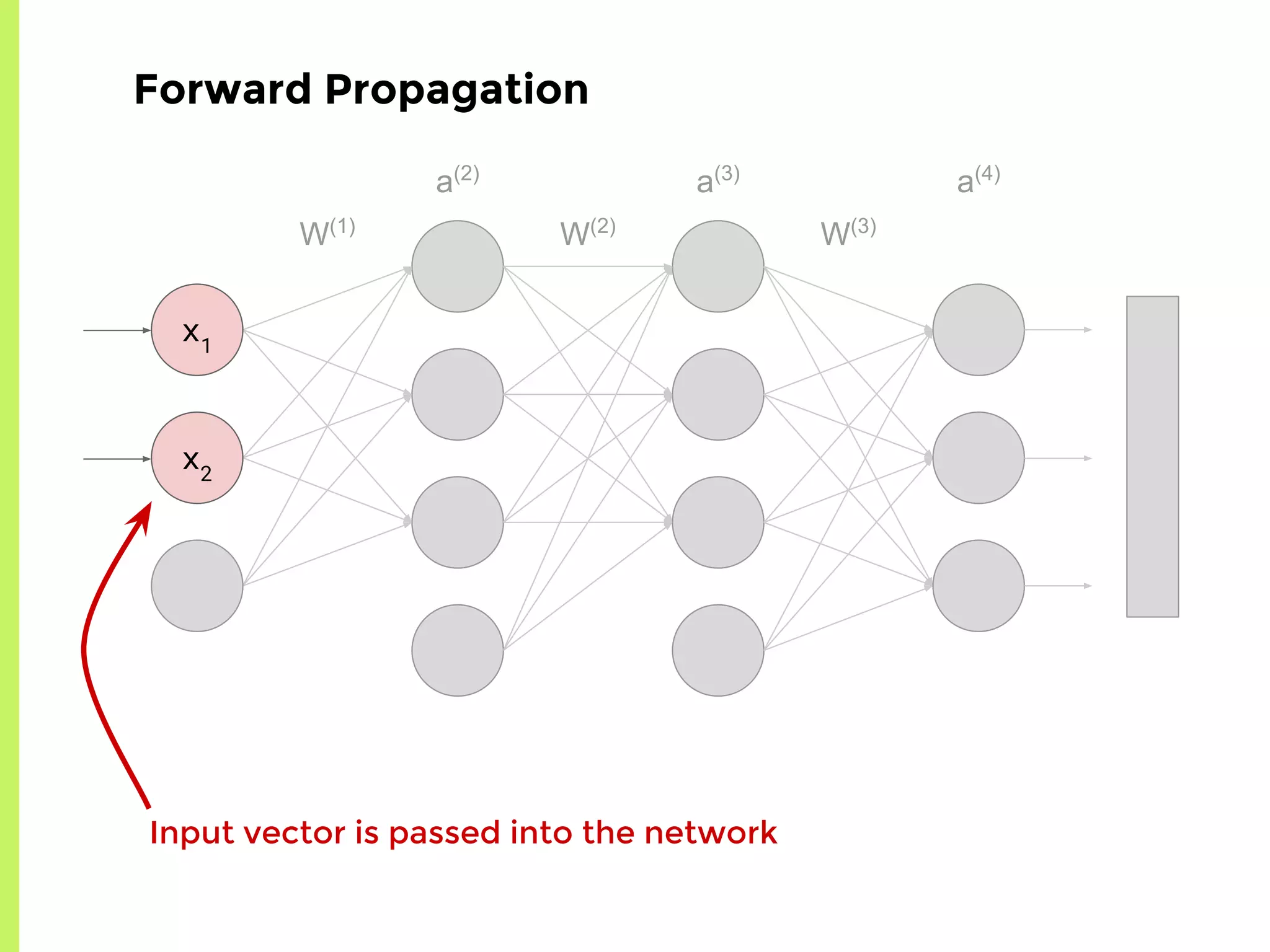
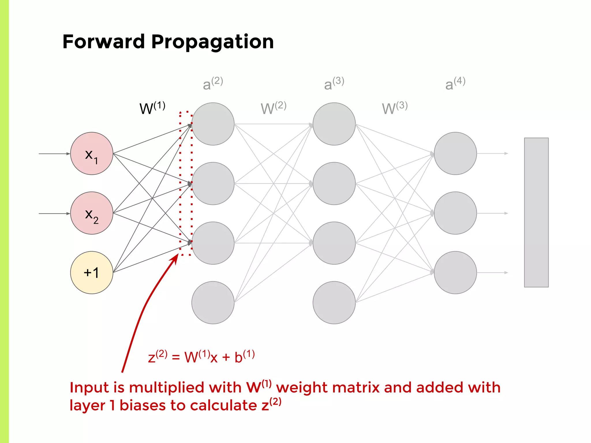
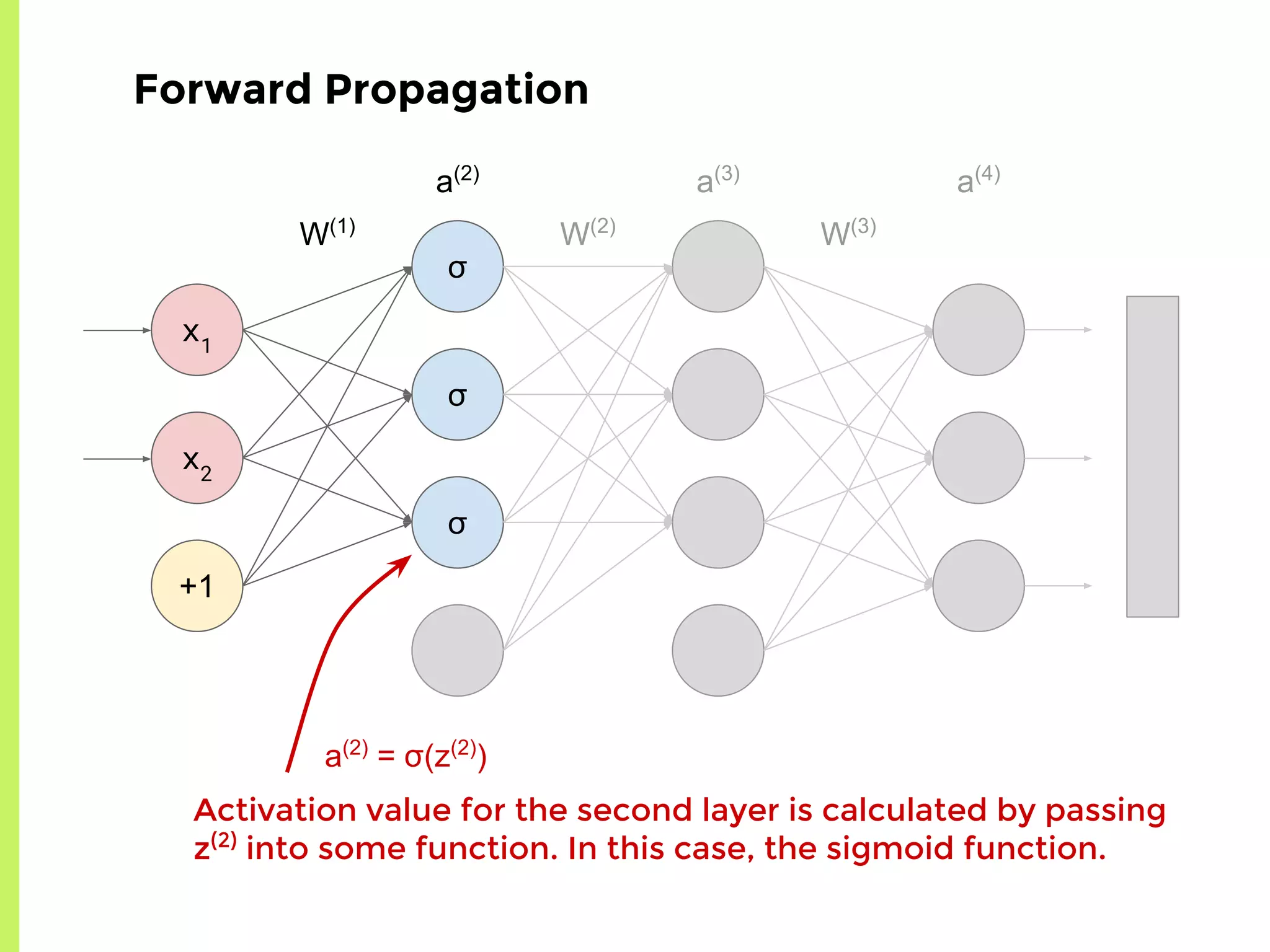
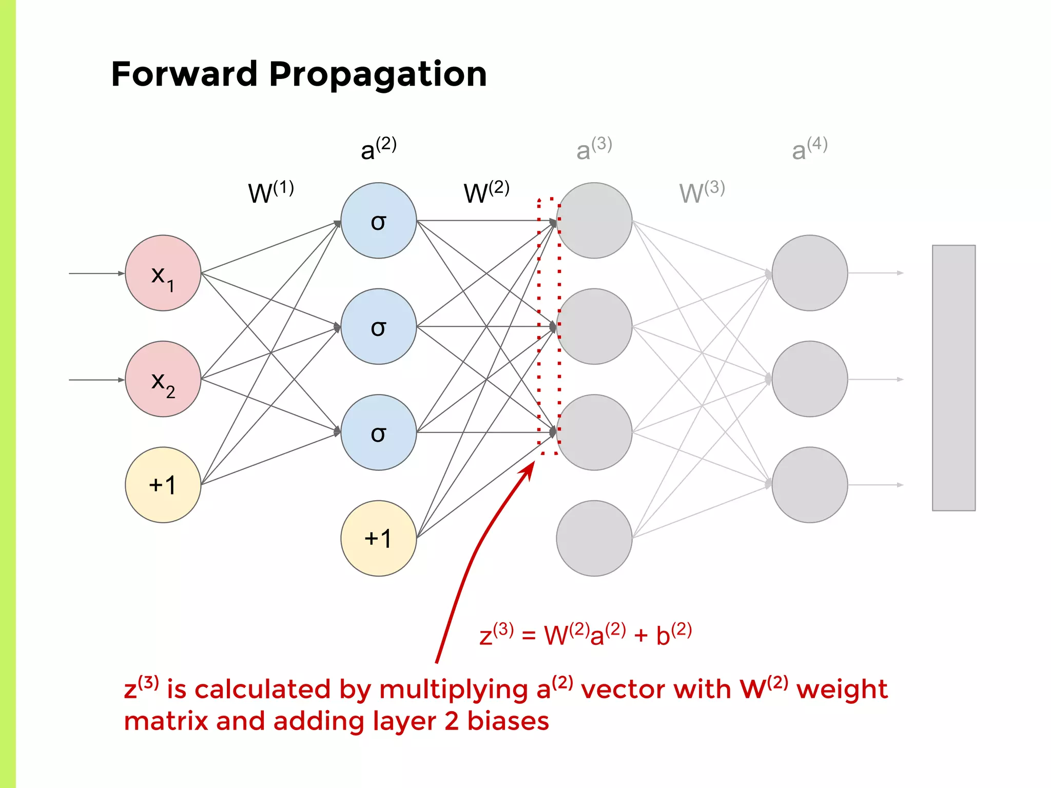
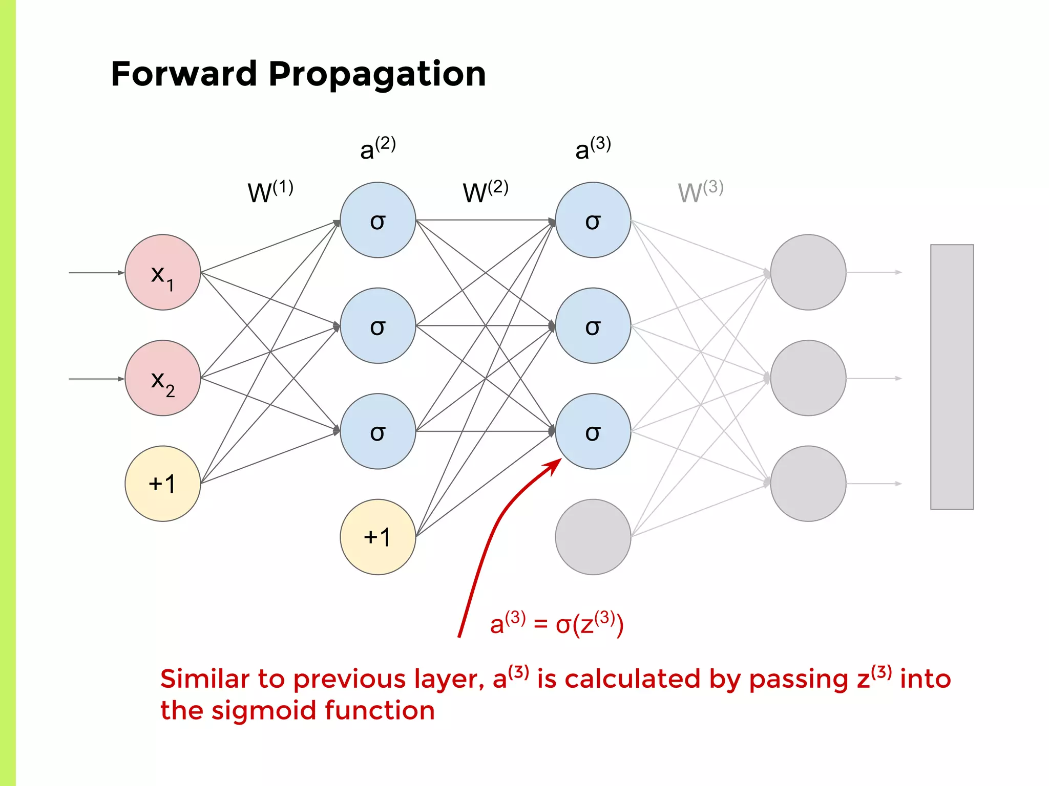
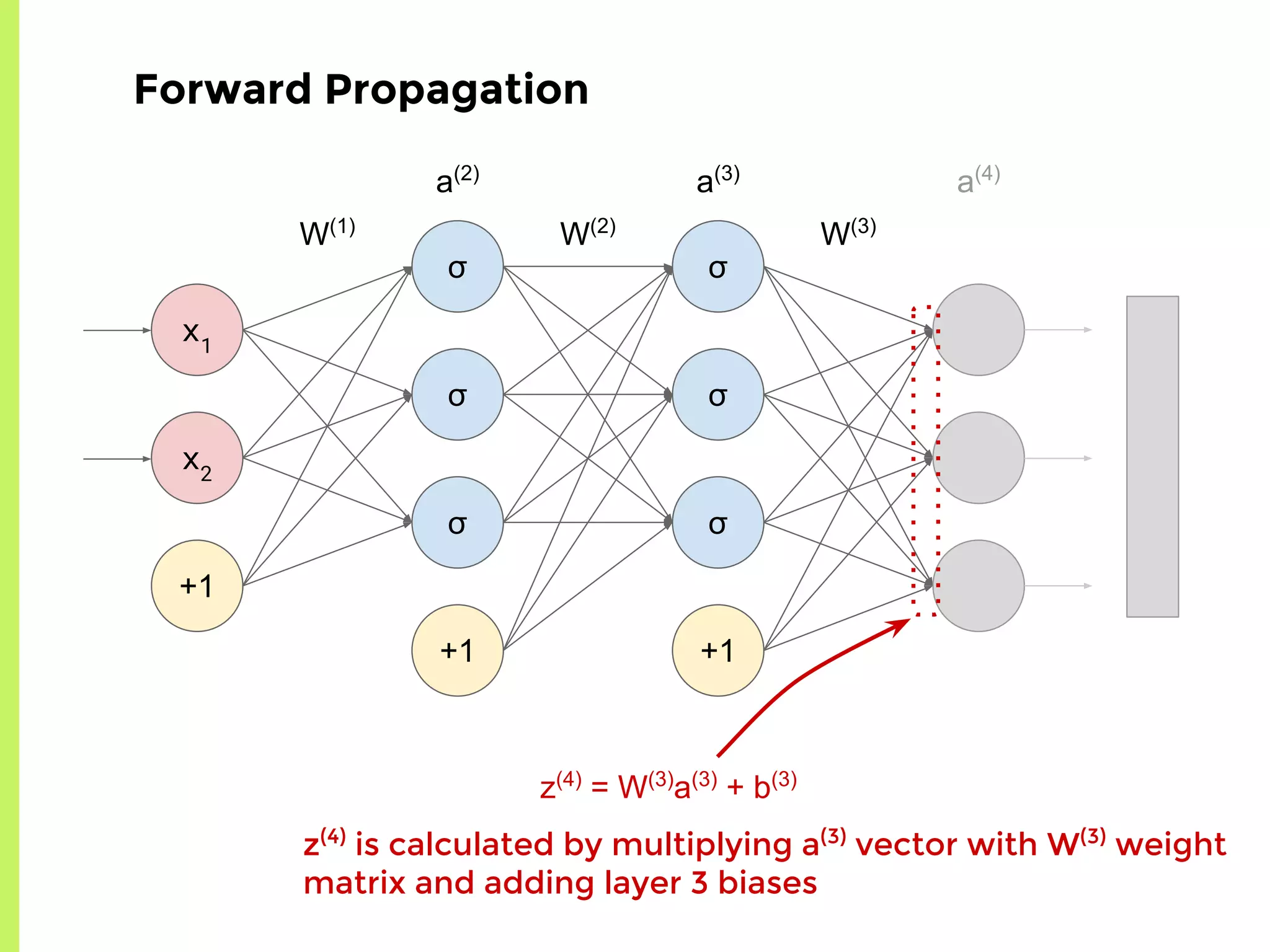
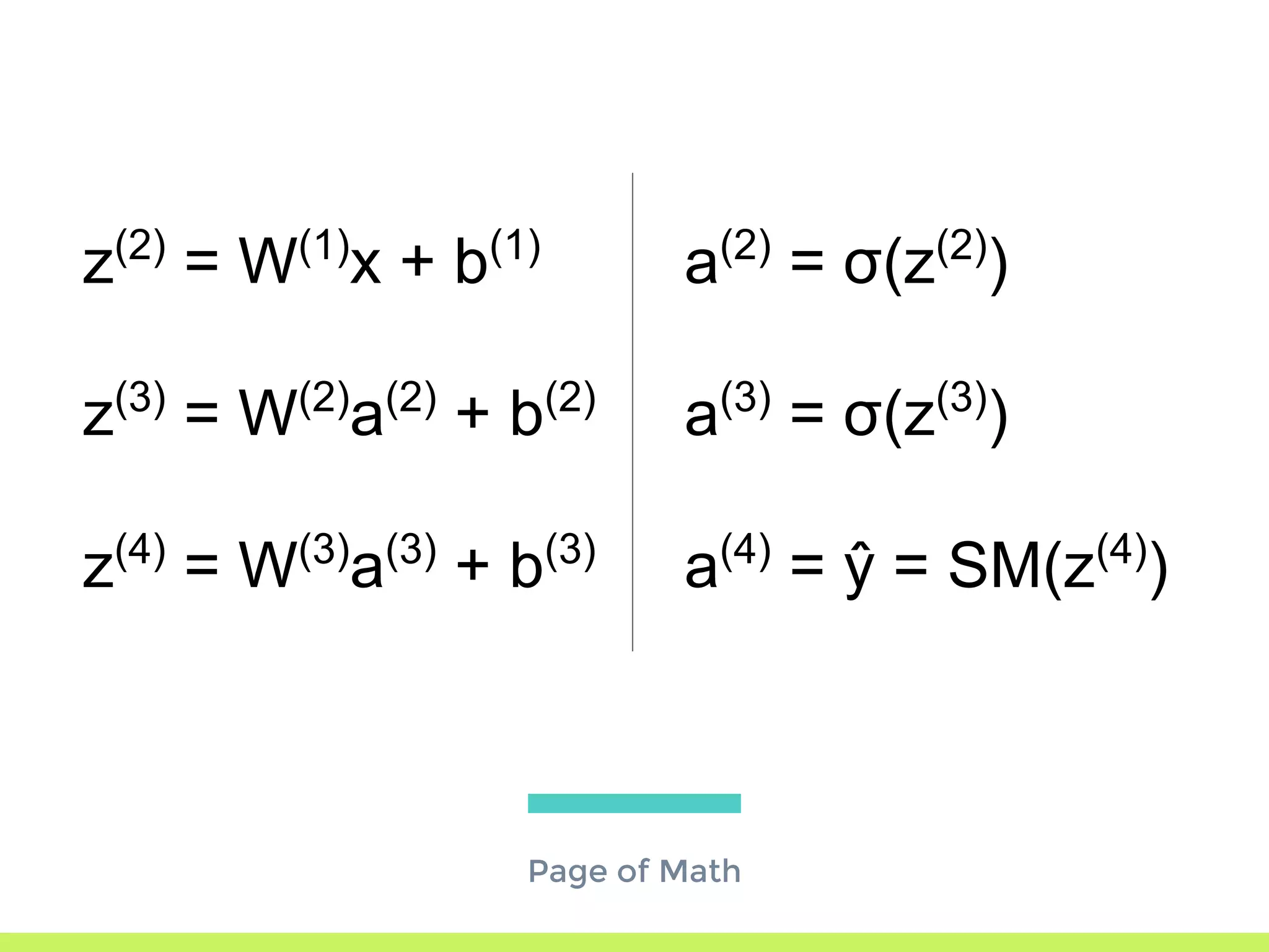
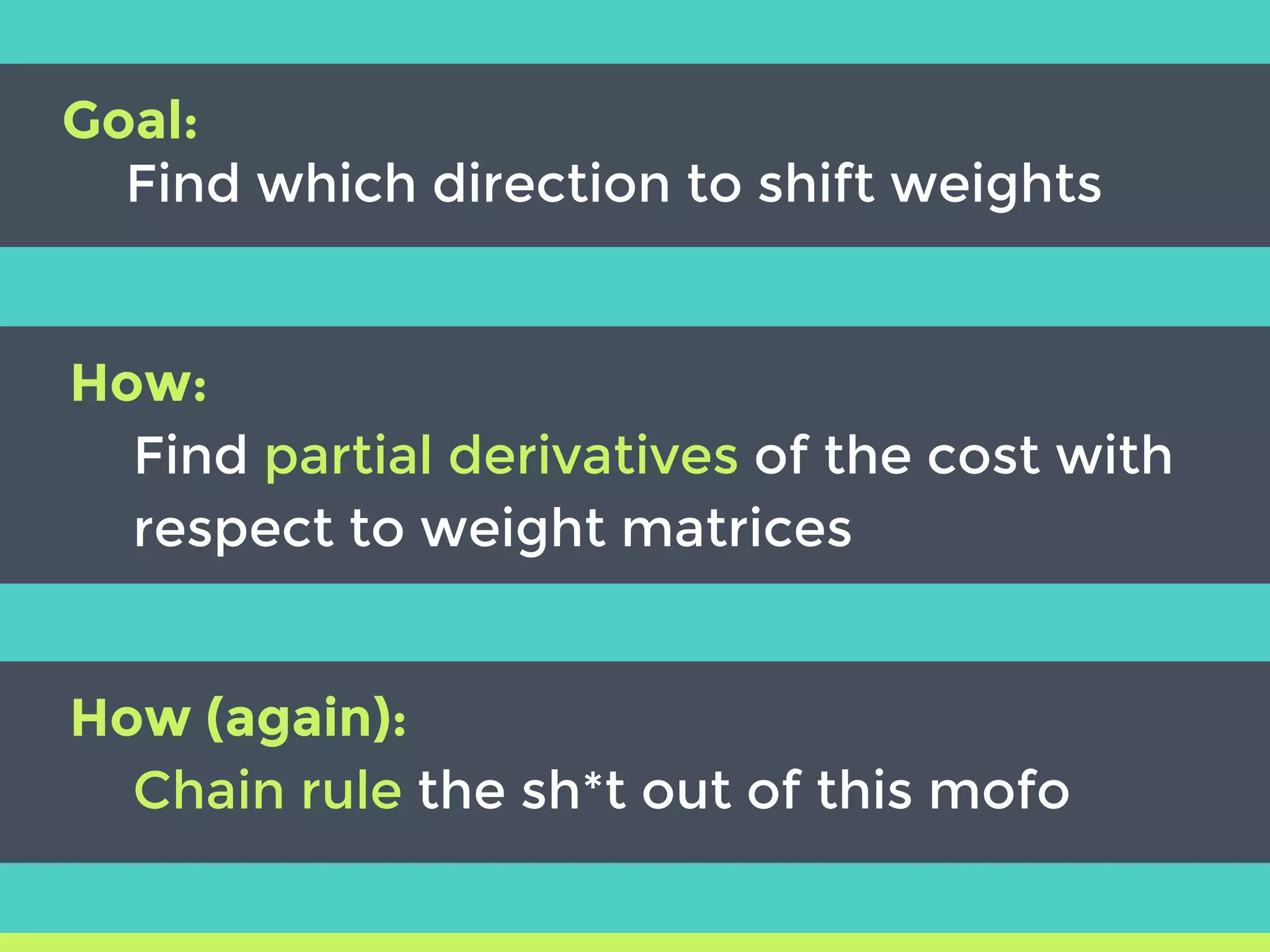
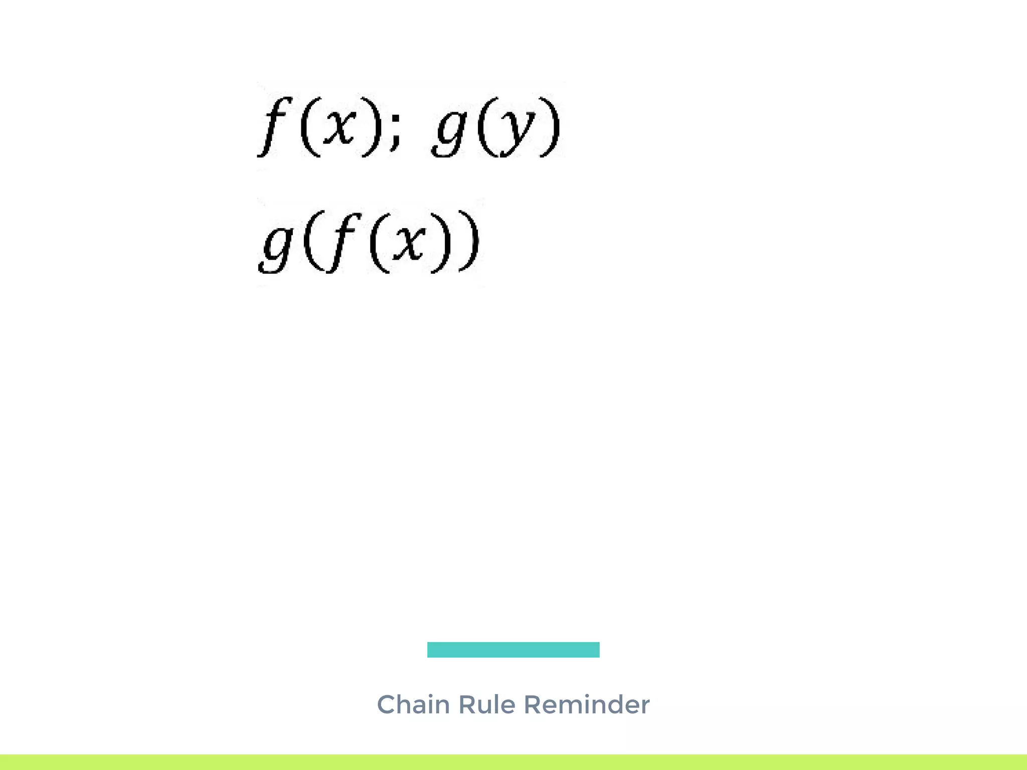
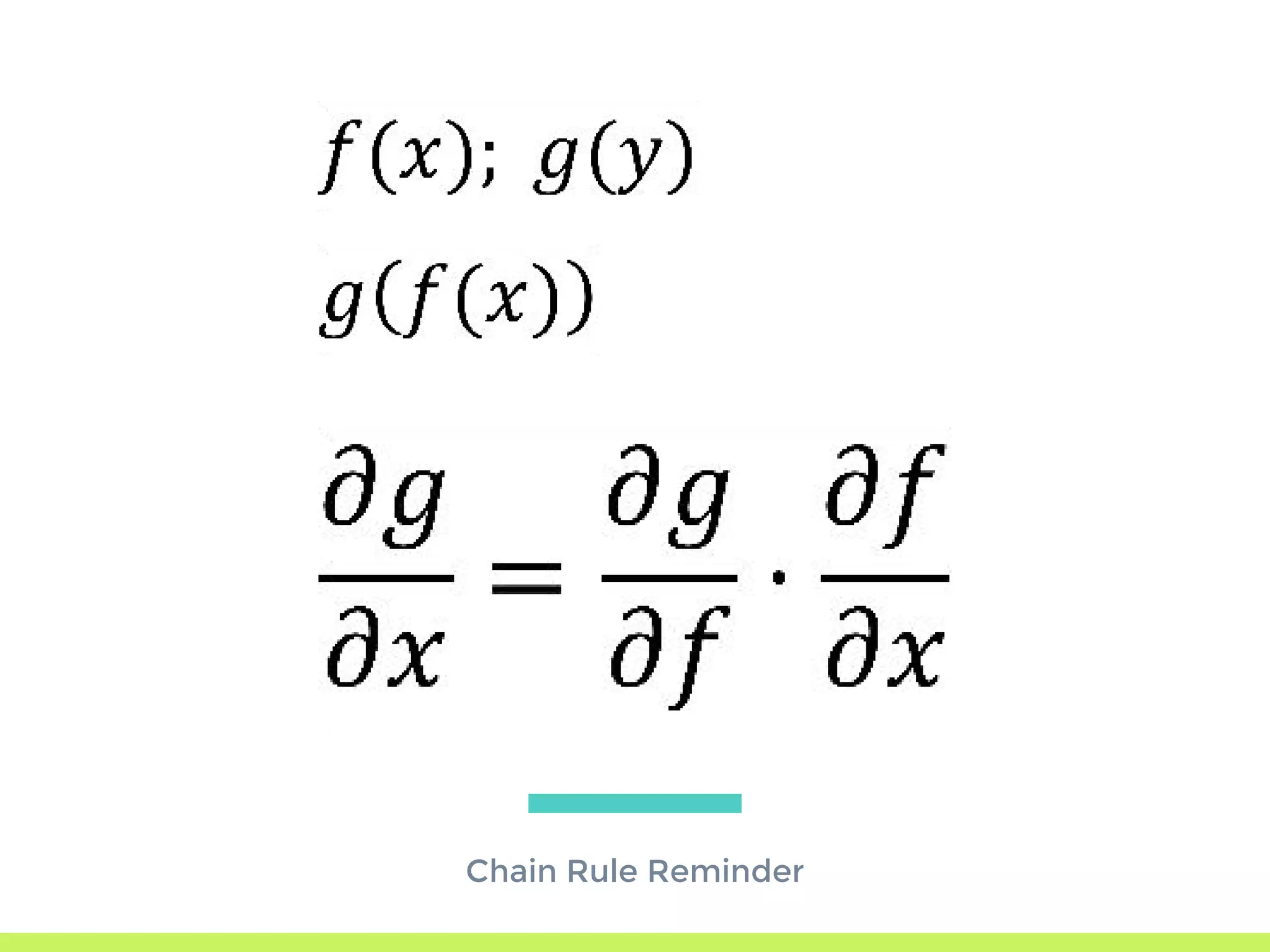
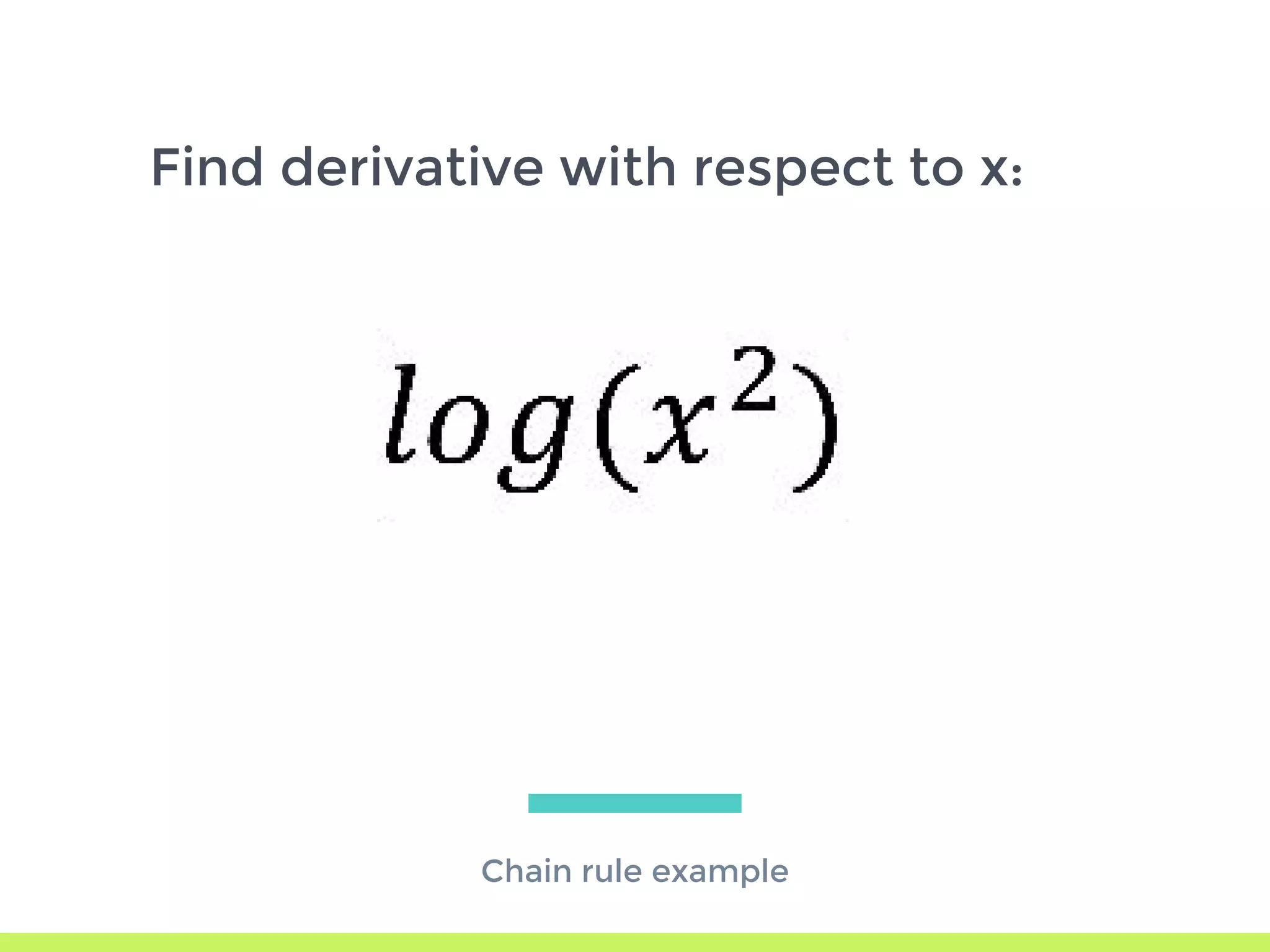
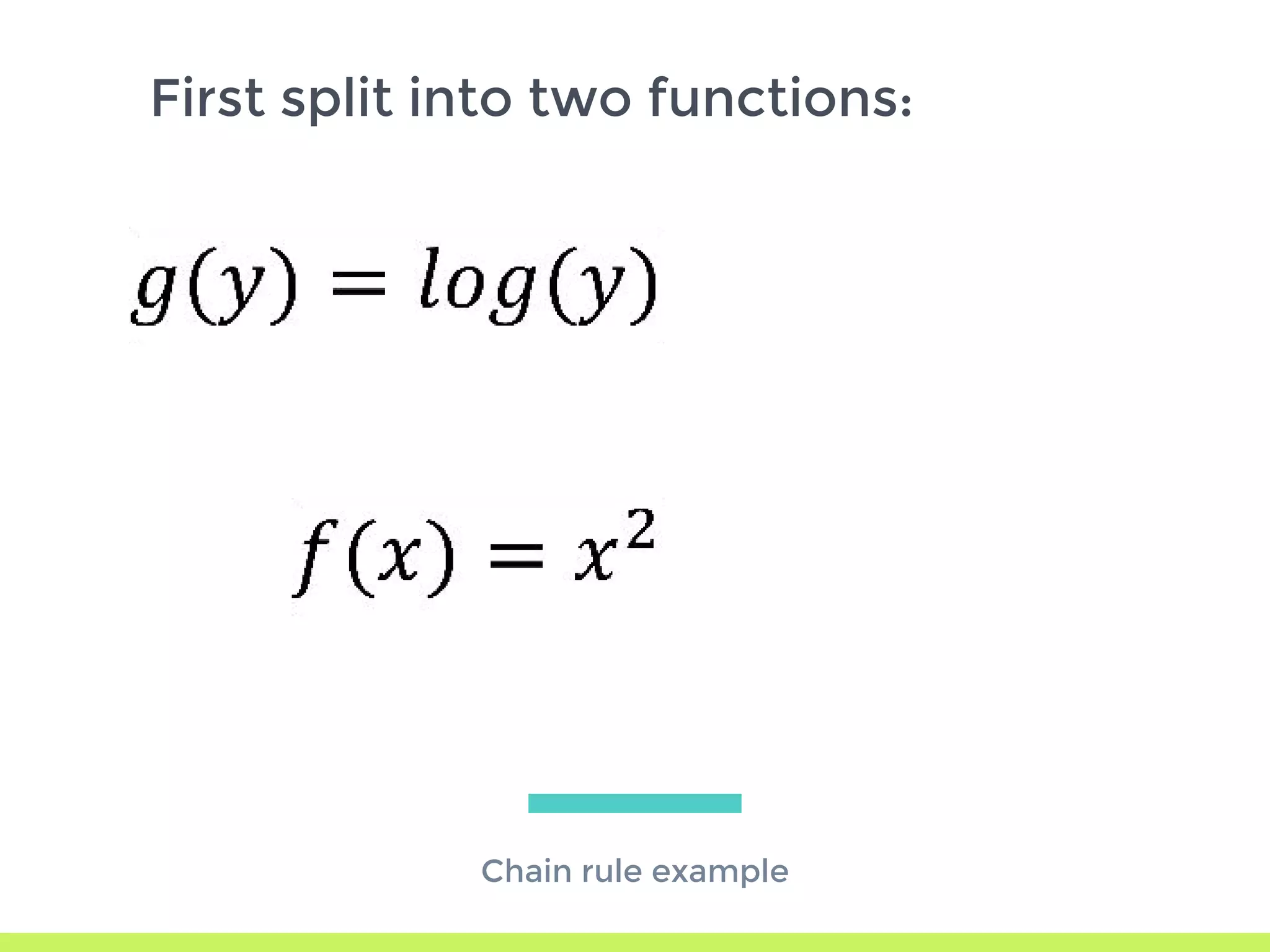
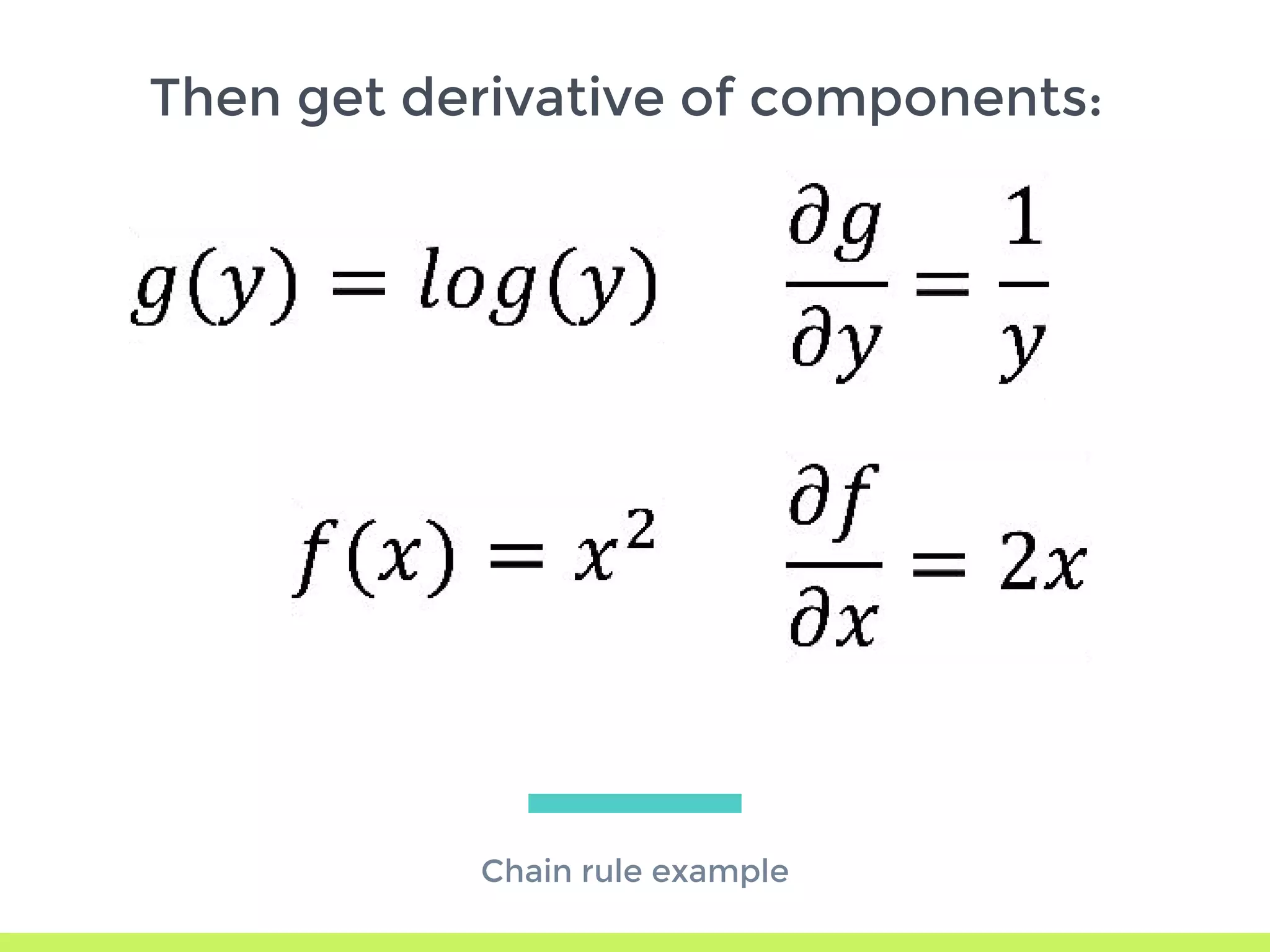
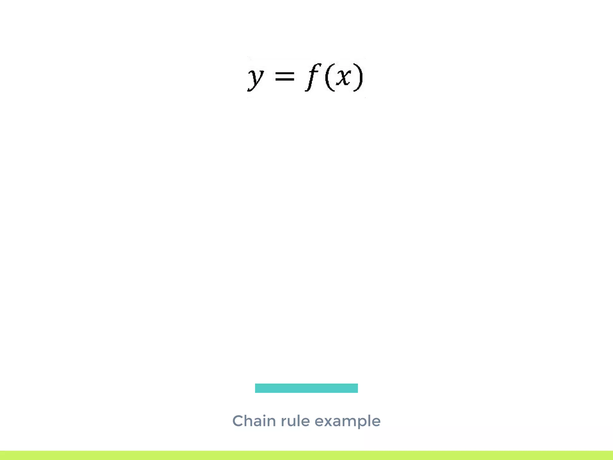
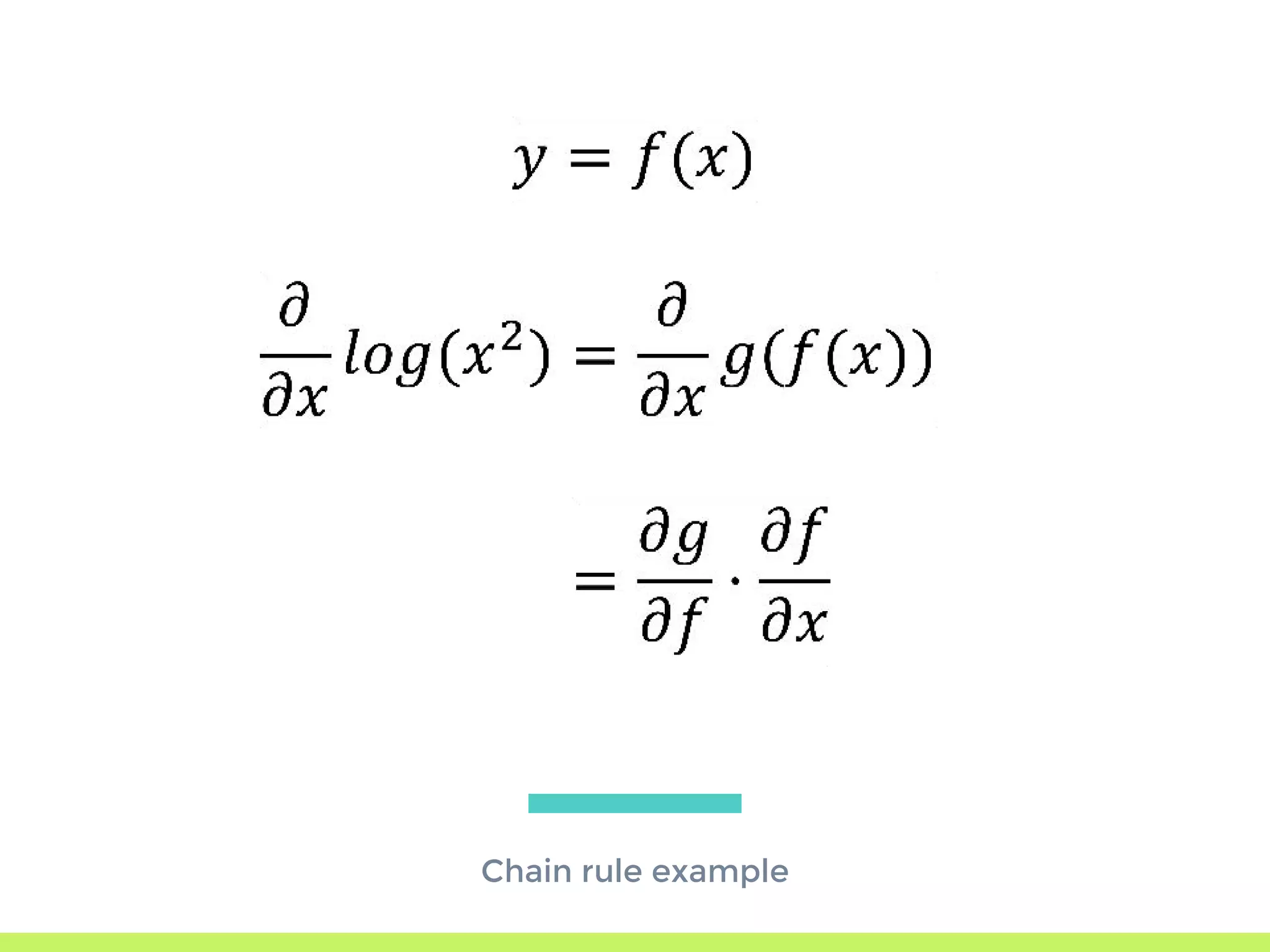
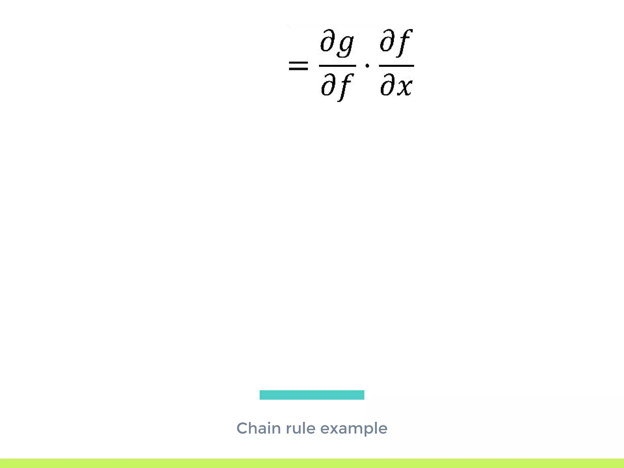
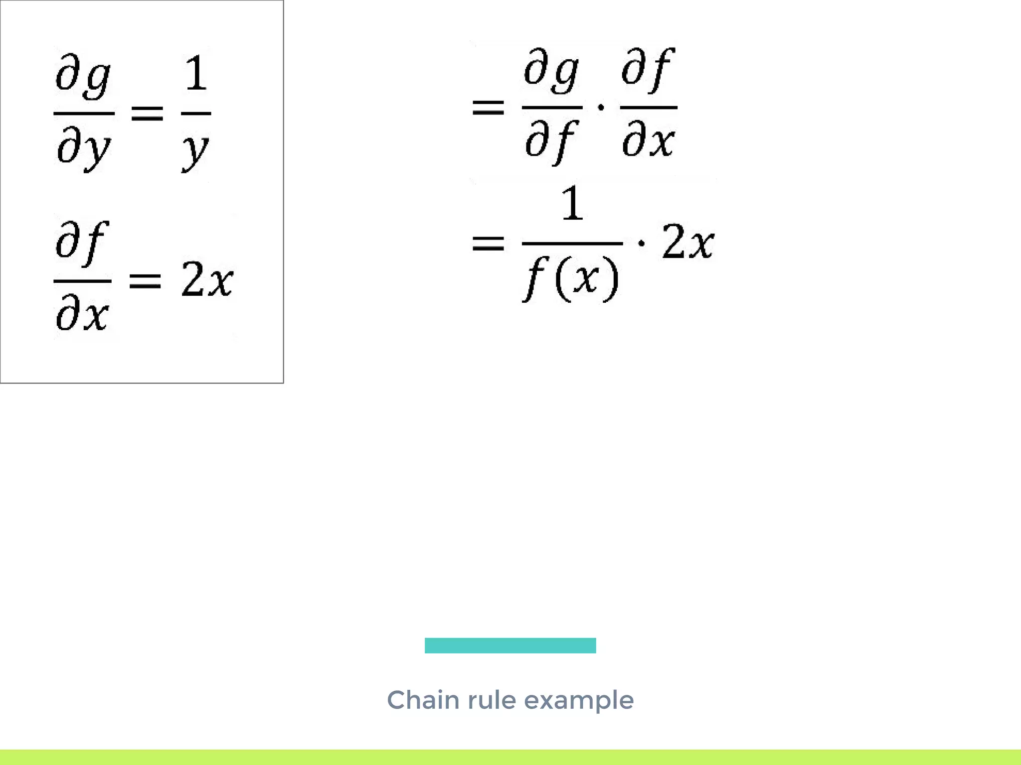
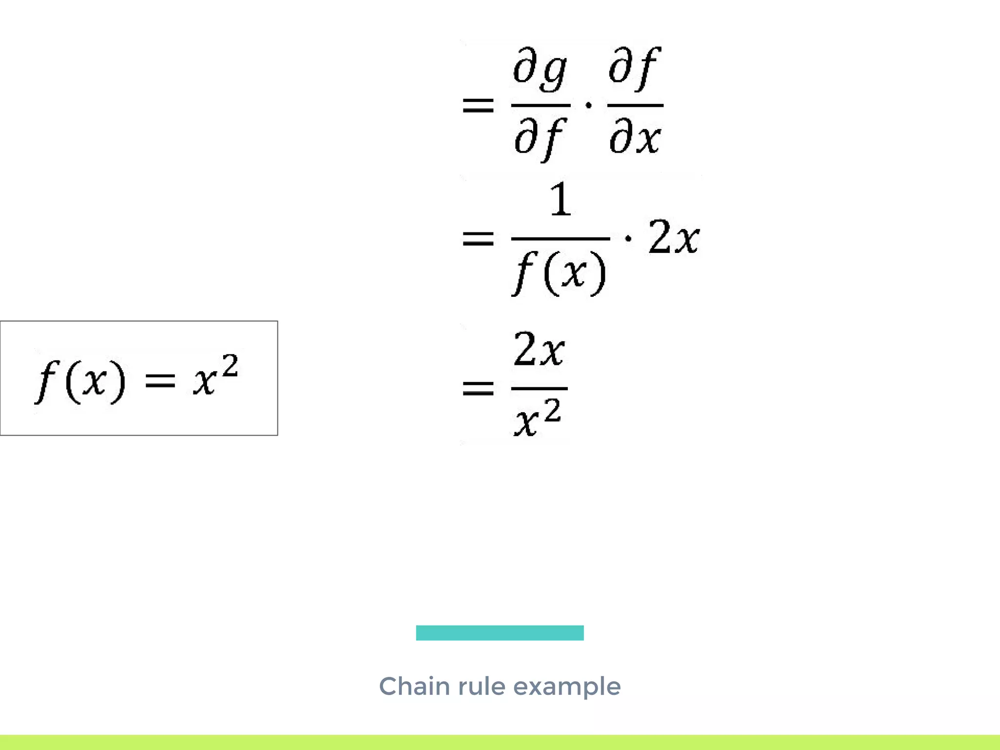
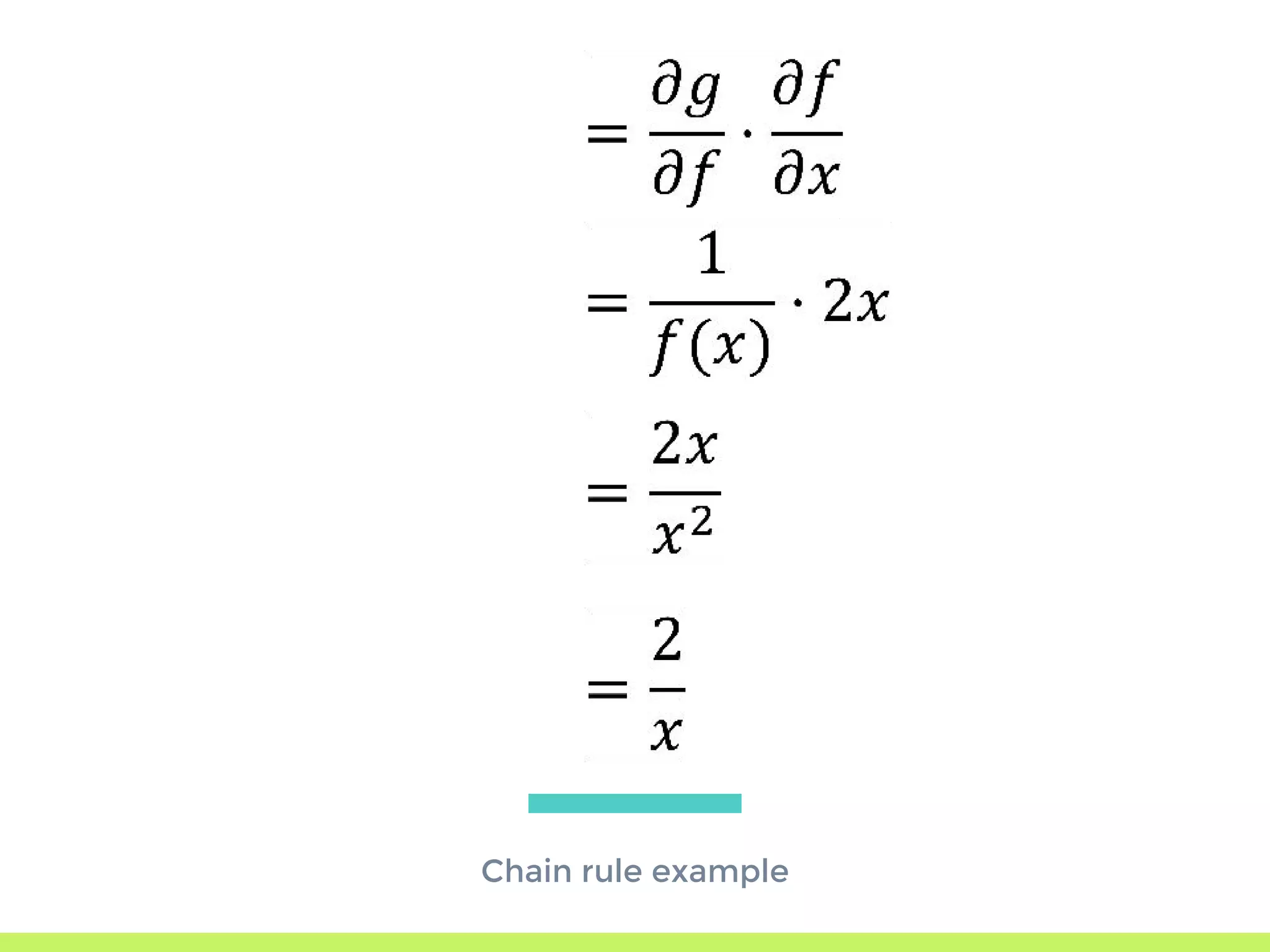
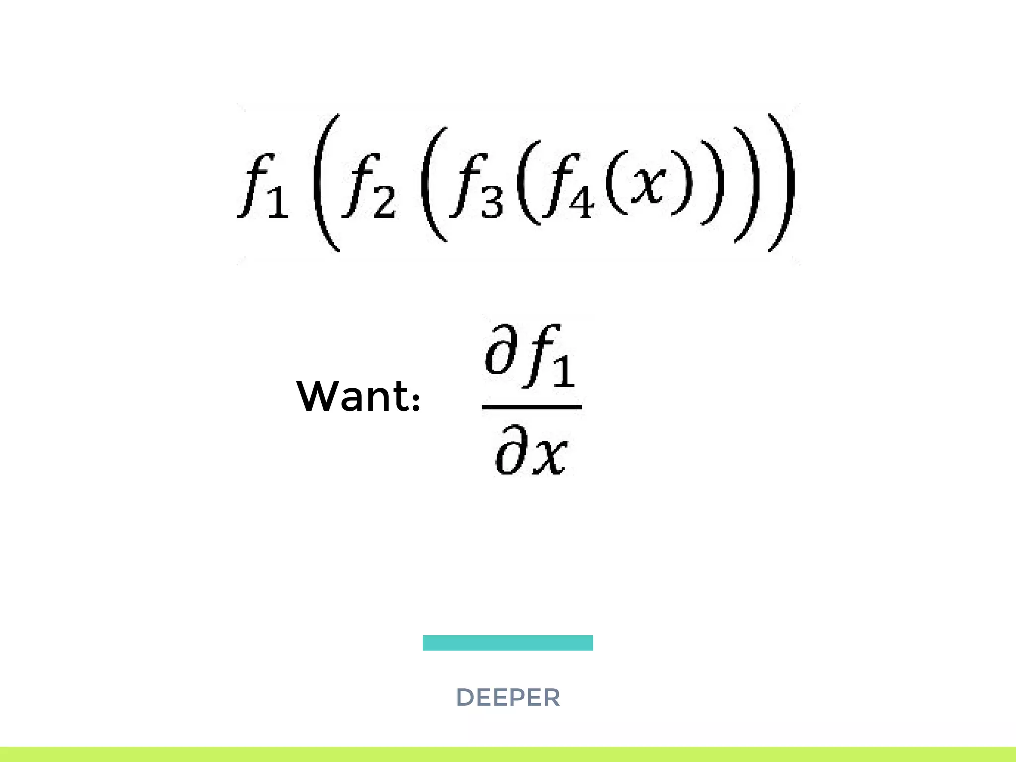
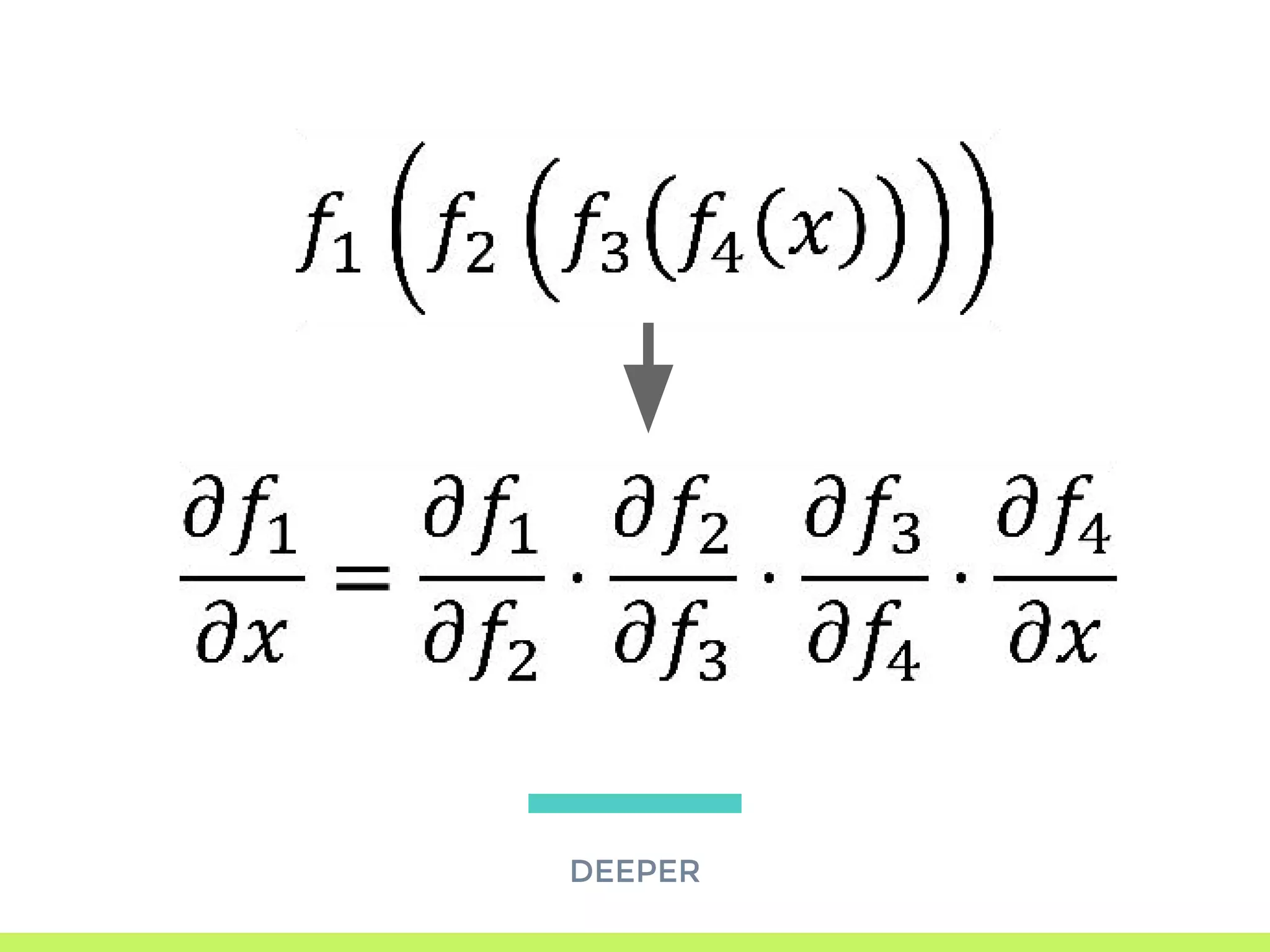
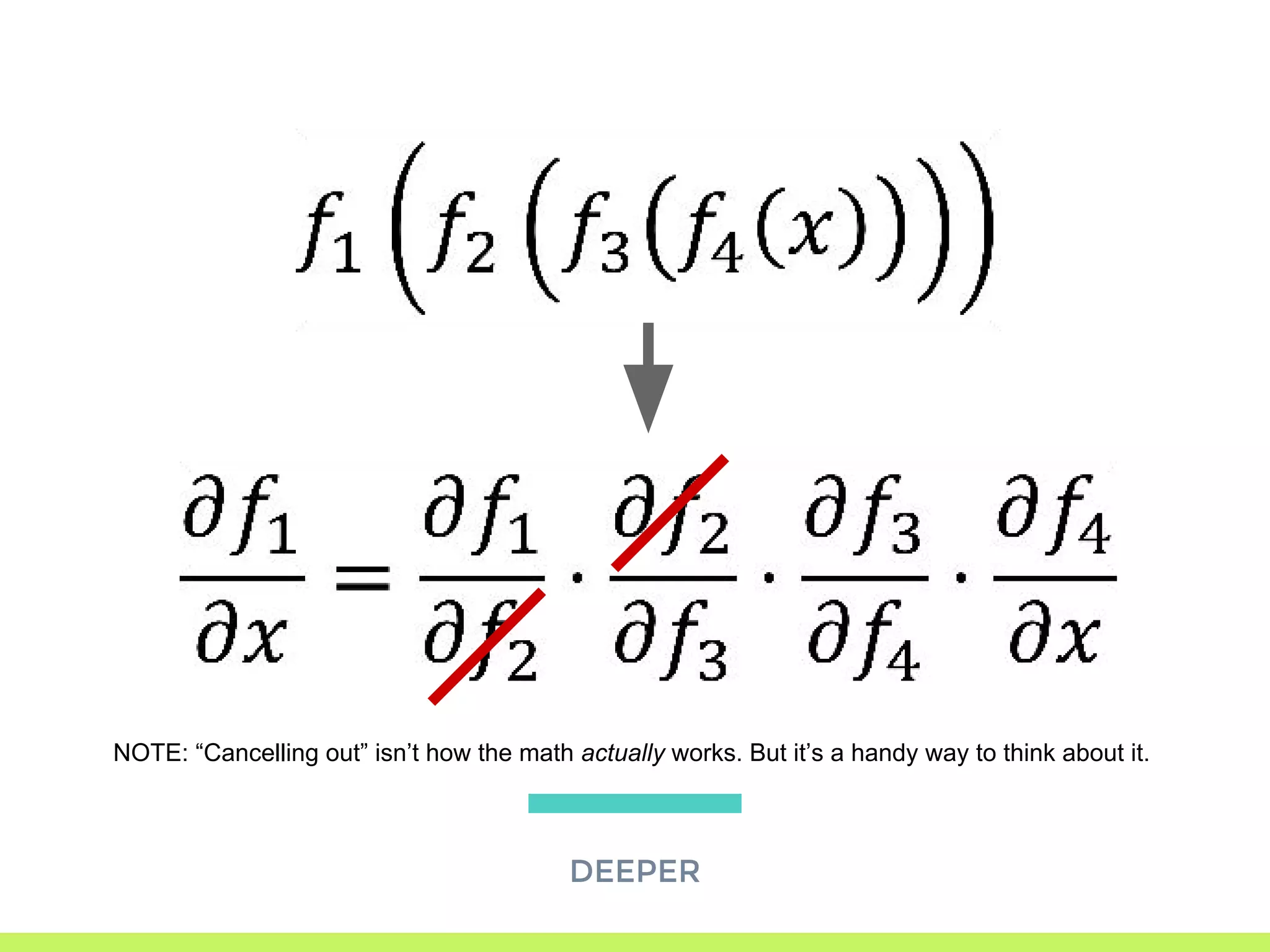
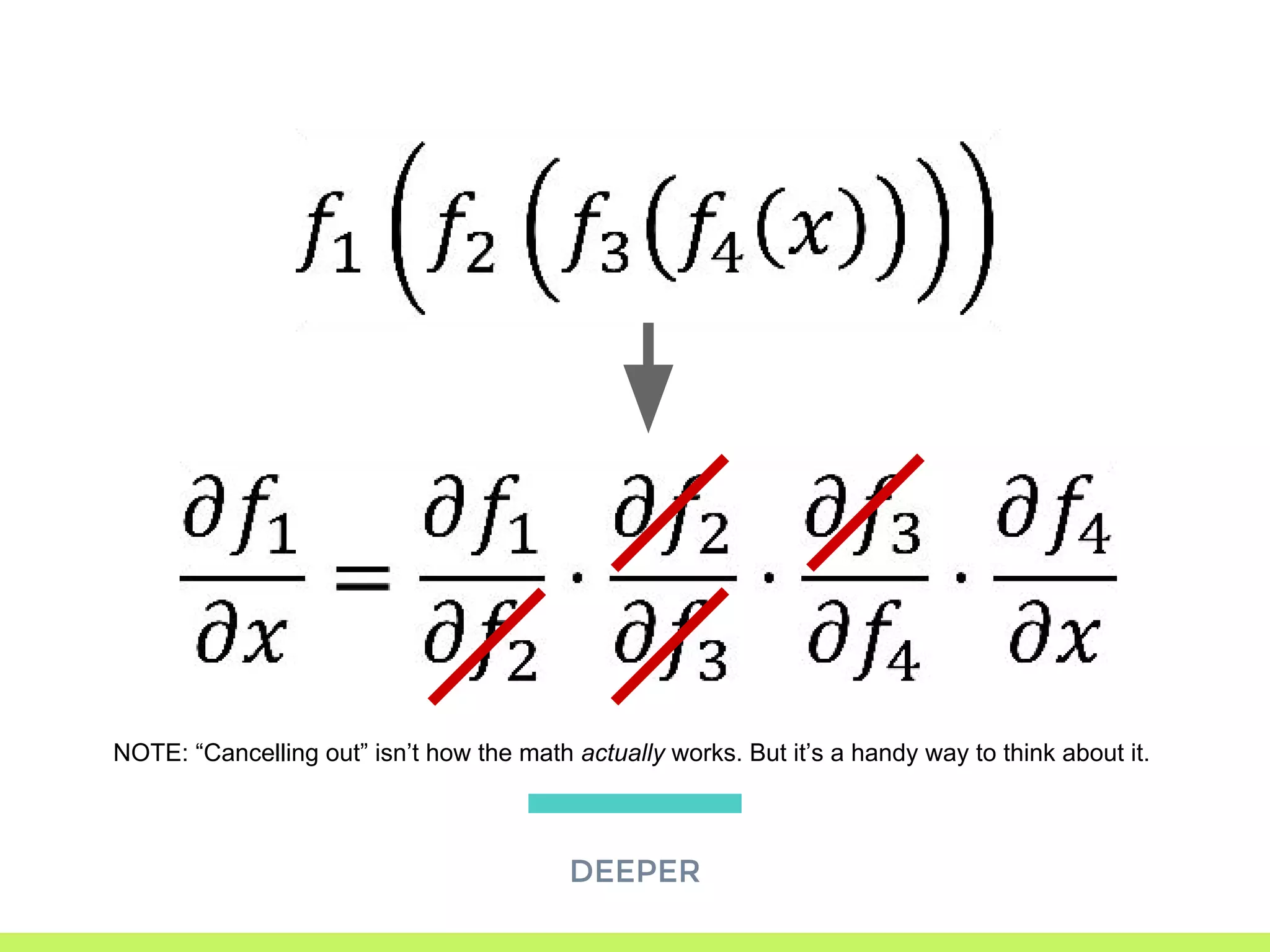
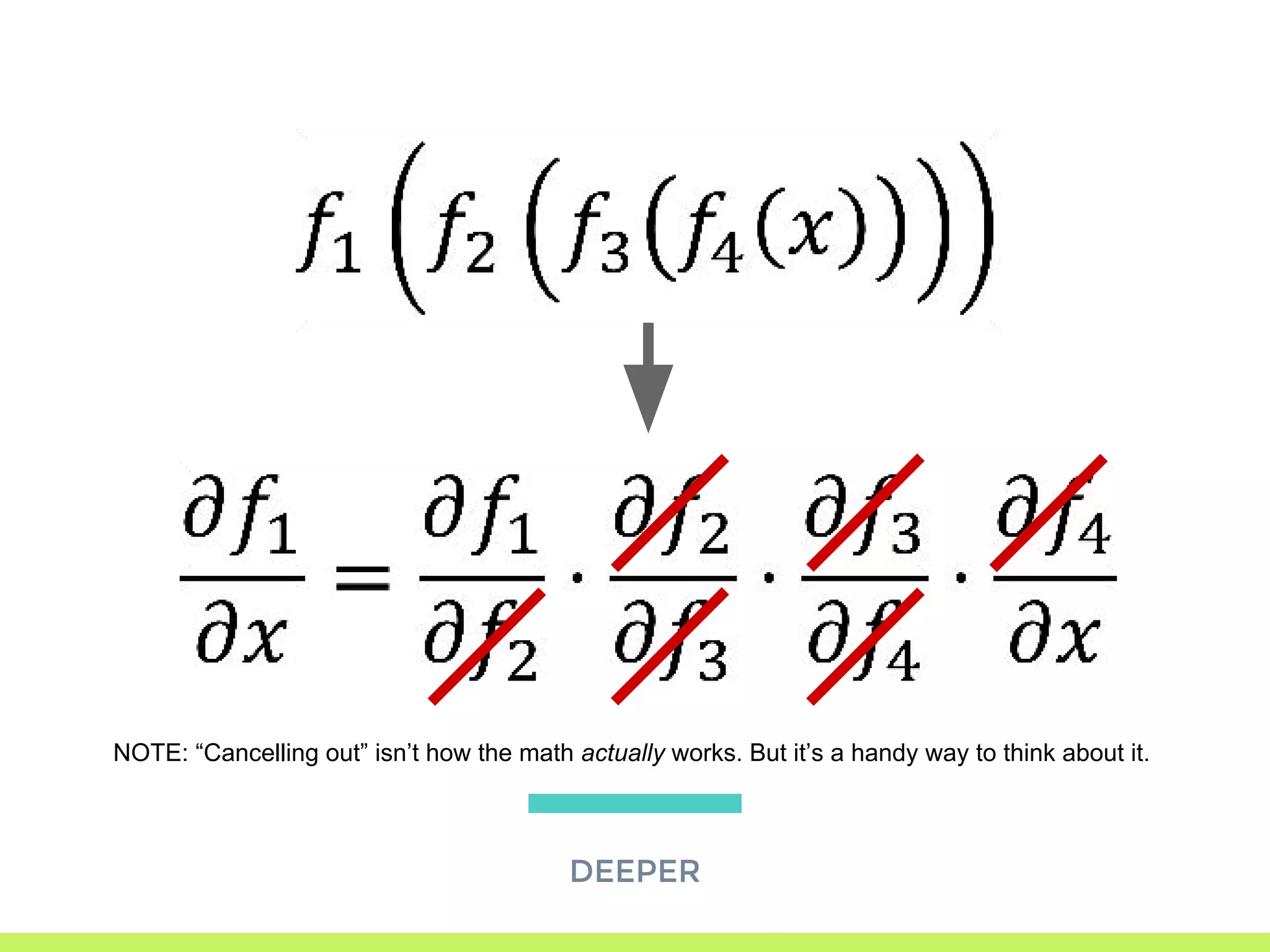
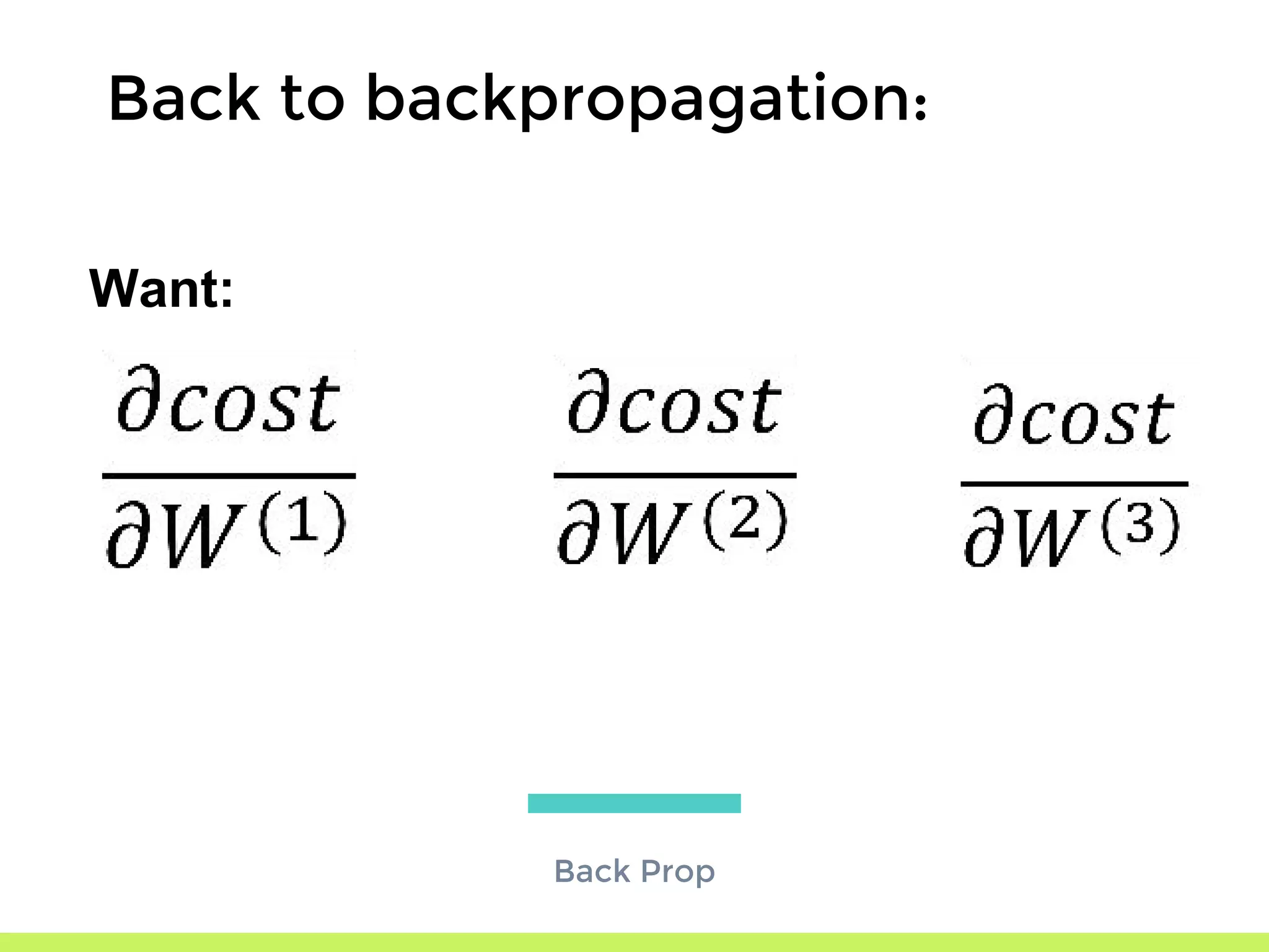
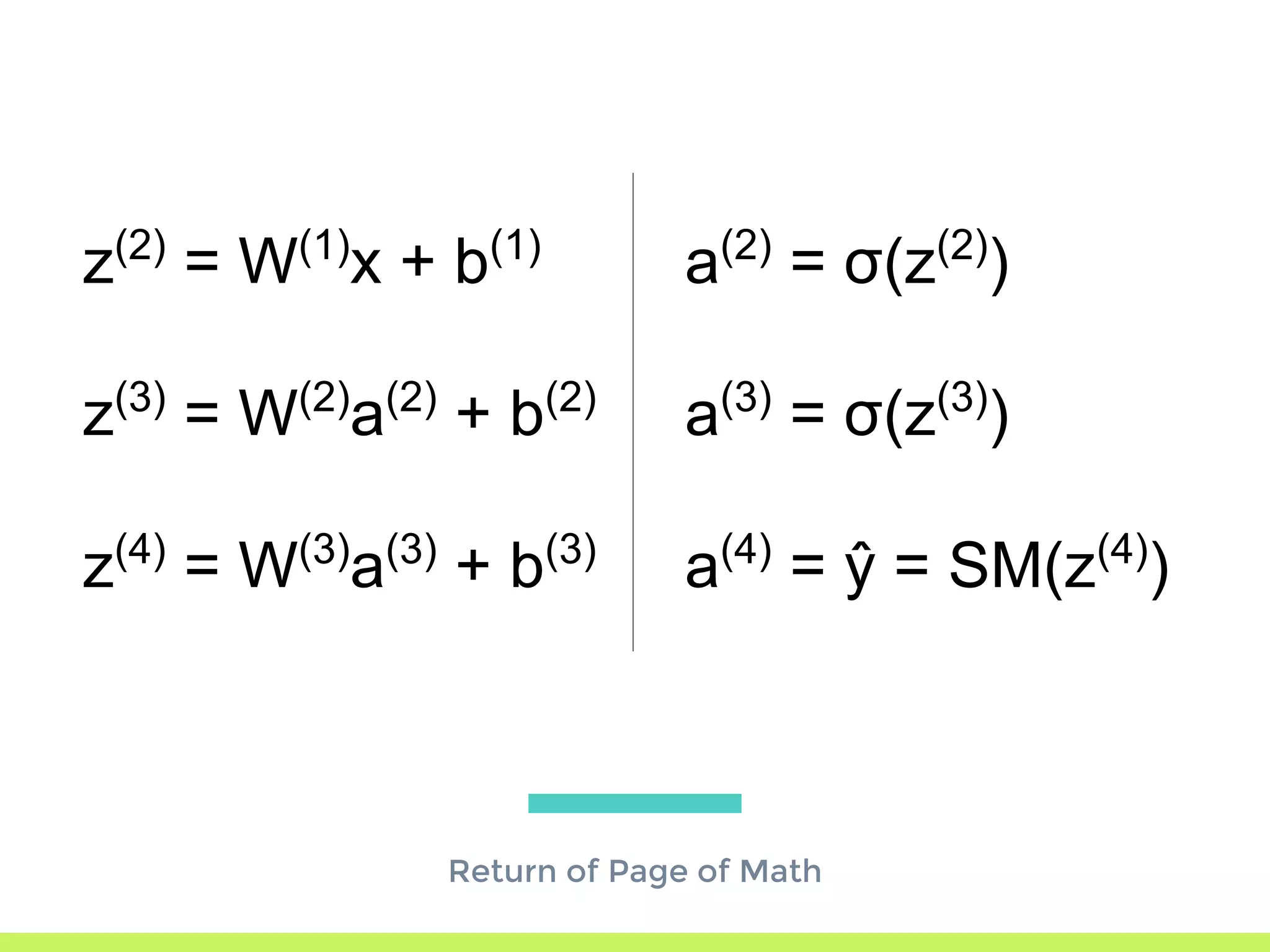
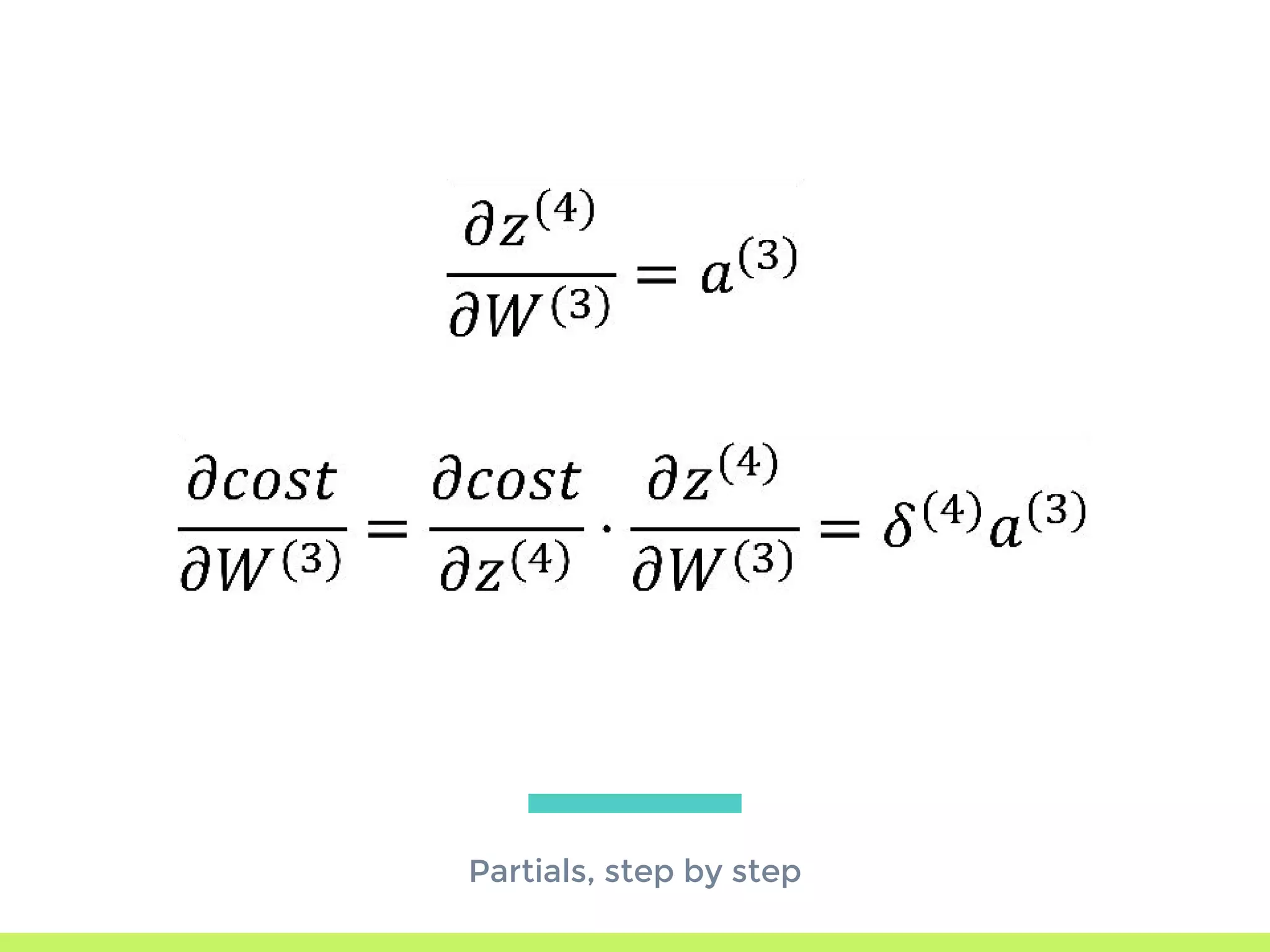
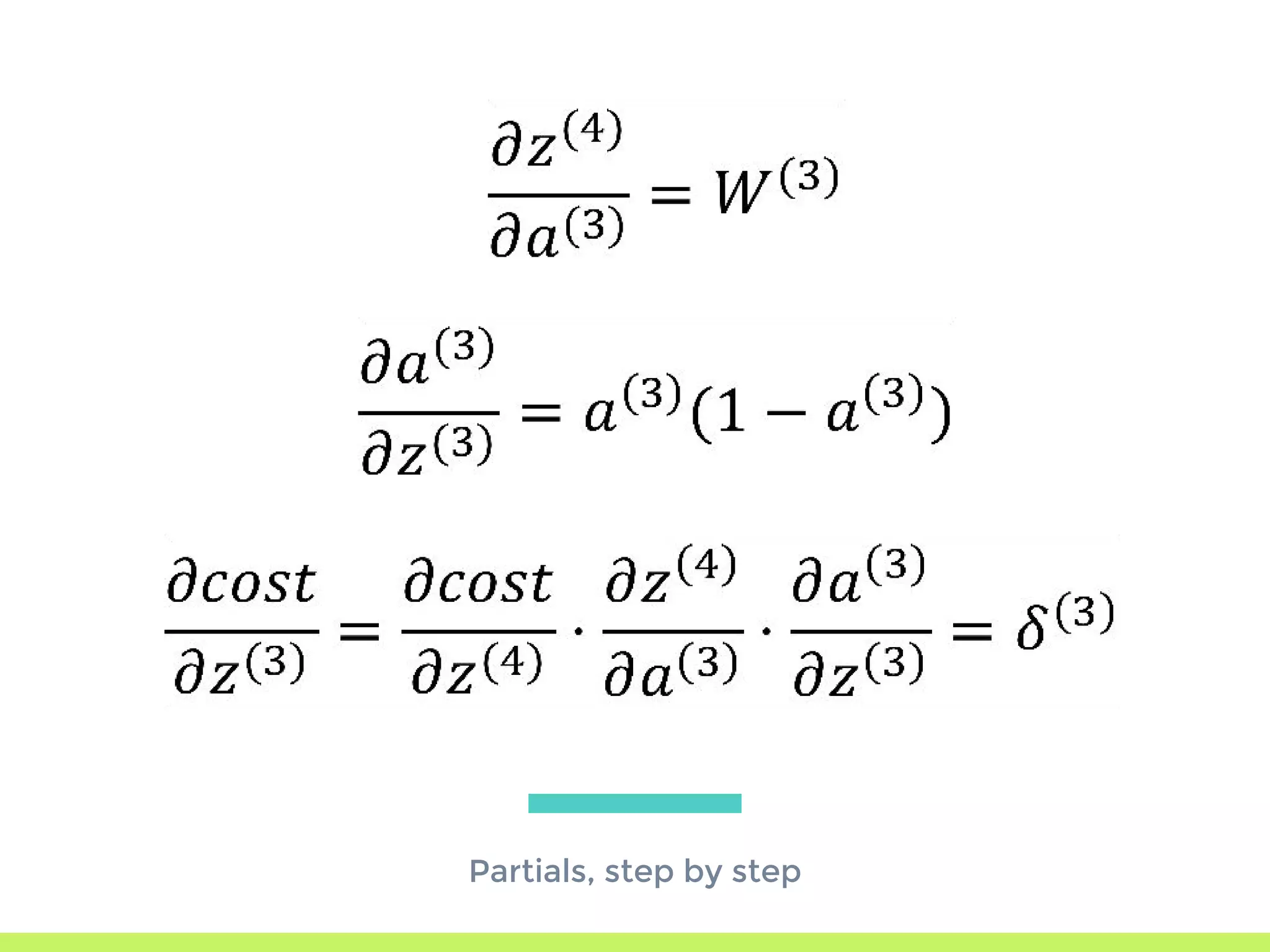
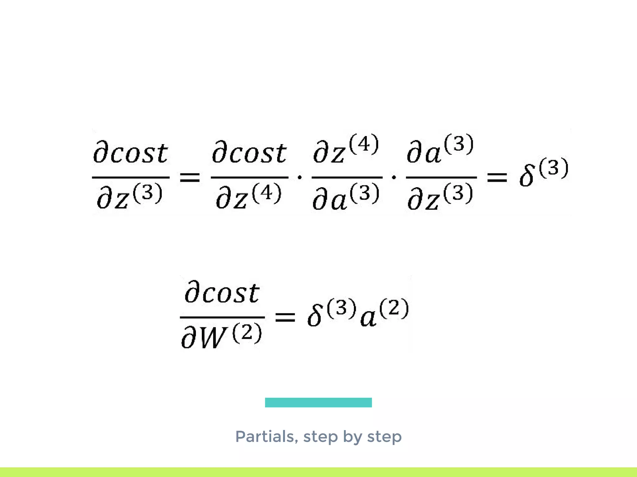
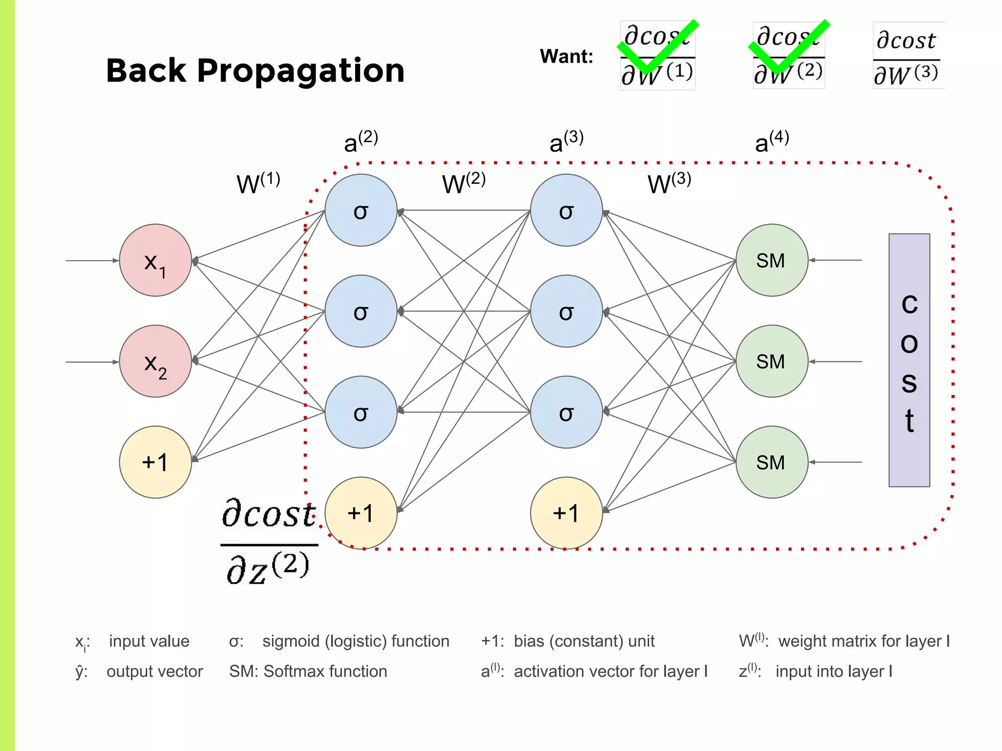
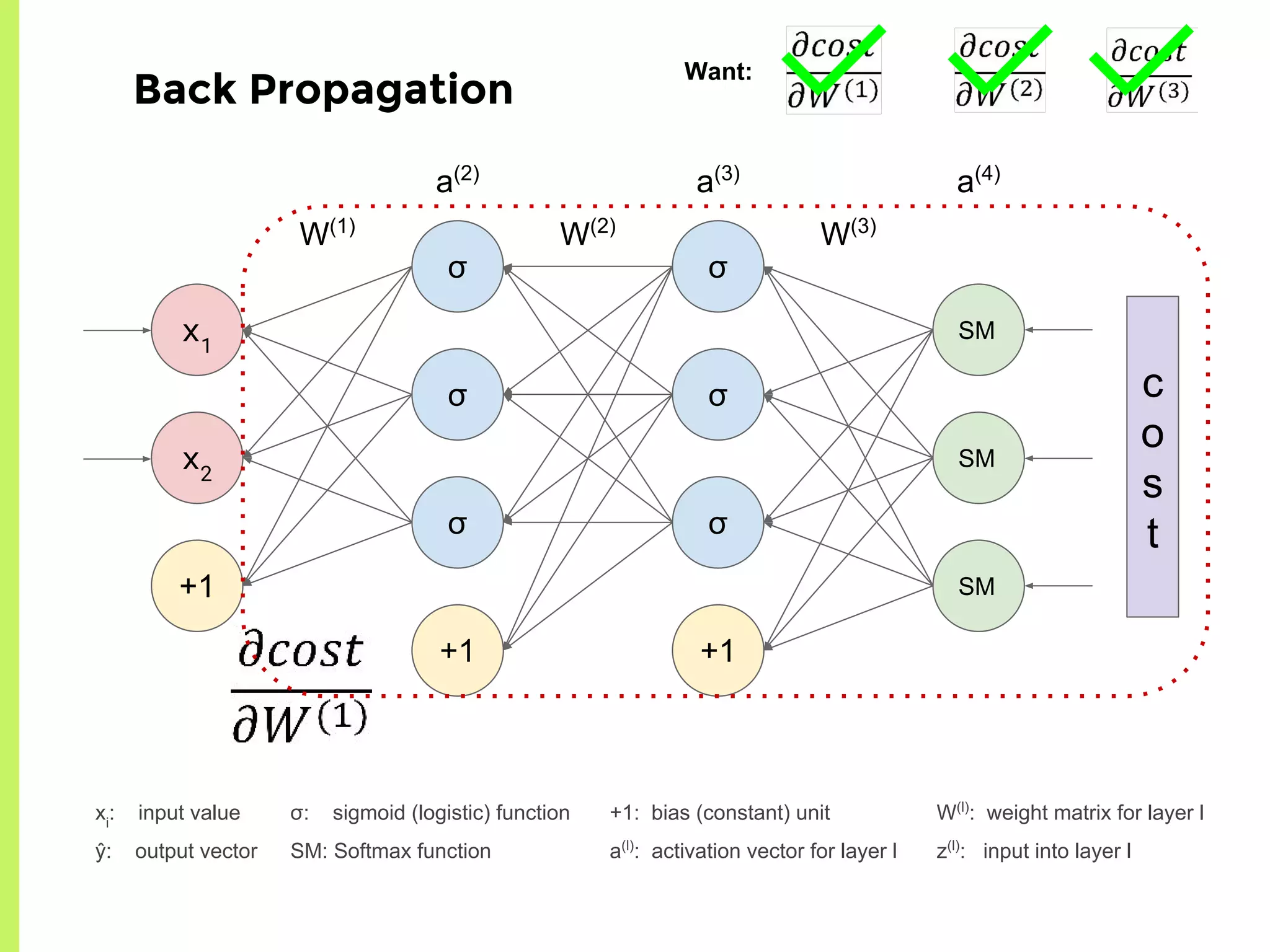
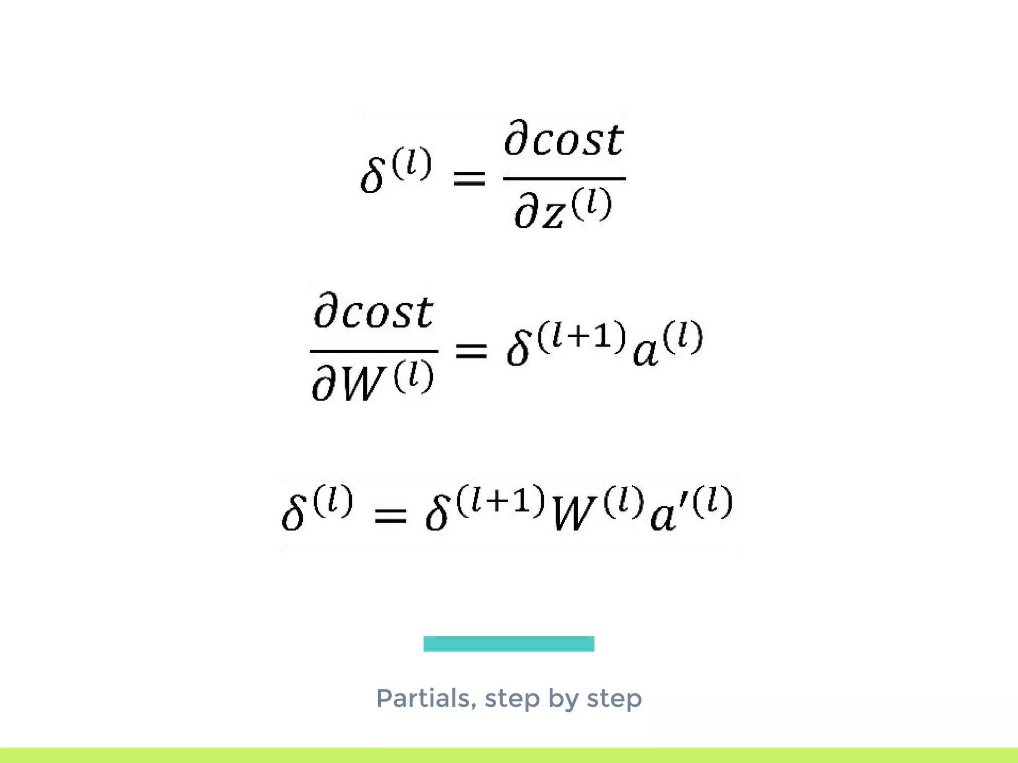
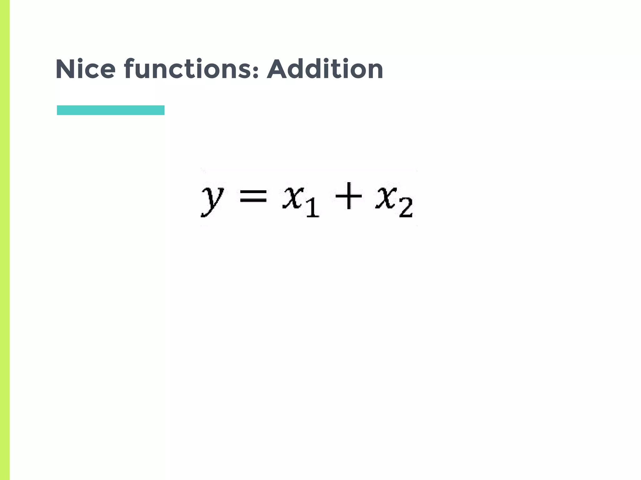
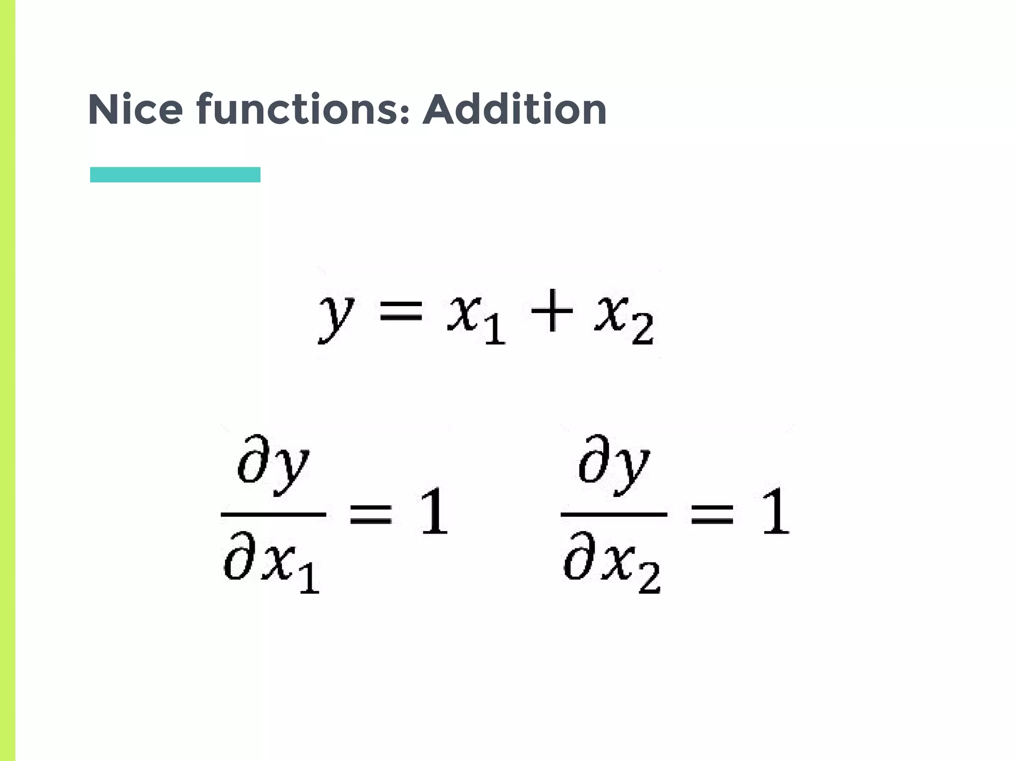
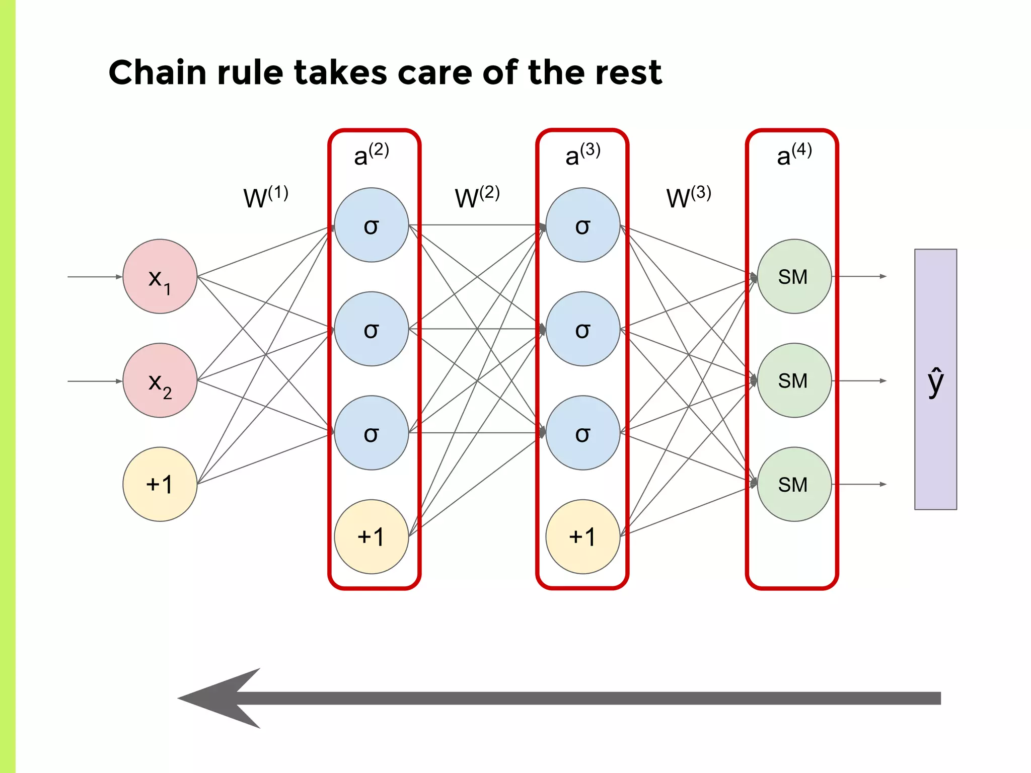
The step-by-step process of forward propagation in a neural network from input to output layer calculations.Detailed explanation of backpropagation, focusing on chain rule and the computation of derivatives in neural networks for training.Introduction to automatic differentiation, its benefits for coding efficiency, and the use of functions that are easy to differentiate.
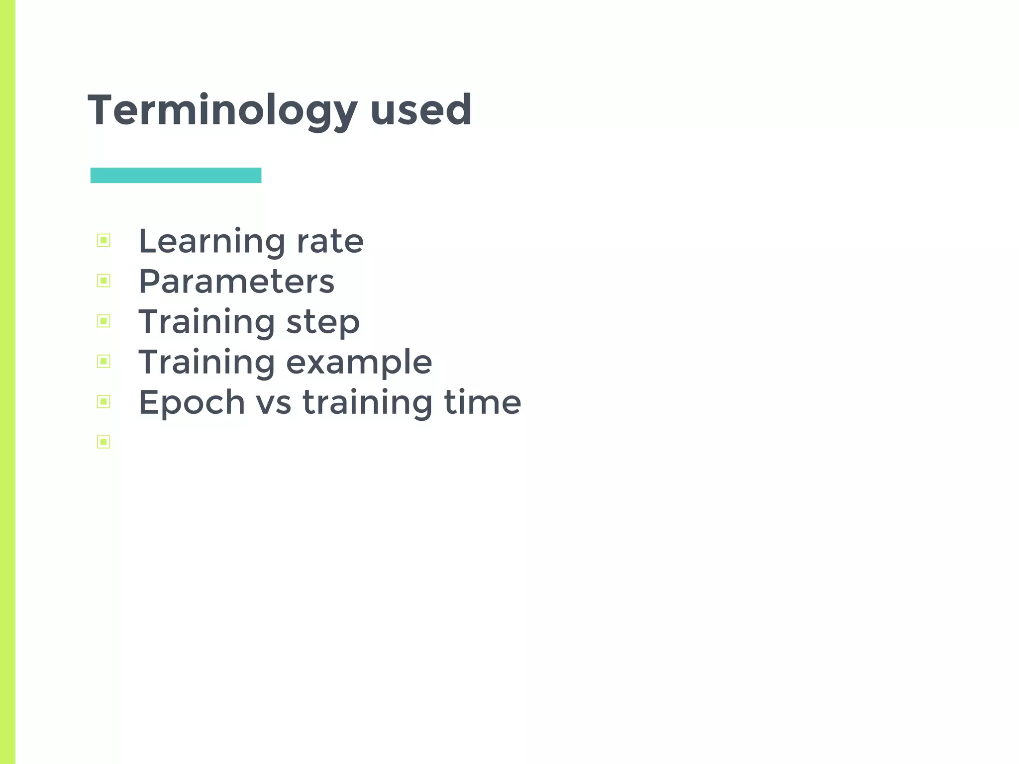
Final slide summarizing the presentation and providing contact information with a glossary of neural network terminology.


![[系列活動] 資料探勘速遊](https://cdn.slidesharecdn.com/ss_thumbnails/0114ycchendmquicktour-170110050658-thumbnail.jpg?width=640&height=640&fit=bounds)


![[DSC 2016] 系列活動:李泳泉 / 星火燎原 - Spark 機器學習初探](https://cdn.slidesharecdn.com/ss_thumbnails/sparkmllib-161026052038-thumbnail.jpg?width=640&height=640&fit=bounds)