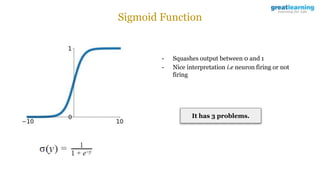
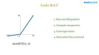
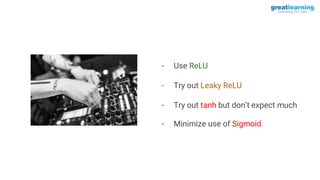
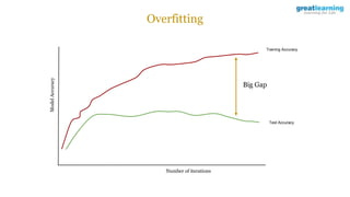
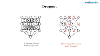
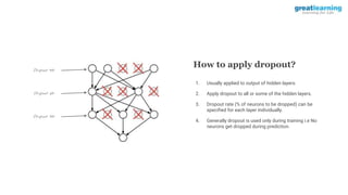
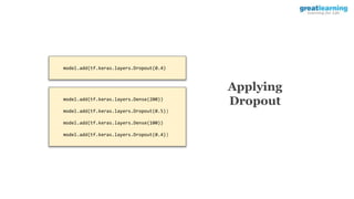
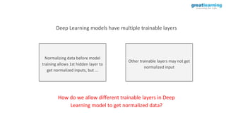
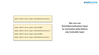
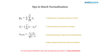
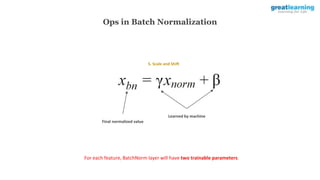
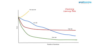
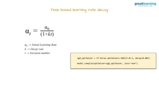
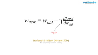
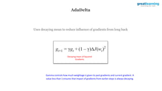
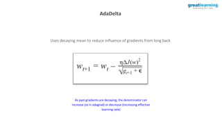
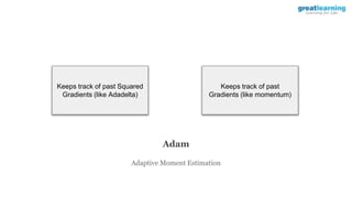
The document discusses different activation functions and their properties for neural networks. It recommends using ReLU or Leaky ReLU activation functions to avoid problems with vanishing gradients in sigmoid and tanh functions. Batch normalization is described as a technique to normalize layer inputs in deep learning models. Dropout is explained as a way to reduce overfitting by randomly dropping neurons during training. Learning rate schedules and optimization algorithms like momentum, Nesterov momentum, Adagrad, and AdaDelta are covered as techniques for improving convergence during training.

1. Activation
Function

2. Controls Neuron’s Output Controls Neuron’s Learning

3. Sigmoid Function
- Squashes output between 0 and 1
- Nice interpretation i.e neuron firing or not
firing
It has 3 problems.

4. Sigmoid Function
Problem 1
- Vanishing Gradient
Derivative is zero when x> 5 or x <-5
- Weights will not change
- No Learning

5. Sigmoid Function
Problem 2
- Output is not Zero-centered
Only positive numbers to Next layer

6. Sigmoid Function
Problem 3
- ey is compute expensive

7. tanh
1. Zero-centered
2. Vanishing gradient
3. Compute expensive
hyperbolic tangent

8. Rectified Linear Unit (ReLU)
1. Does not kill gradient (x>0)
2. Compute inexpensive
3. Converges faster
4. No Zero-centered output

9. Leaky ReLU
1. Does not kill gradient
2. Compute inexpensive
3. Converges faster
4. Somewhat Zero-centered

10. Which activation function we should
use?

11. - Use ReLU
- Try out Leaky ReLU
- Try out tanh but don’t expect much
- Minimize use of Sigmoid

12. Learning
vs
Memorizing

13. How do we know machine is really
learning or memorizing?
By looking at test accuracy (or loss) and
comparing it with training accuracy/loss.

14. Overfitting
Training Accuracy
Number of iterations
Model
Accuracy
Test Accuracy
Big Gap

15. How do we avoid overfitting?
By getting more data, we can make machine
reduce overfitting. But quite often it's not easy to
get additional data.

16. Dropout
...refers to dropping or ignoring
neurons at random to reduce
overfitting.

17. Dropout
A regular Dense
Neural Network
Dense neural network
with ‘Dropout’

18. How to apply dropout?
Dropout 50%
Dropout 60%
Dropout 40%
1. Usually applied to output of hidden layers.
2. Apply dropout to all or some of the hidden layers.
3. Dropout rate (% of neurons to be dropped) can be
specified for each layer individually.
4. Generally dropout is used only during training i.e No
neurons get dropped during prediction.

19. Applying
Dropout
model.add(tf.keras.layers.Dropout(0.4)
model.add(tf.keras.layers.Dense(200))
model.add(tf.keras.layers.Dropout(0.5))
model.add(tf.keras.layers.Dense(100))
model.add(tf.keras.layers.Dropout(0.4))

20. Batch
Normalization

21. How do we normalize data?
There are two approaches which are
common in Machine Learning

22. 1. Min-Max Scaler
Feature value is between 0 and 1 after normalization

23. 2. z-Score Normalization
Mean is 0 and Variance is 1 after normalization

24. When do we normalize data in ML?
We usually normalize the data and
then feed it to the model for training.

25. Deep Learning models have multiple trainable layers
Normalizing data before model
training allows 1st hidden layer to
get normalized inputs, but ...
Other trainable layers may not get
normalized input
How do we allow different trainable layers in Deep
Learning model to get normalized data?

26. Batch Normalization
Implementing data normalization for deeper trainable layers

27. We can use
BatchNormalization layer
to normalize data before
any trainable layer
model.add(tf.keras.layers.BatchNormalization())
model.add(tf.keras.layers.Dense(200))
model.add(tf.keras.layers.BatchNormalization())
model.add(tf.keras.layers.Dense(100))
model.add(tf.keras.layers.BatchNormalization()

28. What type of normalization will
BatchNorm layer do?
z-Score Normalization

29. Ops in Batch Normalization
1. Calculate mean or average for each feature in a batch
2. Calculate Variance for each feature in the batch
3. Normalize each feature using mean and standard deviation
4. Adjust average and variance for a feature across batches
For each feature, BatchNorm layer will calculate two parameters i.e mean and variance

30. So BatchNorm layer works exactly like
a z-Score normalization?
Well, not exactly!
It also allows machine to further modify the normalized
feature value using two learnable parameters.

31. 5. Scale and Shift
Ops in Batch Normalization
Learned by machine
Final normalized value
For each feature, BatchNorm layer will have two trainable parameters.

32. Where to use BatchNorm?
1. Apply it before a trainable layer.
2. Apply it to all or some of the trainable layers.
3. Significant impact on reducing overfitting.
4. Can be used with or inplace of Dropout
Use BatchNorm as much as possible to improve
your Deep neural networks.

33. Learning Rate

34. What is a good learning rate?

35. Very high rate
Low rate
High rate
Good rate
Number of iterations
Loss
Visualizing
Learning Rate

36. Learning
rate decay

37. We usually reduce learning rate as model training progresses to reduce chances of missing minima.

38. Time based learning rate decay
sgd_optimizer = tf.keras.optimizers.SGD(lr=0.1, decay=0.001)
model.compile(optimizer=sgd_optimiser, loss='mse’)

39. Optimizers

40. Stochastic Gradient Descent (SGD)
Key to improving machine’s learning
Learning
Rate

41. Sometimes
it may not
work well...

42. Loss function is
usually quite complex
W
Loss
Let’s review on how Gradient
Descent will change ‘W’ for this
scenario

43. Loss function is
usually quite complex
W
Loss
Let’s review on how Gradient
Descent will change ‘W’ for this
scenario
Starting
position
Gradient Descent will
increase W to reduce loss
. . . reduce ‘w’ again
. . . reduce ‘w’ again
What happens at this point?

44. Loss function is
usually quite complex
W
Loss
Let’s review on how Gradient
Descent will change ‘W’ for this
scenario
Starting
position
Gradient Descent will
increase W to reduce loss
. . . reduce ‘w’ again
. . . reduce ‘w’ again
What happens at this point?
‘W’ does not increase as
Gradient is positive

45. W
Loss Starting
position
Gradient Descent will
increase W to reduce loss
. . . reduce ‘w’ again
. . . reduce ‘w’ again
What happens at this point?
‘W’ does not increase as
Gradient is positive
Problem with SGD
- SGD will get stuck
- Can not find better local minima
- Such scenarios quite common DNNs

46. W
Loss
What happens at this point?
- Zero gradient
- SGD gets stuck
Another scenario
Saddle point

47. How do we overcome local minima &
saddle points?
Bringing Physics to ML

48. Momentum
Using physics in ML
When a ball rolls down the hill …
● it gains in momentum due to gravity.
● ball moves faster and faster .
● Can overcome small hurdles
We can use similar approach in ML to
change weights and bias.

49. How do we use momentum with
weight changes?

50. W
Loss
Starting
position
GD will increase W to
reduce loss
Amount of change in W for
step 1
Step 1
Let’s take an example

51. W
Loss
Starting
position
Change in W without
momentum
Amount of change in W for step 2
with momentum
Step 2
A percent (say 90%)
of change from step 1
Change in W with
momentum

52. W
Loss
Starting
position Amount of change in W for step 3
with momentum
Step 3
A percent (say 90%) of
change from step 2
Change in W with
momentum

53. W
Loss
Starting
position Amount of change in W for step 4
with momentum
Step 4
Although gradient is ‘+’ at
step 4 but gradient from
previous step will allow
machine to increase ‘W’
Change in W with
momentum

54. Momentum
Time step 1
Time step 2
Time step 3
Time step 4
Gradients from all the past steps (in
addition to current step) are used to
calculate final gradient at a step.

55. SGD with Momentum
Gradient
with
Momentum
New
weight
momentum

56. sgd = tf.keras.optimizers.SGD(lr=0.03, momentum=0.9)
Implementing
SGD with Momentum

57. What happens to Saddle point and
local minima?
Momentum gain will allow machine to
overcome these scenarios

58. Can that be a problem?
Momentum ‘may’ allow machine to go
too far away from minima from where it
can not come back

59. How do we overcome such
situations?
If we are coming down a hill, we gain momentum because
of gravity.
● But as we get closer to our destination, we try to
reduce speed not to overshoot our destination.
● We can take action as we are able to see what’s
coming up.

60. Can Machine check
what’s in future?
This means to check if
loss will increase or
decrease in future...

61. How do Check change in loss in
future?
By calculating Loss gradient w.r.t to future
weight

62. How to get future weight?
Gives us some idea about future i.e what will
be the weight at the following step (at t+2)

63. SGD with Nesterov Momentum
Adjusted
Momentum
Gradient of loss is not calculated wrt wt.
Rather, loss gradient is calculated wrt to ‘wt - ४vt-1 ’
i.e future weight

64. sgd = tf.keras.optimizers.SGD(lr=0.03, momentum=0.9, nesterov=True)
Implementing
SGD with Nesterov Momentum
SGD with Nesterov momentum and learning rate decay is a very popular
optimizers to train modern architectures.

65. We use same learning rate all
the weights

66. W1
Loss
W2
Loss
A weight with much faster change in Loss
Another weight with much slower change in Loss

67. W1
Loss
W2
Loss
A weight with much faster change in Loss
Another weight with much slower change in Loss
For this weight, we can apply a higher
learning rate to change W with higher
amount to speed up the learning
Here, it might be better to reduce
amount of changes to ‘W’ by reducing
the learning rate

68. How do use different learning rates for
different weights?
We can use gradient values of the past step
...but in a different way then momentum

69. How should we measure past gradients?
Add Squared Gradient to past Gradients
If a weight has faster loss
change...i.e higher gradients in the
past then this term will be HIGH
If a weight has slower loss
change...i.e smaller gradients in the
past then this term will be LOW

70. Adagrad
Adapts or changes learning rate for each weight
Learning Rate is different at each step for each
weight
Use gt+1 to calculate effective learning rate

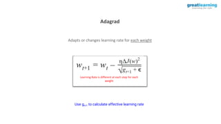
71. model.compile(optimizer=’adagrad’, loss=. . ., metrics=[‘accuracy’])
Implementing Adagrad

72. Adagrad
Advantage
No need to adjust Learning
Rate
Disadvantage
Learning Rate is always
decaying

73. W1
Loss
Consider this scenario

74. How do we avoid always decaying
learning rate in Adagrad?
Do not consider gradients for all the past steps… rather
focus more on recent ones. ..
● If in the recent past gradients were high then
learning rate will be low
● If later, the gradients reduce then we can use
higher learning rate (for the same weight)

75. AdaDelta
Uses decaying mean to reduce influence of gradients from long back
Decaying mean of Squared
Gradients
Gamma controls how much weightage is given to past gradients and current gradient. A
value less than 1 ensures that impact of gradients from earlier steps is always decaying.

76. AdaDelta
Uses decaying mean to reduce influence of gradients from long back
As past gradients are decaying, the denominator can
increase (as in adagrad) or decrease (increasing effective
learning rate)

77. Anything else we can do?
Using approach of both momentum and
Adadelta together . . .

78. Adam
Adaptive Moment Estimation
Keeps track of past Squared
Gradients (like Adadelta)
Keeps track of past
Gradients (like momentum)

79. Calculate Gradient
Decaying mean of past Gradients
(First Moment)
Bias-corrected First moment
Adam
Tracking decaying mean of past gradients

80. Second moment, past squared Gradients
Bias-corrected Second
moment
New Weight
Adam
Tracking decaying mean of past squared gradients

81. New Weight
Adam

82. Adam
Advantage
Removes the need to tune Learning rate
(just set an initial learning rate)
Adam (along with SGD with momentum) is top choice for optimizers in Deep Learning

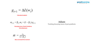
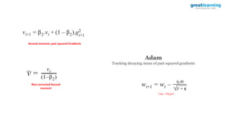
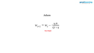
83. model.compile(optimizer=’adam’, loss=’categorical_crossentropy’, metrics=[‘accuracy’])
Implementing Adam

84. 1. Adam
2. SGD with nesterov momentum
3. RMSProp or Adadelta
4. Adagrad
5. Vanilla SGD
Which Optimizer to prefer?

85. Hyperparameters
in
Deep Learning

86. # of iterations Batch Size Learning Rate
# of Hidden Layers # of Neurons in each Layer Activation functions
Learning
rate decay
Dropout Optimizers
Batch Normalization