Downloaded 208 times


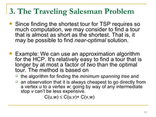
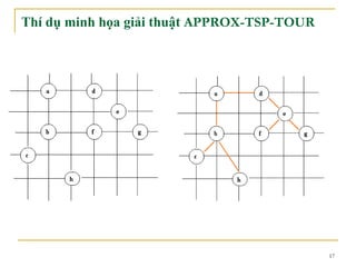
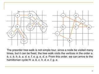
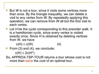
![APPROX-TSP-TOUR The algorithm computes a near-optimal tour of an undirected graph G. procedure APPROX-TSP-TOUR(G, c); begin select a vertex r V[G] to be the “root” vertex; grow a minimum spanning tree T for G from root r, using Prim’s algorithm; apply a preorder tree walk of T and let L be the list of vertices visited in the walk; form the halmintonian cycle H that visits the vertices in the order of L. /* H is the result to return * / end A preorder tree walk recursively visits every vertex in the tree, listing a vertex when its first encountered, before any of its children are visited.](https://image.slidesharecdn.com/chap8new-110820050001-phpapp02/85/Giao-trinh-Phan-tich-va-thi-t-k-gi-i-thu-t-CHAP-8-16-320.jpg)
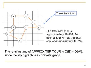
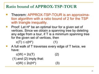

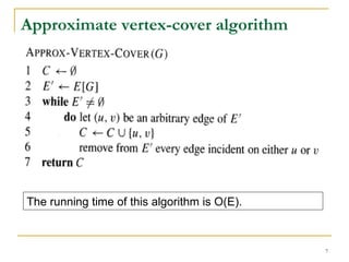
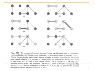
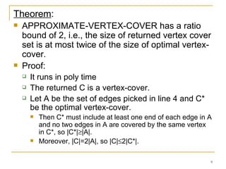
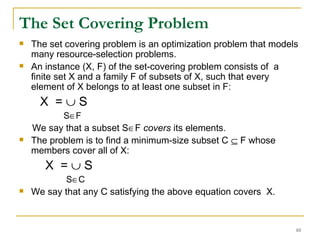
The document outlines approximation algorithms for NP-hard problems including vertex cover, set cover, and traveling salesman problem (TSP). It discusses why approximation algorithms are useful for intractable but important problems. For vertex cover, it presents a 2-approximation algorithm and proves its performance ratio. For set cover, it presents the greedy algorithm and proves its bound of O(ln|X|). For TSP, it presents an algorithm that returns a tour within a factor of 2 the optimal using minimum spanning trees.