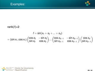
The document discusses the use of low-rank tensor train formats for uncertainty quantification in various computational problems, particularly in numerical aerodynamics. It covers the Karhunen-Loève expansion, polynomial chaos expansions, and tensor train decompositions to efficiently manage uncertainties in input parameters and solutions. The proposed methods aim to enhance the reliability of predictions made by complex computational algorithms.

1. Response Surface in low-rank Tensor Train
Format for Uncertainty Quantification
Alexander Litvinenko1
(joint work with Sergey Dolgov2, Boris Khoromsij2 and
Hermann G. Matthies3)
1 KAUST, 2 Max-Planck-Institut f¨ur Mathematik in den
Naturwissenschaften, Leipzig,
3 Technische Universit¨at Braunschweig, Germany
Center for Uncertainty
Quantification
ntification Logo Lock-up
http://sri-uq.kaust.edu.sa/

2. 4*
Overview of uncertainty quantification
Consider
A(u; q) = f ⇒ u = S(f; q),
where S is a solution operator.
Uncertain Input:
1. Parameter q := q(ω) (assume moments/cdf/pdf/quantiles
of q are given)
2. Boundary and initial conditions, right-hand side
3. Geometry of the domain
Uncertain solution:
1. mean value and variance of u
2. exceedance probabilities P(u > u∗)
3. probability density functions (pdf) of u.
Center for Uncertainty
Quantification
ation Logo Lock-up
2 / 41

3. 4*
Motivation
Nowadays computational algorithms, run on
supercomputers, can simulate and resolve very
complex phenomena. But how reliable are these
predictions? Can we trust to these results?
Some parameters/coefficients are unknown,
lack of data, very few measurements →
uncertainty.
Center for Uncertainty
Quantification
ation Logo Lock-up
3 / 41

4. 4*
Example: Realisations of random fields
Center for Uncertainty
Quantification
ation Logo Lock-up
4 / 41

5. What is Quantification of uncertainties ?
A big example:
UQ in numerical aerodynamics
(described by Navier-Stokes + turbulence modeling)
Center for Uncertainty
Quantification
ation Logo Lock-up
5 / 41

6. 4*
Example: uncertainties in free stream turbulence
α
v
v
u
u’
α’
v1
2
Random vectors v1(θ) and v2(θ) model free stream turbulence
Center for Uncertainty
Quantification
ation Logo Lock-up
6 / 41

7. 4*
Example: UQ
Input parameters: assume that RVs α and Ma are Gaussian
with
mean st. dev.
σ
σ/mean
α 2.79 0.1 0.036
Ma 0.734 0.005 0.007
Then uncertainties in the solution (lift force and drag force) are
lift force 0.853 0.0174 0.02
drag force 0.0206 0.003 0.146
Center for Uncertainty
Quantification
ation Logo Lock-up
7 / 41

8. 4*
500 MC realisations of the pressure in dependence on αi and Mai
Center for Uncertainty
Quantification
ation Logo Lock-up
8 / 41

9. 4*
Consider diffusion equation with uncertain coeffs
− div(κ(x, ω) u(x, ω)) = p(x, ω) in G × Ω, G ⊂ R3,
u = 0 on ∂G,
(1)
where κ(x, ω) - conductivity coefficient. Since κ positive,
usually κ(x, ω) = eγ(x,ω).
Center for Uncertainty
Quantification
ation Logo Lock-up
9 / 41

10. Discretisation of stochastic PDE
Center for Uncertainty
Quantification
ation Logo Lock-up
10 / 41

11. 4*
Karhunen-Lo`eve Expansion
The Karhunen-Lo`eve expansion is the series
κ(x, ω) = µk (x) +
∞
i=1
λiki(x)ξi(ω), where
ξi(ω) are uncorrelated random variables and ki are basis
functions in L2(G).
Eigenpairs λi, ki are the solution of
Tki = λiki, ki ∈ L2
(G), i ∈ N, where.
T : L2(G) → L2(G),
(Tu)(x) := G covk (x, y)u(y)dy.
Center for Uncertainty
Quantification
ation Logo Lock-up
11 / 41

12. 4*
KLE eigenfunctions in 2D
Center for Uncertainty
Quantification
ation Logo Lock-up
12 / 41

13. 4*
Problem with Polynomial Chaos Expansion
ξi(ω) ≈
Z
k=0
ak Ψk (θ1, θ2, ..., θM),
where Z = (M+p)!
M!p! or Z = pM:
- EXPENSIVE!
M = 9, p = 2, Z = 55
M = 9, p = 4, Z = 715
M = 100, p = 4, Z ≈ 4 · 106.
How to store and to handle so many coefficients ?
The orthogonality of Ψk enables the evaluation
ak =
< ξΨk >
< Ψ2
k >
=
1
< Ψ2
k >
ξ(θ(ω))Ψk (θ(ω))dP(ω).
(e.g. Ψk are multivariate Hermite polynomials).
Center for Uncertainty
Quantification
ation Logo Lock-up
13 / 41

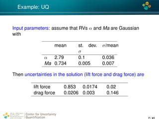
14. 4*
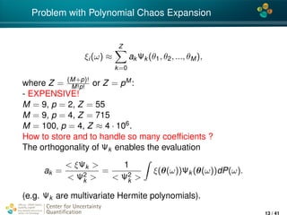
Smooth transformation of Gaussian RF
We assume κ = φ(γ) -a smooth transformation of the Gaussian
random field γ(x, ω), e.g. φ(γ) = exp(γ).
Expanding φ in a series in the Hermite polynomials:
φ(γ) =
∞
i=0
φihi(γ), φi =
+∞
−∞
φ(z)
1
i!
hi(z) exp(−z2
/2)dz, (2)
where hi(z) is the i-th Hermite polynomial.
[see PhD of E. Zander 2013, or PhD of A. Keese, 2005]
Center for Uncertainty
Quantification
ation Logo Lock-up
14 / 41

15. 4*
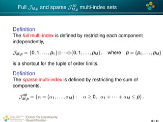
Connection of cov. matrices for κ(x, ω) and γ(x, ω)
First, given the covariance matrix of κ(x, ω), we may relate it
with the covariance matrix of γ(x, ω) as follows,
covκ(x, y) = (κ(x, ω) − ¯κ(x)) (κ(y, ω) − ¯κ(y)) dP(ω)
≈
Q
i=0
i!φ2
i covi
γ(x, y).
Solving this implicit Q-order equation [E. Zander, 13], we derive
covγ(x, y). Now, the KLE may be computed,
γ(x, ω) =
∞
m=1
gm(x)θm(ω),
D
covγ(x, y)gm(y)dy = λmgm(x),
(3)
Center for Uncertainty
Quantification
ation Logo Lock-up
15 / 41

16. 4*
Full JM,p and sparse J sp
M,p multi-index sets
Definition
The full multi-index is defined by restricting each component
independently,
JM,p = {0, 1, . . . , p1}⊗· · ·⊗{0, 1, . . . , pM}, where p = (p1, . . . , pM)
is a shortcut for the tuple of order limits.
Definition
The sparse multi-index is defined by restricting the sum of
components,
J sp
M,p = {α = (α1, . . . , αM) : α ≥ 0, α1 + · · · + αM ≤ p} .
Center for Uncertainty
Quantification
ation Logo Lock-up
16 / 41

17. 4*
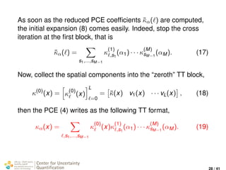
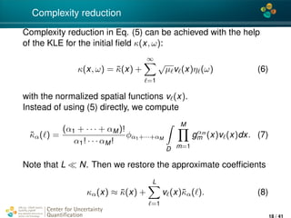
TT compression of PCE coeffs
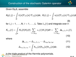
As a result, the M-dimensional PCE approximation of κ writes
κ(x, ω) ≈
α∈JM
κα(x)Hα(θ(ω)), Hα(θ) := hα1
(θ1) · · · hαM
(θM)
(4)
The Galerkin coefficients κα are evaluated as follows [Thm
3.10, PhD of E. Zander 13],
κα(x) =
(α1 + · · · + αM)!
α1! · · · αM!
φα1+···+αM
M
m=1
gαm
m (x), (5)
where φ|α| := φα1+···+αM
is the Galerkin coefficient of the
transform function in (2), and gαm
m (x) means just the αm-th
power of the KLE function value gm(x).
Center for Uncertainty
Quantification
ation Logo Lock-up
17 / 41

18. 4*
Complexity reduction
Complexity reduction in Eq. (5) can be achieved with the help
of the KLE for the initial field κ(x, ω):
κ(x, ω) = ¯κ(x) +
∞
=1
√
µ v (x)η (ω) (6)
with the normalized spatial functions v (x).
Instead of using (5) directly, we compute
˜κα( ) =
(α1 + · · · + αM)!
α1! · · · αM!
φα1+···+αM
D
M
m=1
gαm
m (x)v (x)dx. (7)
Note that L N. Then we restore the approximate coefficients
κα(x) ≈ ¯κ(x) +
L
=1
v (x)˜κα( ). (8)
Center for Uncertainty
Quantification
ation Logo Lock-up
18 / 41

19. 4*
Construction of the stochastic Galerkin operator
Given Eq.6, assemble
K0(i, j) =
D
¯κ(x) ϕi(x)· ϕj(x)dx, K (i, j) =
D
v (x) ϕi(x)· ϕj(x)dx
(9)
for i, j = 1, . . . , N, = 1, . . . , L. Take ˜κα( ) and integrate over θ:
Kα,β( ) =
RM
Hα(θ)Hβ(θ)
γ∈JM,p
κγ( )Hγ(θ)dθ =
γ∈JM,p
∆α,β,γκγ( ),
(10)
where
∆α,β,γ = ∆α1,β1,γ1
· · · ∆αM ,βM ,γM
, (11)
∆αm,βm,γm =
R
hαm (z)hβm (z)hγm (z)dz, (12)
is the triple product of the Hermite polynomials.Center for Uncertainty
Quantification
ation Logo Lock-up
19 / 41

20. 4*
Stochastic Galerkin operator
Putting together (8), (9) and (10), we obtain the whole discrete
stochastic Galerkin operator,
K = K0 ⊗ ∆0 +
L
=1
K ⊗
γ∈JM,p
∆γ ˜κγ( ), (13)
which K ∈ RN(p+1)M ×N(p+1)M
in case of full JM,p.
If ˜κγ is computed in the tensor product format, the direct
product in ∆ (11) allows to exploit the same format for (13), and
build the operator easily.
Center for Uncertainty
Quantification
ation Logo Lock-up
20 / 41

21. 4*
Tensor Train
Two tensor Train examples
Center for Uncertainty
Quantification
ation Logo Lock-up
21 / 41

22. 4*
Examples (B. Khoromskij’s lecture)
f(x1, ..., xd ) = w1(x1) + w2(x2) + ... + wd (xd )
= (w1(x1), 1)
1 0
w2(x2) 1
...
1 0
wd−1(xd−1) 1
1
wd (xd )
Center for Uncertainty
Quantification
ation Logo Lock-up
22 / 41

23. 4*
Examples:
rank(f)=2
f = sin(x1 + x2 + ... + xd )
= (sin x1, cos x1)
cos x2 − sin x2
sin x2 cos x2
...
cos xd−1 − sin xd−1
sin xd−1 cos xd−1
cos xd
sin xd−1
Center for Uncertainty
Quantification
ation Logo Lock-up
23 / 41

24. 4*
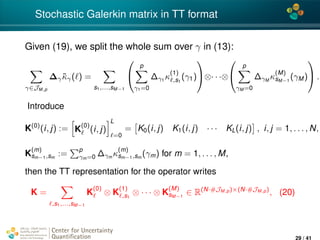
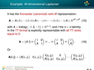
Tensor Train decomposition
u(α) = τ(u(1)
, . . . , u(M)
), meaning
u(α1, . . . , αM) =
r1
s1=1
r2
s2=1
· · ·
rM−1
sM−1=1
u
(1)
s1
(α1)u
(2)
s1,s2
(α2) · · · u
(M)
sM−1
(αM), o
u(α1, . . . , αM) = u(1)
(α1)u(2)
(α2) · · · u(M)
(αM), or
u =
r1
s1=1
r2
s2=1
· · ·
rM−1
sM−1=1
u
(1)
s1
⊗ u
(2)
s1,s2
⊗ · · · ⊗ u
(M)
sM−1
.
(14)
Each TT core u(k) = [u
(k)
sk−1,sk
(αk )] is defined by rk−1nk rk
numbers, where nk is number of grid points (e.g. nk = pk + 1)
in the αk direction, and rk is the TT rank. The total number of
entries O(Mnr2), r = max{rk }.
Center for Uncertainty
Quantification
ation Logo Lock-up
24 / 41

25. 4*
Example: M-dimensional Laplacian
It has the Kronecker (canonical) rank-M representation:
A = A⊗I⊗· · ·⊗I+I⊗A⊗· · ·⊗I+· · ·+I⊗I⊗· · ·⊗A ∈ RnM ×nM
(15)
with A = tridiag{−1, 2, −1} ∈ Rn×n, and I the n × n identity.
In the TT format is explicitly representable with all TT ranks
equal to 2:
A = (A I) 1
I 0
A I
1 ... 1
I 0
A I
1
I
A
, (16)
Or
A(i, j) = A(i1, j1) I(i1, j1)
I(i2, j2) 0
A(i2, j2) I(i2, j2)
· · ·
I(id , jd )
A(id , jd )
.
Center for Uncertainty
Quantification
ation Logo Lock-up
25 / 41

26. 4*
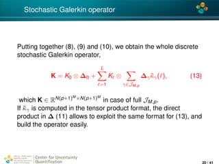
Low-rank response surface: PCE in the TT format
Calculation of
˜κα( ) =
(α1 + · · · + αM)!
α1! · · · αM!
φα1+···+αM
D
M
m=1
gαm
m (x)v (x)dx.
in tensor formats needs:
given a procedure to compute each element of a tensor,
e.g. ˜κα1,...,αM
by (26).
build a TT approximation ˜κα ≈ κ(1)(α1) · · · κ(M)(αM) using
a feasible amount of elements (i.e. much less than
(p + 1)M).
Such procedure exists, and relies on the cross interpolation of
matrices, generalized to a higher-dimensional case [Oseledets,
Tyrtyshnikov 2010; Savostyanov 13; Grasedyck; Bebendorf].
Center for Uncertainty
Quantification
ation Logo Lock-up
26 / 41

27. Skip 3 technical slides about Maximum volume
principle and its application
Center for Uncertainty
Quantification
ation Logo Lock-up
27 / 41

28. As soon as the reduced PCE coefficients ˜κα( ) are computed,
the initial expansion (8) comes easily. Indeed, stop the cross
iteration at the first block, that is
˜κα( ) =
s1,...,sM−1
κ
(1)
,s1
(α1) · · · κ
(M)
sM−1
(αM). (17)
Now, collect the spatial components into the “zeroth” TT block,
κ(0)
(x) = κ
(0)
(x)
L
=0
= ¯κ(x) v1(x) · · · vL(x) , (18)
then the PCE (4) writes as the following TT format,
κα(x) =
,s1,...,sM−1
κ
(0)
(x)κ
(1)
,s1
(α1) · · · κ
(M)
sM−1
(αM). (19)
Center for Uncertainty
Quantification
ation Logo Lock-up
28 / 41

29. 4*
Stochastic Galerkin matrix in TT format
Given (19), we split the whole sum over γ in (13):
γ∈JM,p
∆γ ˜κγ( ) =
s1,...,sM−1


p
γ1=0
∆γ1
κ
(1)
,s1
(γ1)

⊗· · ·⊗


p
γM =0
∆γM
κ
(M)
sM−1
(γM )

 .
Introduce
K(0)
(i, j) := K
(0)
(i, j)
L
=0
= K0(i, j) K1(i, j) · · · KL(i, j) , i, j = 1, . . . , N,
K
(m)
sm−1,sm
:=
p
γm=0 ∆γm
κ
(m)
sm−1,sm
(γm) for m = 1, . . . , M,
then the TT representation for the operator writes
K =
,s1,...,sM−1
K
(0)
⊗ K
(1)
,s1
⊗ · · · ⊗ K
(M)
sM−1
∈ R(N·#JM,p)×(N·#JM,p)
, (20)
Center for Uncertainty
Quantification
ation Logo Lock-up
29 / 41

30. 4*
Post-processing:
We compute
Characteristic, level sets, frequency in TT format
Center for Uncertainty
Quantification
ation Logo Lock-up
30 / 41

31. 4*
Numerics: Main steps
1. Compute PCE of the coefficients κ(x, ω) in TT format
2. Compute stochastic Galerkin matrix K in TT
3. Compute solution of the linear system in TT
4. Post-processing in TT format
Center for Uncertainty
Quantification
ation Logo Lock-up
31 / 41

32. 4*
Numerics: Initial data and software
κ(x, ω) obeys the β{5, 2}-distribution,
covκ(x, y) = exp −(x − y)2/σ2 with σ = 0.3. D is L-shape
domain, 557 DOFs.
Use sglib (E. Zander, TU BS) for discretization and solution with
J sp
M,p.
Use TT-Toolbox for full JM,p.
Use sglib for low-dimensional stages,
and replace high-dimensional calculations by the TT.
Use amen cross.m for TT approximation of ˜κα (26),
Use amen solve.m ( tAMEn, Dolgov) as linear system solver
in TT format.
Center for Uncertainty
Quantification
ation Logo Lock-up
32 / 41

33. 4*
Computation of the PCE for the permeability coefficient
Table : CPU times (sec.) of the permeability assembly
Sparse TT
p M 10 20 30 10 20 30
1 0.2924 0.3113 0.3361 3.6425 68.505 616.97
2 0.3048 0.3556 0.4290 6.3861 138.31 1372.9
3 0.3300 0.5408 1.0302 8.8109 228.92 2422.9
4 0.4471 1.7941 6.4483 10.985 321.93 3533.4
5 1.1291 7.6827 46.682 14.077 429.99 4936.8
Center for Uncertainty
Quantification
ation Logo Lock-up
33 / 41

34. Table : Discrepancies in the permeability coefficients at J sp
M,p
p 1 2 3 4 5
M = 10 2.21e-4 3.28e-5 1.22e-5 4.15e-5 6.38e-5
M = 20 3.39e-4 5.19e-5 2.20e-5 — —
M = 30 5.23e-2 5.34e-2 — — —
Center for Uncertainty
Quantification
ation Logo Lock-up
34 / 41

35. 4*
CPU times (sec.) of the operator assembly
Sparse TT
p M 10 20 30 10 20 30
1 0.1226 0.2171 0.3042 0.1124 0.2147 0.3836
2 0.1485 2.1737 26.510 0.1116 0.2284 0.5438
3 2.2483 735.15 — 0.1226 0.2729 0.8403
4 82.402 — — 0.1277 0.2826 1.0832
5 3444.6 — — 0.2002 0.3495 1.1834
Center for Uncertainty
Quantification
ation Logo Lock-up
35 / 41

36. 4*
CPU times (sec.) of the solution
Sparse TT
p M 10 20 30 10 20 30
1 0.2291 1.169 0.4778 1.074 9.3492 51.177
2 0.3088 2.123 3.2153 1.681 27.014 173.21
3 0.8112 14.04 — 2.731 56.041 391.59
4 5.7854 — — 7.237 142.87 1497.1
5 61.596 — — 45.51 866.07 5362.8
Center for Uncertainty
Quantification
ation Logo Lock-up
36 / 41

37. 4*
Errors in the solution covariance matrices, | covu − covu |
The reference covariance matrix covu ∈ RN×N is computed in
the TT format with p = 5, and the discrepancies in the results
with smaller p are calculated in average over all spatial points,
| covu − covu | =
i,j(covu − covu)2
i,j
i,j(covu)2
i,j
.
Sparse TT
p M 10 20 30 10 20 30
1 9.49e-2 8.86e-2 9.67e-2 4.18e-2 2.80e-2 2.60e-2
2 3.46e-3 2.65e-3 3.34e-3 1.00e-4 1.31e-4 2.12e-4
3 1.65e-4 2.77e-4 — 4.48e-5 1.32e-4 2.14e-4
4 8.58e-5 — — 6.28e-5 1.33e-4 1.11e-4
Center for Uncertainty
Quantification
ation Logo Lock-up
37 / 41

38. 4*
Take to home
1. demonstrated RS in TT format for solving PDEs with
uncertain coefficients.
2. Favor of the TT comparing to CP is a stable quasi-optimal
rank reduction based on SVD.
3. Complexity O(Mnr3) with full accuracy control.
4. TT methods become preferable for high p, but otherwise
the full computation in a small sparse set may be incredibly
fast. This reflects well the “curse of order”, taking place for
the sparse set instead of the “curse of dimensionality” in
the full set: the cardinality of the sparse set grows
exponentially with p.
5. The TT approach scales linearly with p.
Center for Uncertainty
Quantification
ation Logo Lock-up
38 / 41

39. 4*
Take to home
1. TT methods allow easy calculation of the stochastic
Galerkin operator. With p below 10, the TT storage of the
operator allows us to forget about the sparsity issues,
since the number of TT entries O(Mp2r2) is tractable.
2. Other polynomial families, such as the Chebyshev or
Laguerre, may be incorporated into the scheme freely.
3. TT formalism may be recommended for stochastic PDEs
as a general tool: one introduces the same discretization
levels for all variables and let the algorithms determine a
quasi-optimal representation adaptivity.
Center for Uncertainty
Quantification
ation Logo Lock-up
39 / 41

40. 4*
Many questions are still open
1. Can we endow the solution scheme with more structure
and obtain a more efficient algorithm?
2. Is there a better way to discretize stochastic fields than the
KLE-PCE approach?
3. In the preliminary experiments, we have investigated only
the simplest statistics, i.e. mean and variance. What
quantities (level sets, frequency,...) are feasible in TT
format and how can they be effectively computed?
Center for Uncertainty
Quantification
ation Logo Lock-up
40 / 41

41. 4*
Stochastic Galerkin library
1. Type in your terminal
git clone git://github.com/ezander/sglib.git
2. To initialize all variables, run startup.m
You will find:
generalised PCE, sparse grids, (Q)MC, stochastic Galerkin,
linear solvers, KLE, covariance matrices, statistics, quadratures
(multivariate Chebyshev, Laguerre, Lagrange, Hermite ) etc
There are: many examples, many test, rich demos
Center for Uncertainty
Quantification
ation Logo Lock-up
41 / 41