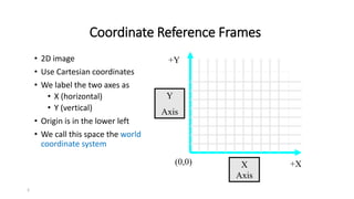
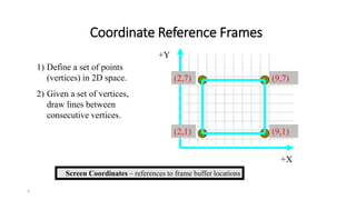
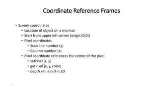
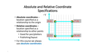
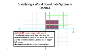
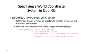
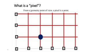
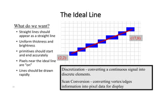
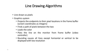
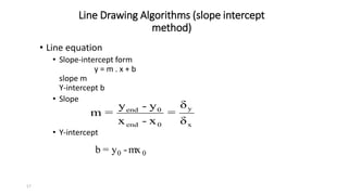
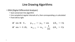
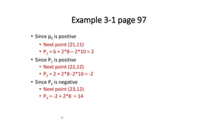
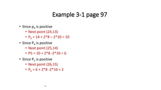
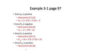
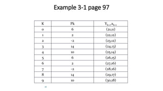
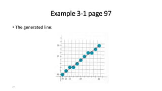
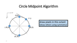
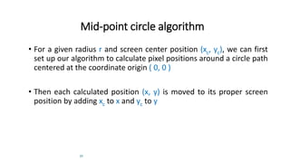
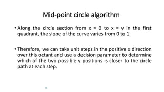
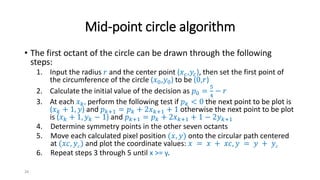
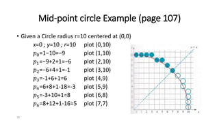
2. Output Primitives
• Graphic SW and HW provide subroutines to describe a scene in terms
of basic geometric structures called output primitives
• Output primitives are combined to form complex structures
• Simplest primitives
• Point (pixel)
• Line segment
2
3. 3
Coordinate Reference Frames
• 2D image
• Use Cartesian coordinates
• We label the two axes as
• X (horizontal)
• Y (vertical)
• Origin is in the lower left
• We call this space the world
coordinate system
X
Axis
Y
Axis
(0,0) +X
+Y
4. 4
Coordinate Reference Frames
1) Define a set of points
(vertices) in 2D space.
2) Given a set of vertices,
draw lines between
consecutive vertices.
Screen Coordinates – references to frame buffer locations
+X
+Y
(2,1)
(2,7)
(9,1)
(9,7)
5. 5
Coordinate Reference Frames
• Screen coordinates
• Location of object on a monitor
• Start from upper left corner (origin (0,0))
• Pixel coordinates
• Scan line number (y)
• Column number (x)
• Pixel coordinate references the center of the pixel
• setPixel (x, y)
• getPixel (x, y, color)
• depth value is 0 in 2D
7. 7
Absolute and Relative Coordinate
Specifications
• Absolute coordinates –
location specified as a
relationship to the origin
• Relative coordinates –
location specified as a
relationship to other points
• Good for pen/plotters
• Publishing/layout
• For this course we always
use absolute coordinates
+Y
(2,1)
(0,6)
(0,-6)
(7,0)
8. 8
Specifying a World Coordinate System in
OpenGL
+X
+Y
gluOrtho2D (xmin, xmax, ymin, ymax)
The display window will then refrenced by
coordinates (xmin,ymin) at the lower left corner
and by coordinates (xmax, ymax) at the upper
left corner
(Equivalent to the size of the framebuffer)
9. 9
Specifying a World Coordinate
System in OpenGL
• gluOrtho2D (xMin, xMax, yMin, yMax)
• References display window as a rectangle with the minimum and
maximum values listed
• Absolute coordinates within these ranges will be displayed
gluOrtho2D(0.0, 200.0, 0.0, 150.0);
// set coordinate values
// with vertices (0,0) for lower left corner
// and (200, 150) for upper right corner
10. 10
What is a “pixel”?
From a geometry point of view, a pixel is a point.
2
2
1
1
0 3 4
3
5
11. 11
But when we think about images, a pixel is a rectangle.
1
2
0
1
0 3 4
2
12. 12
Basic OpenGL Point Structure
• In OpenGL, to specify a point:
• glVertex*();
• In OpenGL, some functions require both a dimensionality and a data type
• glVertex2i(80,100), glVertex2f(58.9, 90.3)
• glVertex3i(20,20,-5), glVertex3f(-2.2,20.9,20)
• Must put within a ‘glBegin/glEnd’ pair
glBegin(GL_POINTS);
glVertex2i(50,50);
glVertex2i(60,60);
glVertex2i(60,50);
glEnd();
13. 13
Line Functions
• Line:
• Defined by two endpoint coordinates
(one line segment)
glBegin( GL_LINES );
glVertex2i( 180, 15 );
glVertex2i( 10, 145 );
glEnd();
• If several vertices, a line is drawn between the first and second,
then a separate one between the third and the fourth, etc.
14. 14
Draw a line from 0,0 to 4,2
2
2
1
1
0
0
3 4
(0,0)
(4,2)
15. 15
The Ideal Line
• Straight lines should
appear as a straight line
• Uniform thickness and
brightness
• primitives should start
and end accurately
• Pixels near the ideal line
are “on”
• Lines should be drawn
rapidly
(2,2)
(17,8)
Discretization - converting a continuous signal into
discrete elements.
Scan Conversion - converting vertex/edges
information into pixel data for display
What do we want?
16. 16
Line Drawing Algorithms
• Line drawn as pixels
• Graphics system
• Projects the endpoints to their pixel locations in the frame buffer
(screen coordinates as integers)
• Finds a path of pixels between the two
• Loads the color
• Plots the line on the monitor from frame buffer (video
controller)
• Rounding causes all lines except horizontal or vertical to be
displayed with low resolution
17. 17
Line Drawing Algorithms (slope intercept
method)
• Line equation
• Slope-intercept form
y = m . x + b
slope m
Y-intercept b
• Slope
• Y-intercept
x
y
0
end
0
end
δ
δ
=
x
-
x
y
-
y
=
m
mx
-
y
=
b 0
0
18. 18
Line Drawing Algorithms
• DDA (Digital Differential Analyzer)
• Scan conversion line algorithm
• Line sampled at regular intervals of x, then corresponding y is calculated
• From left to right
)
1
=
δ
(
m
1
+
x
=
x
1.0,
>
m
if
)
1
=
δ
(
m
+
y
=
y
1,
≤
m
if
y
k
1
+
k
x
k
1
+
k
19. 19
Line Drawing Algorithms
• Advantage
• Does not calculate coordinates based on the complete equation (uses
offset method)
• Disadvantage
• Round-off errors are accumulated, thus line diverges more and more
from straight line
• Round-off operations take time
• Perform integer arithmetic by storing float as integers in numerator and
denominator and performing integer arithmetic.
20. 20
Bresenham’s Line Algorithm
• Bresenham’s line drawing
• Efficient line drawing algorithm using only incremental integer
calculations
• Can be adapted to draw circles and other curves
• Principle
• Vertical axes show scan line positions
• Horizontal axes show pixel columns
• At each step, determine the best next pixel based on the sign of an
integer parameter whose value is proportional to the difference
between the vertical separations of the two pixel positions from the
actual line.
21. 21
Bresenham’s Line Algorithm
• Bresenham’s line drawing algorithm (positive slope less than 1)
1. Input the two line end points and store the left point as (𝑥0,𝑦0)
2. Set the color of the frame buffer position (𝑥0,𝑦0), i.e. plot the first point
3. Calculate the constants ∆𝑥, ∆𝑦, and obtain the starting value of the
decision parameter as 𝑝0 = 2∆𝑦 − ∆𝑥
4. At each 𝑥𝑘 along the line perform the following test if 𝑝𝑘 < 0 the next
point to be plot is (𝑥𝑘 + 1, 𝑦) and 𝑝𝑘+1 = 𝑝𝑘 + 2∆𝑦 , otherwise the next
point to be plot is (𝑥𝑘 + 1, 𝑦𝑘 + 1) and 𝑝𝑘+1 = 𝑝𝑘 + 2∆𝑦 − 2∆𝑥
5. Perform step 4 ∆𝑥-1 times
22. 22
Example 3-1 page 97
• Suppose the line with endpoints (20,10) and (30,18)
• The line has a slope of 0.8 (m< 1), with:
• x = 10, y = 8
• The initial decision parameter has the value:
• P0 = 2 y - x = 6
23. 23
Example 3-1 page 97
• Since p0 is positive
• Next point (21,11)
• P1 = 6 + 2*8 – 2*10 = 2
• Since P1 is positive
• Next point (22,12)
• P2 = 2 + 2*8 -2*10 = -2
• Since P2 is negative
• Next point (23,12)
• P3 = -2 + 2*8 = 14
24. 24
Example 3-1 page 97
• Since p3 is positive
• Next point (24,13)
• P4 = 14 + 2*8 – 2*10 = 10
• Since P4 is positive
• Next point (25,14)
• P5 = 10 + 2*8 -2*10 = 6
• Since P5 is positive
• Next point (26,15)
• P6 = 6 + 2*8 -2*10 = 2
25. 25
Example 3-1 page 97
• Since p7 is positive
• Next point (27,16)
• P8 = 2 + 2*8 – 2*10 = -2
• Since P8 is negative
• Next point (28,16)
• P9 = -2 + 2*8 = 14
• Since P9 is positive
• Next point (29,17)
• P10 = 14 + 2*8 -2*10 = 10
• Since P10 is positive
• Next point (30,18)
28. 28
Curve Functions
• Primitive functions to display circles and
ellipses are not provided in OpenGL core
library (GL).
• GLU has primitives to display spheres,
cylinders, ……
• GLUT has some of these primitives too.
• Circles and ellipses can also be generated by
approximating them using a polyline.
• Can also be generated by writing own circle or
ellipsis display algorithm.
29. 29
Circle Algorithms
• Properties of circles:
2
c
2
c
c
c
2
2
c
2
c
)
x
-
(x
-
r
±
y
=
y
r
+
x
to
r
-
x
from
steps
r
=
)
y
-
(y
+
)
x
-
(x
31. Circle Midpoint Algorithm
draw pixels in this octant
(draw others using symmetry)
(0,-R)
(0,R)
(R,0)
(-R,0)
x+
y+
x=y
31
32. 32
Mid-point circle algorithm
• For a given radius r and screen center position (xc, yc), we can first
set up our algorithm to calculate pixel positions around a circle path
centered at the coordinate origin ( 0, 0 )
• Then each calculated position (x, y) is moved to its proper screen
position by adding xc to x and yc to y
33. 33
Mid-point circle algorithm
• Along the circle section from x = 0 to x = y in the first
quadrant, the slope of the curve varies from 0 to 1.
• Therefore, we can take unit steps in the positive x direction
over this octant and use a decision parameter to determine
which of the two possible y positions is closer to the circle
path at each step.
34. Mid-point circle algorithm
• The first octant of the circle can be drawn through the following
steps:
1. Input the radius 𝑟 and the center point (𝑥𝑐,𝑦𝑐), then set the first point of
the circumference of the circle (𝑥0,𝑦0) to be (0,𝑟)
2. Calculate the initial value of the decision as 𝑝0 =
5
4
− 𝑟
3. At each 𝑥𝑘, perform the following test if 𝑝𝑘 < 0 the next point to be plot is
(𝑥𝑘 + 1, 𝑦) and 𝑝𝑘+1 = 𝑝𝑘 + 2𝑥𝑘+1 + 1 otherwise the next point to be plot
is (𝑥𝑘 + 1, 𝑦𝑘 − 1) and 𝑝𝑘+1 = 𝑝𝑘 + 2𝑥𝑘+1 + 1 − 2𝑦𝑘+1
4. Determine symmetry points in the other seven octants
5. Move each calculated pixel position (𝑥, 𝑦) onto the circular path centered
at (𝑥𝑐, 𝑦𝑐) and plot the coordinate values: 𝑥 = 𝑥 + 𝑥𝑐, 𝑦 = 𝑦 + 𝑦𝑐
6. Repeat steps 3 through 5 until x >= y.
34
35. Mid-point circle Example (page 107)
• Given a Circle radius r=10 centered at (0,0)
x=0 ; y=10 ; r=10 plot (0,10)
𝑝0=1−10=−9 plot (1,10)
𝑝1=−9+2+1=−6 plot (2,10)
𝑝2=−6+4+1=-1 plot (3,10)
𝑝3=-1+6+1=6 plot (4,9)
𝑝4=6+8+1-18=-3 plot (5,9)
𝑝5=-3+10+1=8 plot (6,8)
𝑝6=8+12+1-16=5 plot (7,7)
35