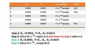
Name : Umma Hafsah Himu
Student ID : 1612524130
Topic : Concept of Bayesian
Approach
Group 4
Topic 10: Acceptance - rejection method
Name : Md. Emran Hossain
Roll : 1710824166
1
2
3
4
6
5
7
Name : Umma Hafsah Himu
Roll : 1612524130
Name : Al Helal Muhammad Swadhin
Roll : 1710624158
Name : Afsana Afruz Suchi
Roll : 1712524190
Name : Apu Chakraborty
Roll : 1711024180
Name : Saud Anwar Shawon
Roll : 1610424174
Name : Shohel Rana
Roll : 1710824135
• There are usually several alternative techniques that can be used for
generating random variates from a given distribution.
• Usually used when inverse transform is not directly applicable or is
inefficient (e.g., gamma, beta)
• The important techniques (methods) are:
1. Inverse transform technique
2. Composition technique
3. Convolution technique
4. Acceptance-rejection technique
Techniques for generating random variate
• In this technique, random variates with a distribution are
generated until some condition are satisfied.
• When the condition is finally satisfied, the desired random
variate can be computed.
Acceptance-Rejection technique
For example:
Suppose that an analyst needed to devise a method for
generating random variates, X, uniformly distributed
between ¼ and 1.
Step 1:
Generate a random number R.
Step 2a:
If R ≥ ¼, accept X=R, then go to step 3.
Step 2b:
If R < ¼, reject R, and return to step 1.
Step 3:
If another uniform random variate on [1/4, 1] is needed,
repeat the procedure beginning at step 1. If not stop.
One way to proceedwouldbe to followthese steps:
Step 2a is an “acceptance” and step 2b is a “rejection” in this
acceptance-rejection technique.
• A Poisson random variable, N, with mean α > 0 can be expressed as
• N can be interpreted as the number of arrivals from a Poisson arrival
process in one unit of time.
• But the interarrival times, A1, A2, … of successive customers are
exponentially distributed with rate α (i.e., α is the mean number of
arrivals per unit time).
Poisson distribution:
Example:
n = 0,1,…
• Thus there is a relationship between the (discrete) Poisson
distribution and the (continuous) exponential distribution,
namely:
N = n ---------------- (1)
• if and only if
---------------- (2)
• Clearly, these two statements are equivalent.
• Proceed now by generating exponential interarrival times until some
arrival, say n+1, occurs after time 1; then set N=n.
• Eqn. (1), N=n, says there were
exactly n arrivals during one unit
of time;
• but relation (2) says that the nth
arrival occurred before time 1 while
(n+1)st arrival occurred after time 1.
• For efficient generation purposes, relation (2) is usually simplified by
first using the exponential generating equation, 𝑨𝒊 = −
𝟏
α
𝐥𝐧 𝑹𝒊 , to
obtain
• Next multiply through by –α, which reverses the sign of the
inequality, and use the fact that a sum of logarithms is the logarithm
of a product, to get
• Finally, use the relation 𝒆𝒍𝒏 𝒙
= x for any number x to obtain
• which is equivalent to relation (2).
---------------- (3)
Step 1:
Set n=0, P=1
Step 2:
Generate a random number 𝑹 𝒏+𝟏 and replace P by P. 𝑹 𝒏+𝟏
Step 3:
If P < 𝒆−α, then accept N=n.
Otherwise, reject the current n, increase n by 1, and return to step 2.
The procedure for generating a Poisson random variate, N, is given
by the following steps:
Generate 3 Poisson variates with mean α=0.2. Use the following sequence
of random numbers, R: 0.4357, 0.4146, 0.8353, 0.9952, 0.8004, 0.7945.
Example: Poisson distribution:
Step 1: Set n=0, P=1
Step 2: 𝑹 𝟏=0.4357, P= 1. 𝑹 𝟏 =0.4357
Step 3: Since P=0.4357 < 𝒆−α = 𝒆− 𝟎.𝟐 =0.8187, accept N=0.
Step 1-3: (𝑹 𝟏=0.4146 leads to N=0)
Step 1: Set n=0, P=1
Step 2: 𝑹 𝟏=0.8353, P = 1. 𝑹 𝟏 =0.8353
Step 3: Since P≥ 𝒆−α, reject n=0 and return to step 2 with n=1
n R 𝐧+𝟏 P Accept/Reject Result
0 0.4357 0.4357 P < 𝐞−α (accept) N=0
0 0.4146 0.4146 P < 𝐞−α (accept) N=0
0 0.8353 0.8353 P ≥ 𝐞−α (reject)
1 0.9952 0.8313 P ≥ 𝐞−α (reject)
2 0.8004 0.6654 P < 𝐞−α (accept) N=2
Step 2: 𝑹 𝟐 =0.9952, P=𝑹 𝟏. 𝑹 𝟐=0.8313
Step 3: Since P≥ 𝒆−α, reject n=1 and return to step 2 with n=2
Step 2: 𝑹 𝟑=0.8004, P=𝑹 𝟏. 𝑹 𝟐. 𝑹 𝟑=0.6654
Step 3: Since P<𝒆−α , accept N=2.
References:
Slides and lectures of Professor Dr. Md. Rezaul Karim,
Department of Statistics, University of Rajshahi.
web.ics.purdue.edu/~hwan/IE680/Lectures/Chap08Slides
.pdf
Law, A. M., & W. Kelton (2000). Simulation modeling and
analysis. Mac Graw Hill, Boston, Burr Ridge, USA.
16

Generating random variates

  • 1.
    Name : UmmaHafsah Himu Student ID : 1612524130 Topic : Concept of Bayesian Approach Group 4 Topic 10: Acceptance - rejection method
  • 2.
    Name : Md.Emran Hossain Roll : 1710824166 1 2 3 4 6 5 7 Name : Umma Hafsah Himu Roll : 1612524130 Name : Al Helal Muhammad Swadhin Roll : 1710624158 Name : Afsana Afruz Suchi Roll : 1712524190 Name : Apu Chakraborty Roll : 1711024180 Name : Saud Anwar Shawon Roll : 1610424174 Name : Shohel Rana Roll : 1710824135
  • 3.
    • There areusually several alternative techniques that can be used for generating random variates from a given distribution. • Usually used when inverse transform is not directly applicable or is inefficient (e.g., gamma, beta) • The important techniques (methods) are: 1. Inverse transform technique 2. Composition technique 3. Convolution technique 4. Acceptance-rejection technique Techniques for generating random variate
  • 4.
    • In thistechnique, random variates with a distribution are generated until some condition are satisfied. • When the condition is finally satisfied, the desired random variate can be computed. Acceptance-Rejection technique
  • 5.
    For example: Suppose thatan analyst needed to devise a method for generating random variates, X, uniformly distributed between ¼ and 1.
  • 6.
    Step 1: Generate arandom number R. Step 2a: If R ≥ ¼, accept X=R, then go to step 3. Step 2b: If R < ¼, reject R, and return to step 1. Step 3: If another uniform random variate on [1/4, 1] is needed, repeat the procedure beginning at step 1. If not stop. One way to proceedwouldbe to followthese steps: Step 2a is an “acceptance” and step 2b is a “rejection” in this acceptance-rejection technique.
  • 7.
    • A Poissonrandom variable, N, with mean α > 0 can be expressed as • N can be interpreted as the number of arrivals from a Poisson arrival process in one unit of time. • But the interarrival times, A1, A2, … of successive customers are exponentially distributed with rate α (i.e., α is the mean number of arrivals per unit time). Poisson distribution: Example: n = 0,1,…
  • 8.
    • Thus thereis a relationship between the (discrete) Poisson distribution and the (continuous) exponential distribution, namely: N = n ---------------- (1) • if and only if ---------------- (2)
  • 9.
    • Clearly, thesetwo statements are equivalent. • Proceed now by generating exponential interarrival times until some arrival, say n+1, occurs after time 1; then set N=n. • Eqn. (1), N=n, says there were exactly n arrivals during one unit of time; • but relation (2) says that the nth arrival occurred before time 1 while (n+1)st arrival occurred after time 1.
  • 10.
    • For efficientgeneration purposes, relation (2) is usually simplified by first using the exponential generating equation, 𝑨𝒊 = − 𝟏 α 𝐥𝐧 𝑹𝒊 , to obtain • Next multiply through by –α, which reverses the sign of the inequality, and use the fact that a sum of logarithms is the logarithm of a product, to get
  • 11.
    • Finally, usethe relation 𝒆𝒍𝒏 𝒙 = x for any number x to obtain • which is equivalent to relation (2). ---------------- (3)
  • 12.
    Step 1: Set n=0,P=1 Step 2: Generate a random number 𝑹 𝒏+𝟏 and replace P by P. 𝑹 𝒏+𝟏 Step 3: If P < 𝒆−α, then accept N=n. Otherwise, reject the current n, increase n by 1, and return to step 2. The procedure for generating a Poisson random variate, N, is given by the following steps:
  • 13.
    Generate 3 Poissonvariates with mean α=0.2. Use the following sequence of random numbers, R: 0.4357, 0.4146, 0.8353, 0.9952, 0.8004, 0.7945. Example: Poisson distribution: Step 1: Set n=0, P=1 Step 2: 𝑹 𝟏=0.4357, P= 1. 𝑹 𝟏 =0.4357 Step 3: Since P=0.4357 < 𝒆−α = 𝒆− 𝟎.𝟐 =0.8187, accept N=0. Step 1-3: (𝑹 𝟏=0.4146 leads to N=0) Step 1: Set n=0, P=1 Step 2: 𝑹 𝟏=0.8353, P = 1. 𝑹 𝟏 =0.8353 Step 3: Since P≥ 𝒆−α, reject n=0 and return to step 2 with n=1
  • 14.
    n R 𝐧+𝟏P Accept/Reject Result 0 0.4357 0.4357 P < 𝐞−α (accept) N=0 0 0.4146 0.4146 P < 𝐞−α (accept) N=0 0 0.8353 0.8353 P ≥ 𝐞−α (reject) 1 0.9952 0.8313 P ≥ 𝐞−α (reject) 2 0.8004 0.6654 P < 𝐞−α (accept) N=2 Step 2: 𝑹 𝟐 =0.9952, P=𝑹 𝟏. 𝑹 𝟐=0.8313 Step 3: Since P≥ 𝒆−α, reject n=1 and return to step 2 with n=2 Step 2: 𝑹 𝟑=0.8004, P=𝑹 𝟏. 𝑹 𝟐. 𝑹 𝟑=0.6654 Step 3: Since P<𝒆−α , accept N=2.
  • 15.
    References: Slides and lecturesof Professor Dr. Md. Rezaul Karim, Department of Statistics, University of Rajshahi. web.ics.purdue.edu/~hwan/IE680/Lectures/Chap08Slides .pdf Law, A. M., & W. Kelton (2000). Simulation modeling and analysis. Mac Graw Hill, Boston, Burr Ridge, USA.
  • 16.