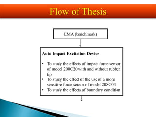
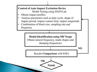
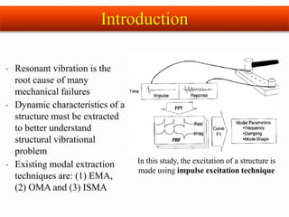
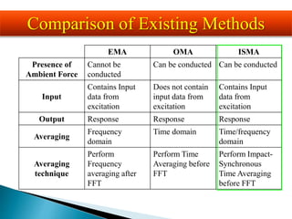
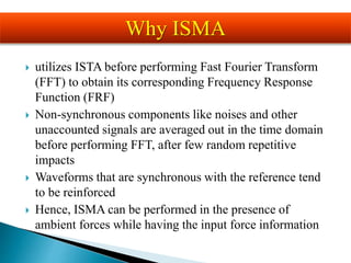
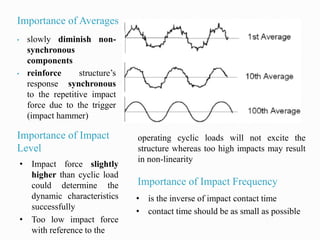
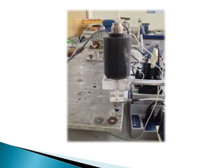
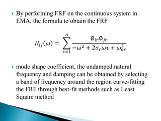
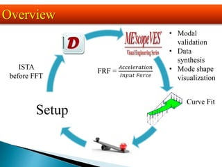
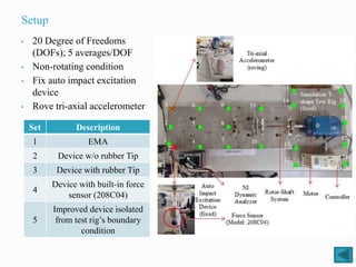
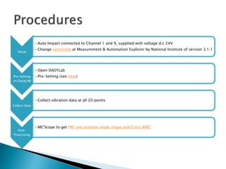
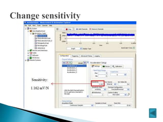
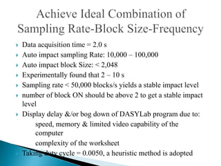
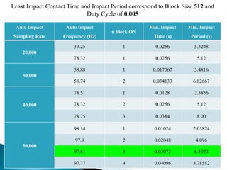
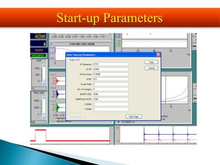
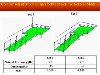
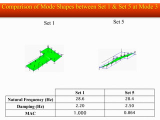
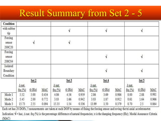
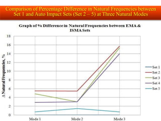
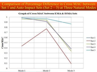
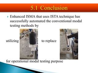
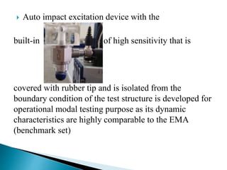
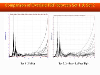
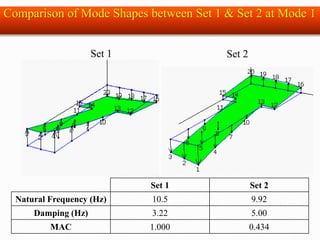
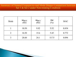
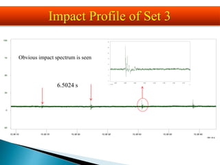
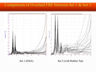
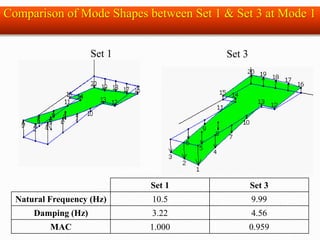
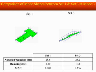
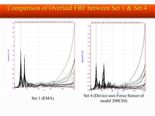
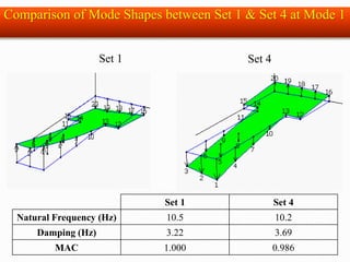
The document discusses the development and testing of an automated impact excitation device for modal analysis, focusing on the use of impulse excitation techniques to obtain dynamic characteristics of structures. It compares the effectiveness of Enhanced Impact Synchronous Modal Analysis (ISMA) against traditional Experimental Modal Analysis (EMA) under various conditions, emphasizing the automation's ability to deliver consistent impact levels and minimize labor. The study concludes that the automated device, particularly when equipped with a high-sensitivity force sensor and rubber tip, yields results comparable to benchmark EMA methods.

1. Lee Chia Chun (KEM100017)
session 2013/2014
Supervised by: Dr. Ong Zhi Chao
28-May 2014 (Wed)

2. EMA (benchmark)
Auto Impact Excitation Device
• To study the effects of impact force sensor
of model 200C20 with and without rubber
tip
• To study the effect of the use of a more
sensitive force sensor of model 208C04
• To study the effects of boundary condition
Flow of Thesis

3. Modal Identification using ME’Scope
Obtain natural frequency, mode shapes and
damping frequencies
Results Comparison with EMA
Finish
OK
NO
Control of Auto Impact Excitation Device
Modal Testing using DASYLab
• Obtain impact profiles
• Analyze parameters such as duty cycle, shape of
impact period, impact contact time, impact magnitude
• Combination of block size, sampling rate and
frequency

5. • Resonant vibration is the
root cause of many
mechanical failures
• Dynamic characteristics of a
structure must be extracted
to better understand
structural vibrational
problem
• Existing modal extraction
techniques are: (1) EMA,
(2) OMA and (3) ISMA
In this study, the excitation of a structure is
made using impulse excitation technique
Introduction

6. Current EMA Practice…
#experimental condition
#Labor-intensive
#Time-consuming
#Incur machine downtime cost
…Practice OMA Curren
#Lacks of input force informatio

7. EMA OMA ISMA
Presence of
Ambient Force
Cannot be
conducted
Can be conducted Can be conducted
Input
Contains Input
data from
excitation
Does not contain
input data from
excitation
Contains Input
data from
excitation
Output Response Response Response
Averaging
Frequency
domain
Time domain Time/frequency
domain
Averaging
technique
Perform
Frequency
averaging after
FFT
Perform Time
Averaging before
FFT
Perform Impact-
Synchronous
Time Averaging
before FFT
Comparison of Existing Methods

8.  utilizes ISTA before performing Fast Fourier Transform
(FFT) to obtain its corresponding Frequency Response
Function (FRF)
 Non-synchronous components like noises and other
unaccounted signals are averaged out in the time domain
before performing FFT, after few random repetitive
impacts
 Waveforms that are synchronous with the reference tend
to be reinforced
 Hence, ISMA can be performed in the presence of
ambient forces while having the input force information
Why ISMA

9. Importance of Averages
• slowly diminish non-
synchronous
components
• reinforce structure’s
response synchronous
to the repetitive impact
force due to the trigger
(impact hammer)
• Impact force slightly
higher than cyclic load
could determine the
dynamic characteristics
successfully
• Too low impact force
with reference to the
operating cyclic loads will not excite the
structure whereas too high impacts may result
in non-linearity
Importance of Impact
Level
Importance of Impact Frequency
• is the inverse of impact contact time
• contact time should be as small as possible

10.  has difficulty in extracting dynamic characteristics of a
structure which is closer to the operating speed for high speed
machines
 perform badly if the impact frequency in ISMA is synchronous
with the running speed
 performs random impacts using manually operated impact
hammer which is labour-intensive and time-consuming
 Manual procedures result in inconsistency in terms of impact
contact time, impact period and impact level, as well as human
errors e.g. double impact
 This gives rise to the need of automating ISMA
Limitation of ISMA

12.  To control and synchronize the portable
calibrated auto impact excitation device with
virtual instruments
 To study the impact profiles generated by
the auto impact excitation device which
facilitates ISMA
 To compare and verify the dynamic
characteristics obtained by auto impact
excitation device to that obtained by EMA
during non-rotating condition (benchmark)
Objectives

14.  Obtain modal parameters under experimental
conditions
 Conducted in complete shutdown mode
 Excitation force applied in the time domain, but the
system responses are auto-correlated with the
measured input (Peter Avitabile, 2001; Peres & Bono,
2011)
 The correlated functions are transformed into
frequency domain to obtain the transfer functions
(FRF)
2.1 Experimental Modal Analysis (EMA)

15.  𝑋 𝜔 = 𝐻 𝜔 ∙ 𝑄 𝜔 where 𝑋 𝜔 and 𝑄 𝜔 are
n x 1 frequency vectors of accelerations and forces
respectively. 𝐻 𝜔 is an n x n square matrix of FRF
of the system. It also regarded as accelerance
(Hosseini, Arzanpour, Golnaraghi, & Parameswaran,
2013)

16. Alternatively, can be written as,
𝑋𝑖 = 𝑗=1
𝑛
𝐻𝑖𝑗 ∙ 𝑄𝑗
 (Chao, 2013), in page 30, describes above constitutes
a reciprocal theorem for dynamic loads that is
similar to Maxwell’s reciprocal theorem for static
loads
 So, it is OK to rove or fix any of the impact hammer
or the force transducer

17.  By performing FRF on the continuous system in
EMA, the formula to obtain the FRF
𝐻𝑖𝑗 𝜔 =
𝑟=1
𝑛
∅𝑖𝑟∅ 𝑗𝑟
−𝜔2 + 2𝜎𝑟 𝜔𝒾 + 𝜔 𝑜𝑟
2
 mode shape coefficient, the undamped natural
frequency and damping can be obtained by selecting
a band of frequency around the region curve-fitting
the FRF through best-fit methods such as Least
Square method

18.  Linear superimposition of unaccounted responses
with response due to trigger
 𝑋 𝜔 = 𝐻1 𝜔 ∙ 𝐹1 + 𝐻2 𝜔 ∙ 𝐹2 + 𝐻3 𝜔 ∙ 𝐹3 + ⋯
2.2 Conducting EMA during Operation

19. Time
Enhanced
Time
Enhanced
Spectrum
Auto-
spectrum
Input
Trigger
Averaging Analysis Squaring
**Requires trigger signal to be synchronous with
the periodic signal of interest
(A G A Rahman, 2013)
Auto-spectrum, 𝐺 𝑋𝑋 = 𝐺 𝐴𝐴 + 1 𝑁 ×
𝐺 𝑀𝑀
deterministic component, 𝐺 𝐴𝐴
noise/unaccounted component, 𝐺 𝑀𝑀
Importance of average number
𝑦 𝑡 =
1
𝑁
𝑟=0
𝑁−1
𝑥(𝑡 + 𝑟𝑇𝑂)
2.3 Impact-Synchronous Time Domain
Averaging Method

20.  create an impact through virtual instrument, at a
shortest possible impact contact time that would
automatically on and off periodically at constant and
shortest possible impact period and constant impact
level
s
0 .00 0 .25 0 .50 0 .75 1 .00 1 .25 1 .50 1 .75
Y /tCha rt0
5 .0
2 .5
0 .0
-2 .5
-5 .0
2.4 Control of Auto Impact Excitation Device

21.  time response block is defined as the block size, BS over the
sampling rate, SR:
tblock =
BS
SR
 The period of square wave, T is defined as the inverse of
frequency, f of the square wave:
T =
1
f
 The number of cycle of square wave within the response time
block is:
n =
tblock
T
(n = integers; otherwise, truncate decimals)
 Duty cycle is the percentage of one period in which a signal is
active and is given by:
tON = DC × T
The square wave signals can only moves along the time axis
provided that there is a time difference, ∆t. Hence, the condition of
∆t ≠ 0 ∴𝑡 𝑏𝑙𝑜𝑐𝑘 ≠ nT, must be met. Hence, is given by:
∆t = tblock − nT

22.  Next, the number of block which is On, N can be evaluated as:
N =
tON
∆t
(N = integers; otherwise, truncate decimals)
 The impact contact time, 𝑇𝑝𝑢𝑙𝑠𝑒 is evaluated by taking the number
of blocks which is On, to multiply by the time response
block,𝑡 𝑏𝑙𝑜𝑐𝑘:
Tpulse =
tON
∆t
× tblock = N × tblock
 The impact period is determined by using:
Tinterval =
𝑇
∆t
× tblock
 The inverse of Tinterval gives the impact frequency:
fimpact =
1
Tinterval
a heuristic method is adopted to determine a range of accepted
combination of sampling rate-block size-frequency-duty cycle

23.  quantitative technique to compare the closeness between two
families of mode shapes x(1) and x(2) (Allemang, 2003;
Allemang & Brown, 1998; Peter Avitabile, 2001)
 MAC (𝑥(𝑖)
(1)
, 𝑥(𝑗)
(2)
) =
𝑥(𝑖)
(1)
𝑥(𝑗)
(2)
𝑥(𝑖)
(1)
𝑥(𝑗)
(2)
2
 indicates whether there are enough measurement points for the
modal analysis (Gaetan Kerschen, 2006)
MAC Value Interpretation
= 1.0 Two mode shapes are identical
> 0.9 Two mode shapes are similar
< 0.9 Two mode shapes are different
2.5 Modal Assurance Criteria (MAC)

25. Goals:
 To acquire impact profiles of the test structure
obtained by using the auto impact excitation to
compare with EMA
 To obtain the dynamic characteristics of the test
structure to compare and validated with EMA
3.1 Methodology

26. Setup
FRF =
𝐴𝑐𝑐𝑒𝑙𝑒𝑟𝑎𝑡𝑖𝑜𝑛
𝐼𝑛𝑝𝑢𝑡 𝐹𝑜𝑟𝑐𝑒
Curve Fit
ISTA
before FFT
Overview
• Modal
validation
• Data
synthesis
• Mode shape
visualization

27. Setup
• 20 Degree of Freedoms
(DOFs); 5 averages/DOF
• Non-rotating condition
• Fix auto impact excitation
device
• Rove tri-axial accelerometer
Set Description
1 EMA
2 Device w/o rubber Tip
3 Device with rubber Tip
4
Device with built-in force
sensor (208C04)
5
Improved device isolated
from test rig’s boundary
condition

28. Setup
•Auto Impact connected to Channel 1 and 9, supplied with voltage d.c 24V
•Change sensitivity at Measurement & Automation Explorer by National Institute of version 3.1.1
Pre-Setting
on DasyLAB
•Open DASYLab
•Pre-Setting (see here)
Collect Data
•Collect vibration data at all 20 points
Post-
Processing
•ME’Scope to get FRF and animate mode shape and Cross MAC

30. Pre-Setting Interface

33. Too low/high
Trigger level
Cabling
Avoid double
impact
Set a pre-
trigger delay

36.  To control and synchronize the portable
calibrated auto impact excitation device with
virtual instruments
 To study the impact profiles generated by
the auto impact excitation device which
facilitates ISMA
 To compare and verify the dynamic
characteristics obtained by auto impact
excitation device to that obtained by EMA
during non-rotating condition (benchmark)
Objectives

37. m s
0 .0 2 .5 5 .0 7 .5 10 .0 12 .5 15 .0 17 .5 20 .0
Y /tChart0
5 .0
2 .5
0 .0
-2 .5
-5 .0
Duty Cycle of 0.0050 (0.5%)

38. h :m in :s
12 :39 :30 12 :39 :40 12 :39 :50 12 :40 :00 12 :40 :10 12 :40 :20
50
45
40
35
30
25
20
15
10
5
0
-5
R eco rde r0
6.5024 s35N

39. Set 1 (EMA) Set 5
h :m in :s
13 :23 :10 .520 13 :23 :10 .530 13 :23 :10 .540 13 :23 :10 .550
60
50
40
30
20
10
0
-10
R eco rde r0
h:m in:s
12:40:07.250 12:40:07.255 12:40:07.260 12:40:07.265 12:40:07.270
50
45
40
35
30
25
20
15
10
5
0
-5
Recorder0
0.00342 s 0.00586 s
Duty Cycle of 0.0050 (0.5%)

40.  Data acquisition time = 2.0 s
 Auto impact sampling Rate: 10,000 – 100,000
 Auto impact block Size: < 2,048
 Experimentally found that 2 – 10 s
 Sampling rate < 50,000 blocks/s yields a stable impact level
 number of block ON should be above 2 to get a stable impact
level
 Display delay &/or bog down of DASYLab program due to:
speed, memory & limited video capability of the
computer
complexity of the worksheet
 Taking duty cycle = 0.0050, a heuristic method is adopted

41. Auto Impact
Sampling Rate
Auto Impact
Frequency (Hz)
n block ON
Min. Impact
Time (s)
Min. Impact
Period (s)
20,000
39.25 1 0.0256 5.3248
78.32 1 0.0256 5.12
30,000
58.88 1 0.017067 3.4816
58.74 2 0.034133 6.82667
40,000
78.51 1 0.0128 2.5856
78.32 2 0.0256 5.12
78.25 3 0.0384 8.00
50,000
98.14 1 0.01024 2.05824
97.9 2 0.02048 4.096
97.81 3 0.03072 6.5024
97.77 4 0.04096 8.78582
Least Impact Contact Time and Impact Period correspond to Block Size 512 and
Duty Cycle of 0.005

42. Start-up Parameters

44.  To control and synchronize the portable
calibrated auto impact excitation device with
virtual instruments
 To study the impact profiles generated by
the auto impact excitation device which
facilitates ISMA
 To compare and verify the dynamic
characteristics obtained by auto impact
excitation device to that obtained by EMA
during non-rotating condition (benchmark)
Objectives

45. Qualitative comparison:
• Overlaid Frequency Response Function (FRF) Spectral
• Mode Shape
Quantitative comparison:
• Difference in Natural Frequencies
• Modal Assurance Criteria (MAC)

46. Comparison between Set 1 & Set 5

47. Set 1 (EMA)
Set 5 (Device Isolated from the
Boundary Condition of the Test Rig)
Comparison of Overlaid FRF between Set 1 &Set 5

48. Set 1 Set 5
Set 1 Set 5
Natural Frequency (Hz) 10.5 10.5
Damping (Hz) 3.22 2.88
MAC 1.000 0.981
Comparison of Mode Shapes between Set 1 & Set 5 at Mode 1

49. Set 1 Set 5
Set 1 Set 5
Natural Frequency (Hz) 16.5 16.4
Damping (Hz) 1.45 1.64
MAC 1.000 0.966
Comparison of Mode Shapes between Set 1 & Set 5 at Mode 2

50. Set 1 Set 5
Set 1 Set 5
Natural Frequency (Hz) 28.6 28.4
Damping (Hz) 2.20 2.50
MAC 1.000 0.864
Comparison of Mode Shapes between Set 1 & Set 5 at Mode 3

51. Mode
𝝎 𝐒𝐞𝐭 𝟏
(Hz)
𝝎 𝐒𝐞𝐭 𝟓
(Hz)
∆𝝎
(%)
MAC
1 10.50 10.50 0.00 0.981
2 16.50 16.40 0.61 0.966
3 28.60 28.40 0.70 0.864
Summary of Natural Frequencies and Mode Shapes Comparison between
Set 1 & Set 5 under Non-rotating Condition

52. Result Summary from Set 2 - 5

53. Comparison of Percentage Difference in Natural Frequencies between
Set 1 and Auto Impact Sets (Set 2 – 5) at Three Natural Modes

54. Comparison of Percentage Difference in Cross MAC between
Set 1 and Auto Impact Sets (Set 2 – 5) at Three Natural Modes

56.  Enhanced ISMA that uses ISTA technique has
successfully automated the conventional modal
testing methods by
utilizing to replace
for operational modal testing purpose
5.1 Conclusion

57.  The enhanced ISMA can automatically deliver impact
onto a structure at a consistent impact level over
constant impact period, at a very small impact contact
time to accurately and effortlessly acquire the
dynamic characteristics of a test structure under non-
rotating condition
 The impact profile can be changed by the auto impact
sampling rate, block size, frequency and duty cycle
readily with the use of auto impact excitation device

58.  Auto impact excitation device with the
built-in of high sensitivity that is
covered with rubber tip and is isolated from the
boundary condition of the test structure is developed for
operational modal testing purpose as its dynamic
characteristics are highly comparable to the EMA
(benchmark set)

59.  Perform the enhanced ISMA technique on a rotating
structure for verification purpose
 Create a programming algorithm in the virtual
instrument (DASYLab) to immediately stop the data
acquisition process after the running components and
noises are successfully filtered out
 Devise a practical way to isolate the auto impact
excitation device from the boundary condition of a
test structure
5.2 Recommendation

60. Questions?

62. Comparison between Different Values of Duty
Cycle

63. m s
0 .0 2 .5 5 .0 7 .5 10 .0 12 .5 15 .0 17 .5 20 .0 22 .5 25 .0 27 .5 30 .0 32 .5 35 .0 37 .5 40 .0
Y /tChart0
5 .0
2 .5
0 .0
-2 .5
-5 .0
Impact Profile when Duty Cycle = 0.50

64. Impact Response Zoomed Impact Response
h :m in :s
12 :39 :35 12 :39 :45 12 :39 :55 12 :40 :05 12 :40 :15 12 :40 :25 12 :40 :35
60
50
40
30
20
10
0
-10
R eco rde r0 h :m in :s
12 :40 :09 .70 12 :40 :09 .85 12 :40 :10 .00 12 :40 :10 .15 12 :40 :10 .30 12 :40 :10 .45 12 :40 :10 .60
60
50
40
30
20
10
0
-10
R eco rde r0

65. m s
0 .0 2 .5 5 .0 7 .5 10 .0 15 .0 20 .0 25 .0 30 .0 35 .0 40 .0
Y /tChart0
5 .0
2 .5
0 .0
-2 .5
-5 .0
Impact Profile when Duty Cycle = 0.01

66. Impact Response Zoomed Impact Response
h :m in :s
12 :39 :25 12 :39 :35 12 :39 :45 12 :39 :55 12 :40 :05 12 :40 :15 12 :40 :25
60
50
40
30
20
10
0
-10
R eco rde r0 h :m in :s
12 :39 :59 .0 12 :39 :59 .5 12 :40 :00 .0 12 :40 :00 .5 12 :40 :01 .0
60
50
40
30
20
10
0
-10
R eco rde r0

67. Comparison between Set 1 & Set 2

68. h :m in :s
1 :46 :45 11 :46 :50 11 :46 :55 11 :47 :00 11 :47 :05 11 :47 :10 11 :47 :15 11 :47 :20 11 :47 :25 11 :47 :30 11 :47 :35 11 :47 :40 11 :47 :45
100
75
50
25
0
-25
Recorder0
h :m in :s
11 :46 :59 .85 11 :46 :59 .90 11 :46 :59 .95 11 :47 :00 .00 11 :47 :00 .05 11 :47 :00 .10 11 :47 :00 .15 11 :47 :00 .20 11 :47 :00 .25
100
75
50
25
0
-25
Reco rde r0
6.5024 s
Impact Profile of Set 2
Presence of double impact

69. Set 1 (EMA) Set 2 (without Rubber Tip)
Comparison of Overlaid FRF between Set 1 & Set 2

70. Set 1 Set 2
Set 1 Set 2
Natural Frequency (Hz) 10.5 9.92
Damping (Hz) 3.22 5.00
MAC 1.000 0.434
Comparison of Mode Shapes between Set 1 & Set 2 at Mode 1

71. Set 1 Set 2
Set 1 Set 2
Natural Frequency (Hz) 16.5 15.6
Damping (Hz) 1.45 2.00
MAC 1.000 0.772
Comparison of Mode Shapes between Set 1 & Set 2 at Mode 2

72. Set 1 Set 2
Set 1 Set 2
Natural Frequency (Hz) 28.6 24.1
Damping (Hz) 2.20 2.55
MAC 1.000 0.094
Comparison of Mode Shapes between Set 1 & Set 2 at Mode 3

73. Mode
𝝎 𝐒𝐞𝐭 𝟏
(Hz)
𝝎 𝐒𝐞𝐭 2
(Hz)
∆𝝎
(%)
MAC
1 10.50 9.92 5.52 0.434
2 16.50 15.6 5.45 0.772
3 28.60 24.1 15.73 0.094
Summary of Natural Frequencies and Mode Shapes Comparison between
Set 1 & Set 2 under Non-rotating Condition

74. Comparison between Set 1 & Set 3

75. Impact Profile of Set 3
h :m in :s
12 :05 :10 12 :05 :15 12 :05 :20 12 :05 :25 12 :05 :30 12 :05 :35 12 :05 :40
100
75
50
25
0
-25
s
30 .00 30 .25 30 .50 30 .75 31 .00 31 .25 31 .50 31 .75
Y /tChart0
30
25
20
15
10
5
0
-5
6.5024 s
Obvious impact spectrum is seen

76. Set 1 (EMA) Set 3 (with Rubber Tip)
Comparison of Overlaid FRF between Set 1 & Set 3

77. Set 1 Set 3
Set 1 Set 3
Natural Frequency (Hz) 10.5 9.99
Damping (Hz) 3.22 4.56
MAC 1.000 0.959
Comparison of Mode Shapes between Set 1 & Set 3 at Mode 1

78. Set 1 Set 3
Set 1 Set 3
Natural Frequency (Hz) 16.5 16.0
Damping (Hz) 1.45 1.66
MAC 1.000 0.942
Comparison of Mode Shapes between Set 1 & Set 3 at Mode 2

79. Set 1 Set 3
Set 1 Set 3
Natural Frequency (Hz) 28.6 24.2
Damping (Hz) 2.20 1.54
MAC 1.000 0.336
Comparison of Mode Shapes between Set 1 & Set 3 at Mode 3

80. Mode
𝝎 𝐒𝐞𝐭 𝟏
(Hz)
𝝎 𝐒𝐞𝐭 3
(Hz)
∆𝝎
(%)
MAC
1 10.50 9.99 4.86 0.959
2 16.50 16.00 3.03 0.942
3 28.60 24.20 15.35 0.336
Summary of Natural Frequencies and Mode Shapes Comparison between
Set 1 & Set 3 under Non-rotating Condition

81. Comparison between Set 1 & Set 4

82. Set 1 (EMA)
Set 4 (Device uses Force Sensor of
model 208C04)
Comparison of Overlaid FRF between Set 1 & Set 4

83. Set 1 Set 4
Set 1 Set 4
Natural Frequency (Hz) 10.5 10.2
Damping (Hz) 3.22 3.69
MAC 1.000 0.986
Comparison of Mode Shapes between Set 1 & Set 4 at Mode 1

84. Set 1 Set 4
Set 1 Set 4
Natural Frequency (Hz) 16.5 16.0
Damping (Hz) 1.45 1.87
MAC 1.000 0.912
Comparison of Mode Shapes between Set 1 & Set 4 at Mode 2

85. Set 1 Set 4
Set 1 Set 4
Natural Frequency (Hz) 28.6 24.6
Damping (Hz) 2.20 1.50
MAC 1.000 0.379
Comparison of Mode Shapes between Set 1 & Set 4 at Mode 3

86. Mode
𝝎 𝐒𝐞𝐭 𝟏
(Hz)
𝝎 𝐒𝐞𝐭 4
(Hz)
∆𝝎
(%)
MAC
1 10.50 10.20 2.86 0.986
2 16.50 16.00 3.03 0.912
3 28.60 24.60 13.99 0.379
Summary of Natural Frequencies and Mode Shapes Comparison between
Set 1 & Set 4 under Non-rotating Condition

87. Gantt Chart (Sem 1)

88. Gantt Chart (Sem 2)