Download to read offline

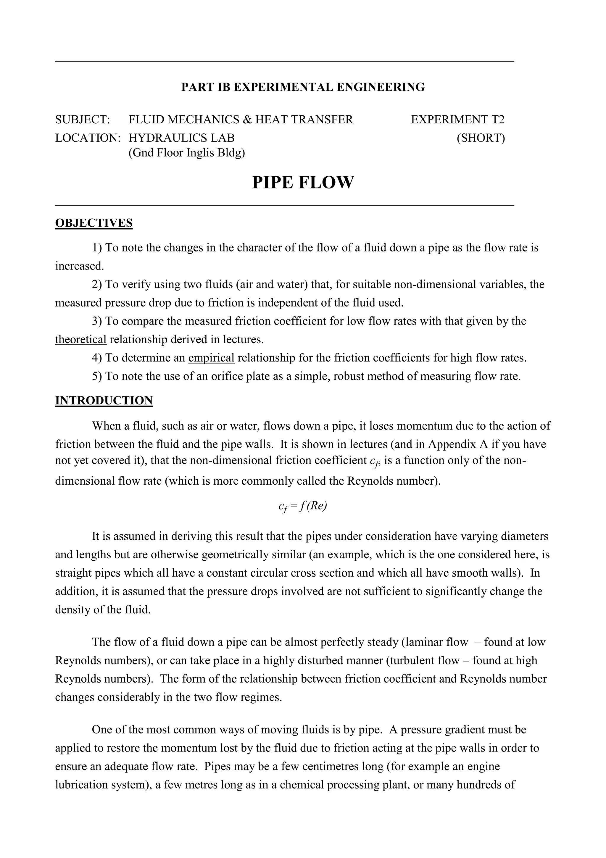
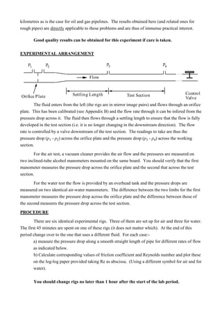
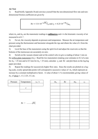

1) This document describes an experiment on fluid mechanics involving the flow of air and water through pipes. 2) The objectives are to study how friction changes with flow rate, verify that friction is independent of fluid type, compare measurements to theory, and determine an empirical relationship for high flow rates. 3) The procedure involves measuring pressure drops across an orifice plate and test section for increasing flow rates, and plotting the results on log-log scales to analyze friction coefficients versus Reynolds numbers.