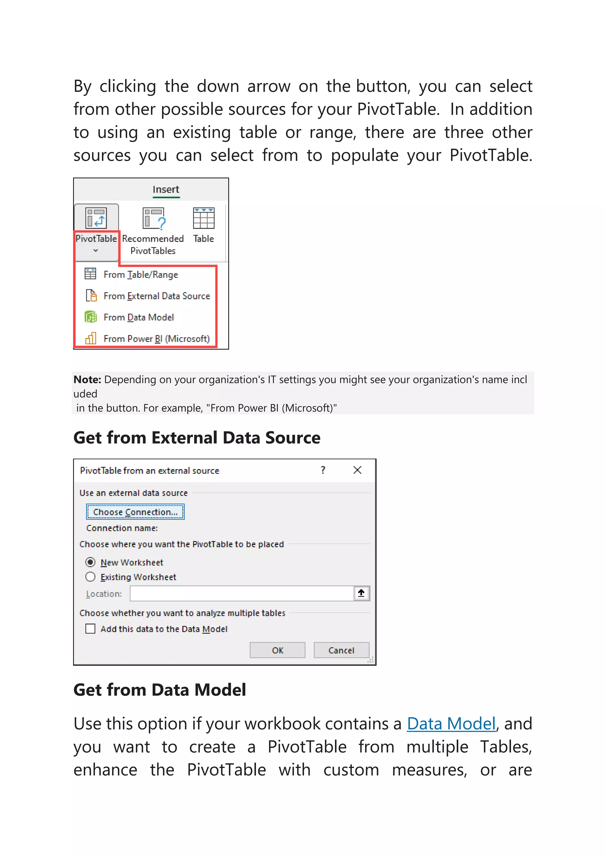
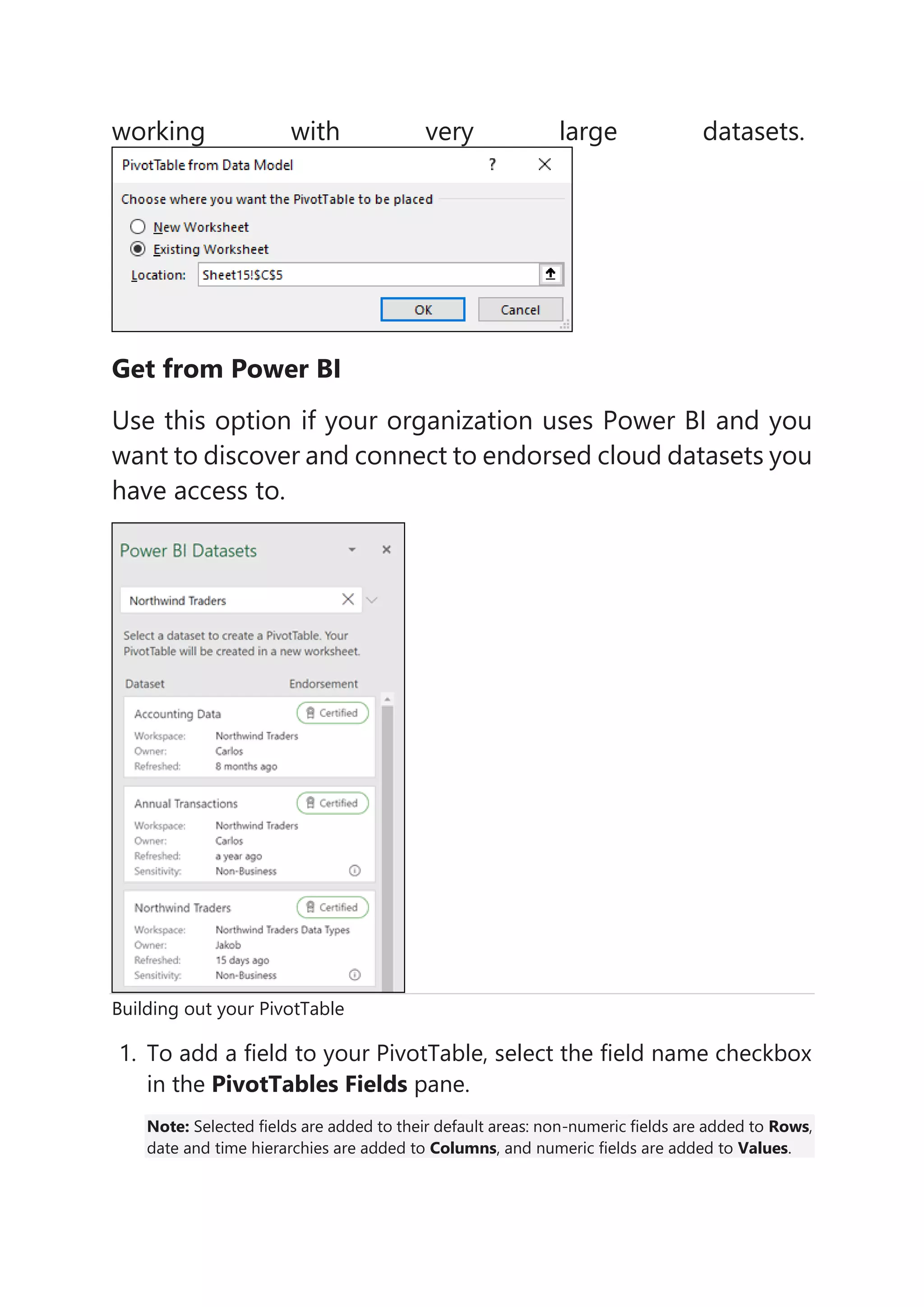
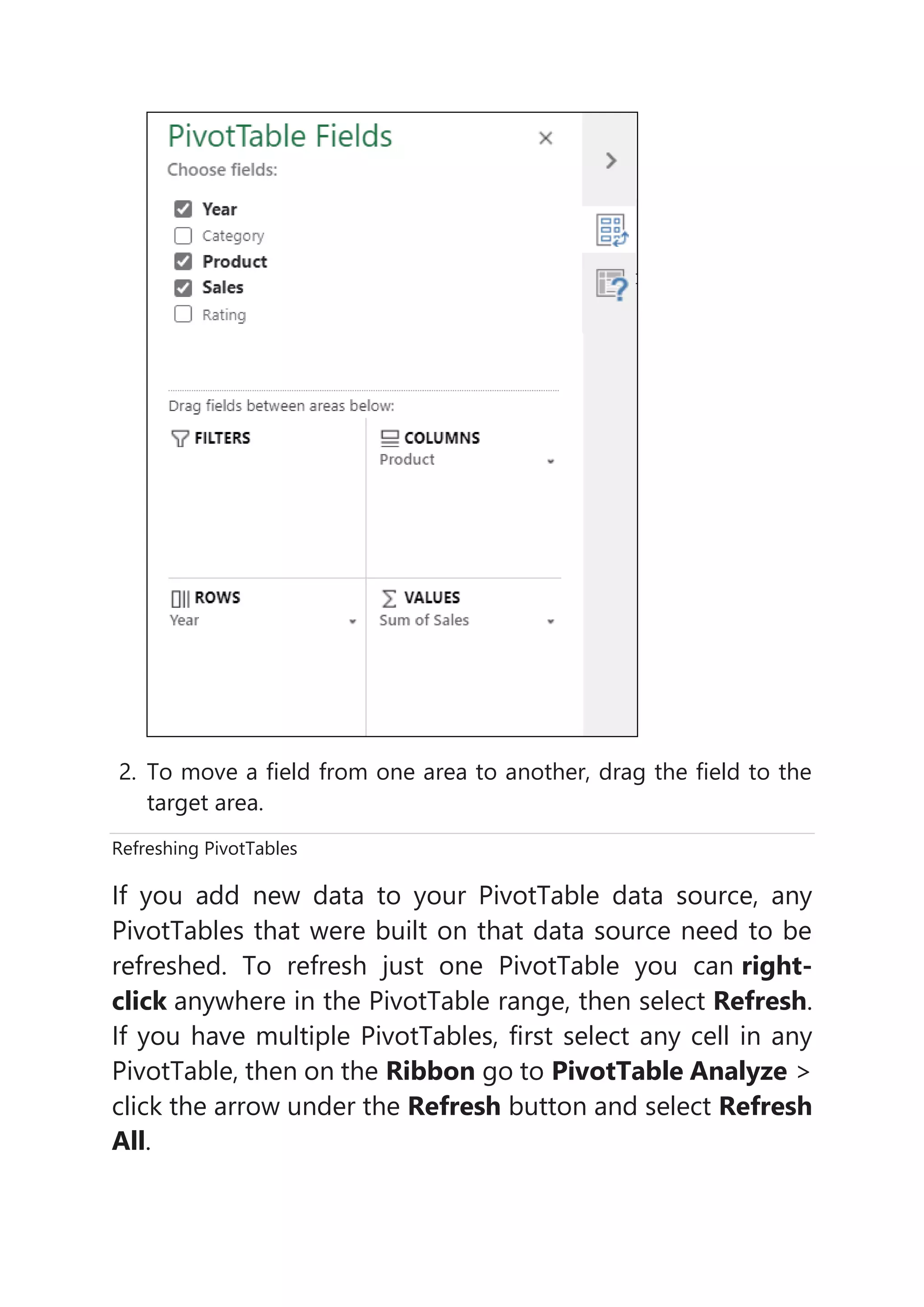
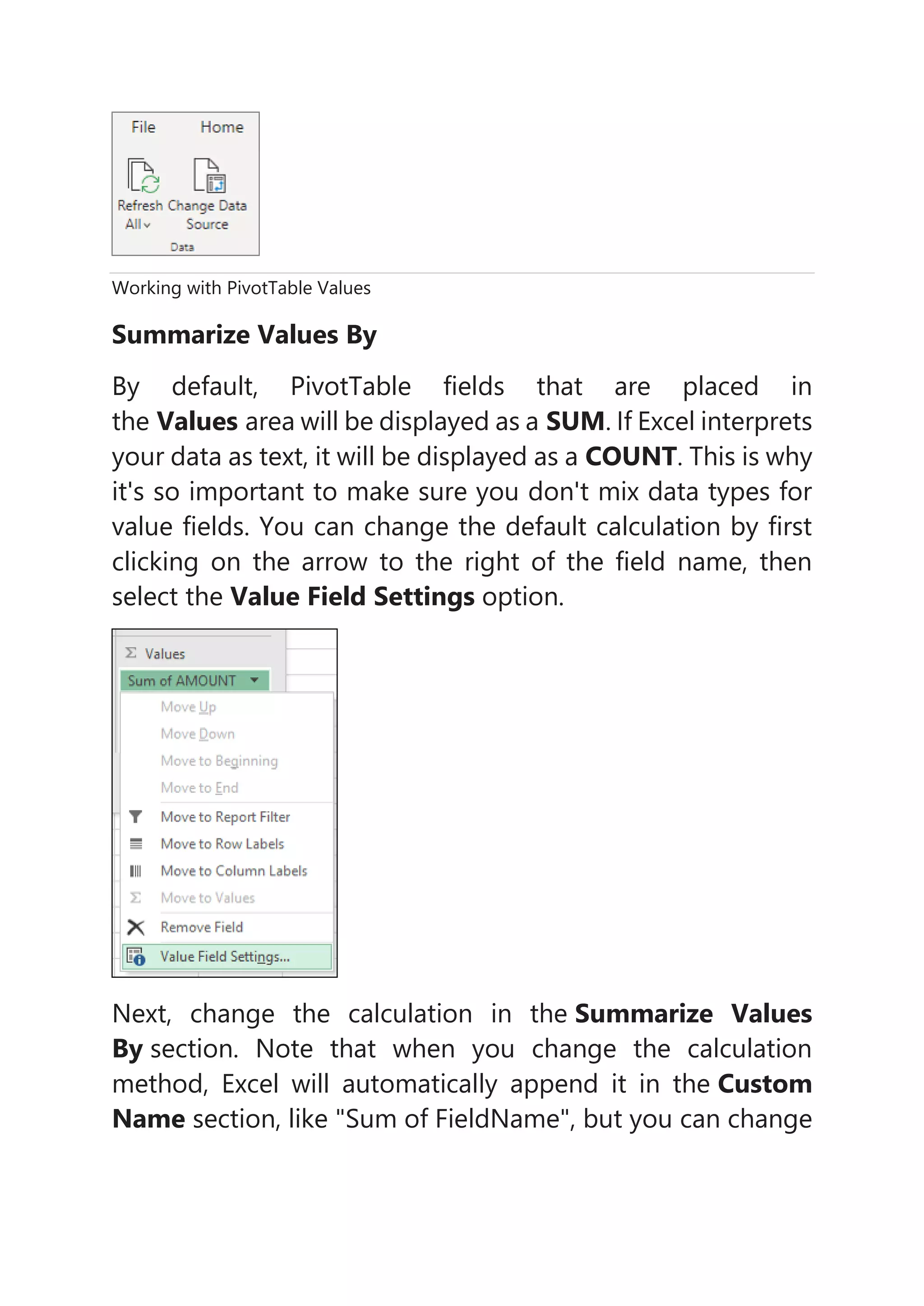
1) A PivotTable is a tool in Excel that allows users to analyze and summarize data by automatically calculating comparisons in the data. 2) PivotTables can retrieve data from an existing table or range, an external data source, a data model, or Power BI depending on the options selected by the user. 3) Users can build out a PivotTable by adding fields to the rows, columns, and values areas and then refresh the PivotTable if the underlying data is updated.

1. Create a PivotTable
to analyze
worksheet data
Excel for Microsoft 365 Excel for Microsoft 365 for Mac Excel for
the web More...
You on hurry! Watch this video
A PivotTable is a powerful tool to calculate, summarize,
and analyze data that lets you see comparisons,
patterns, and trends in your data. PivotTables work a
little bit differently depending on what platform you
are using to run Excel.
WindowsWebMac
Create a PivotTable in Excel for Windows
PivotTables from other sources

2. By clicking the down arrow on the button, you can select
from other possible sources for your PivotTable. In addition
to using an existing table or range, there are three other
sources you can select from to populate your PivotTable.
Note: Depending on your organization's IT settings you might see your organization's name incl
uded
in the button. For example, "From Power BI (Microsoft)"
Get from External Data Source
Get from Data Model
Use this option if your workbook contains a Data Model, and
you want to create a PivotTable from multiple Tables,
enhance the PivotTable with custom measures, or are

3. working with very large datasets.
Get from Power BI
Use this option if your organization uses Power BI and you
want to discover and connect to endorsed cloud datasets you
have access to.
Building out your PivotTable
1. To add a field to your PivotTable, select the field name checkbox
in the PivotTables Fields pane.
Note: Selected fields are added to their default areas: non-numeric fields are added to Rows,
date and time hierarchies are added to Columns, and numeric fields are added to Values.

4. 2. To move a field from one area to another, drag the field to the
target area.
Refreshing PivotTables
If you add new data to your PivotTable data source, any
PivotTables that were built on that data source need to be
refreshed. To refresh just one PivotTable you can right-
click anywhere in the PivotTable range, then select Refresh.
If you have multiple PivotTables, first select any cell in any
PivotTable, then on the Ribbon go to PivotTable Analyze >
click the arrow under the Refresh button and select Refresh
All.

5. Working with PivotTable Values
Summarize Values By
By default, PivotTable fields that are placed in
the Values area will be displayed as a SUM. If Excel interprets
your data as text, it will be displayed as a COUNT. This is why
it's so important to make sure you don't mix data types for
value fields. You can change the default calculation by first
clicking on the arrow to the right of the field name, then
select the Value Field Settings option.
Next, change the calculation in the Summarize Values
By section. Note that when you change the calculation
method, Excel will automatically append it in the Custom
Name section, like "Sum of FieldName", but you can change

6. it. If you click the Number Format button, you can change
the number format for the entire field.
Tip: Since the changing the calculation in the Summarize Values By section will change the
PivotTable field name, it's best not to rename your PivotTable fields until you're done setting up
your PivotTable. One trick is to use Find & Replace (Ctrl+H) >Find what > "Sum of",
then Replace with > leave blank to replace everything at once instead of manually retyping.
Show Values As
Instead of using a calculation to summarize the data, you can
also display it as a percentage of a field. In the following
example, we changed our household expense amounts to
display as a % of Grand Total instead of the sum of the
values.

7. Once you've opened the Value Field Setting dialog, you can
make your selections from the Show Values As tab.
Display a value as both a calculation and percentage.
Simply drag the item into the Values section twice, then set
the Summarize Values By and Show Values As options for
each one.