This document is an instructor's manual designed to accompany the fifth edition of 'Elementary Linear Algebra' by Stephen Andrilli and David Hecker. It includes answers to exercises and chapter tests for all chapters in the textbook, along with detailed solutions for most problems. The manual serves as a resource for instructors to facilitate teaching and assessment in linear algebra courses.


![Answers to Exercises Section 1.1
Answers to Exercises
Chapter 1
Section 1.1
(1) (a) [9 −4], distance =
√
97
(b) [−6 1 1], distance =
√
38
(c) [−1 −1 2 −3 −4], distance =
√
31
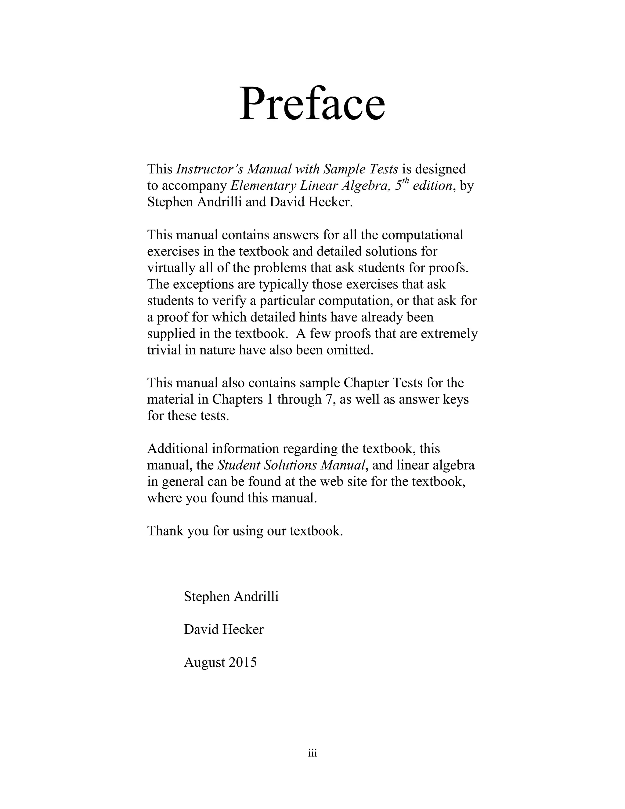
(2) (a) (3 4 2) (see Figure 1)
(b) (0 5 3) (see Figure 2)
(c) (1 −2 0) (see Figure 3)
(d) (3 0 0) (see Figure 4)
(3) (a) (7 −13) (b) (6 4 −8) (c) (−1 3 −1 4 6)
(4) (a)
¡16
3 −13
3 8
¢
(b) (−20
3 −1 −6 −1)
(5) (a)
h
3√
70
− 5√
70
6√
70
i
; shorter, since length of original vector is 1
(b)
£
−6
7 2
7 0 −3
7
¤
; shorter, since length of original vector is 1
(c) [06 −08]; neither, since given vector is a unit vector
(d)
h
1√
11
− 2√
11
− 1√
11
1√
11
2√
11
i
; longer, since length of original vector =
√
11
5 1
(6) (a) Parallel (b) Parallel (c) Not parallel (d) Not parallel
(7) (a) [−6 12 15]
(b) [10 6 −12]
(c) [−7 1 11]
(d) [−9 −2 4]
(e) [−10 −32 −1]
(f) [−35 3 20]
(8) (a) x + y = [1 1], x − y = [−3 9], y − x = [3 −9] (see Figure 5)
(b) x + y = [3 −5], x − y = [17 1], y − x = [−17 −1] (see Figure 6)
(c) x + y = [1 8 −5], x − y = [3 2 −1], y − x = [−3 −2 1] (see Figure 7)
(d) x + y = [−2 −4 4], x − y = [4 0 6], y − x = [−4 0 −6] (see Figure 8)
(9) With = (7 −3 6), = (11 −5 3), and = (10 −7 8), the length of side = length of side
=
√
29. The triangle is isosceles, but not equilateral, since the length of side is
√
30.
(10) (a) [10 −10] (b) [−5
√
3 −15] (c) [0 0] = 0
(11) See Figures 1.7 and 1.8 in Section 1.1 of the textbook.
Copyright c° 2016 Elsevier Ltd. All rights reserved. 1](https://image.slidesharecdn.com/elementary-linear-algebra-5th-edition-larson-solutions-manual-190402053218/75/Elementary-Linear-Algebra-5th-Edition-Larson-Solutions-Manual-5-2048.jpg)

![Answers to Exercises Section 1.1
(12) See Figure 9. Both represent the same diagonal vector by the associative law of addition for vectors.
Figure 9: x + (y + z)
(13) [05 − 06
√
2 −04
√
2] ≈ [−03485 −05657]
(14) Net velocity = [−2
√
2 −3 + 2
√
2], resultant speed ≈ 283 km/hr
(15) Net velocity =
h
−3
√
2
2 8−3
√
2
2
i
; speed ≈ 283 km/hr
(16) [−8 −
√
2 −
√
2]
(17) Acceleration = 1
20 [12
13 −344
65 392
65 ] ≈ [00462 −02646 03015]
(18) Acceleration =
£13
2 0 4
3
¤
(19) 180√
14
[−2 3 1] ≈ [−9622 14432 4811]
(20) a = [ −
1+
√
3
1+
√
3
]; b = [
1+
√
3
√
3
1+
√
3
]
(21) Let a = [1 ].
(a) kak2
= 2
1 + · · · + 2
is a sum of squares, which must be nonnegative. But then ||a|| ≥ 0 because
the square root of a nonnegative real number is a nonnegative real number.
(b) If ||a|| = 0, then kak2
= 2
1 + · · · + 2
= 0, which is only possible if every = 0. Thus, a = 0.
(22) In each part, suppose that x = [1 ], y = [1 ], and z = [1 ].
(a) x + (y + z) = [1 ] + [(1 + 1) ( + )] = [(1 + (1 + 1)) ( + ( + ))]
= [((1 + 1) + 1) (( + ) + )] = [(1 + 1) ( + )] + [1 ] = (x + y) + z
(b) x + (−x) = [1 ] + [−1 −] = [(1 + (−1)) ( + (−))] = [0 0]. Also,
(−x) + x = x + (−x) (by part (1) of Theorem 1.3) = 0, by the above.
(c) (x+y) = ([(1+1) (+)]) = [(1+1) (+)] = [(1+1) (+)] =
[1 ] + [1 ] = x + y
Copyright c° 2016 Elsevier Ltd. All rights reserved. 4](https://image.slidesharecdn.com/elementary-linear-algebra-5th-edition-larson-solutions-manual-190402053218/75/Elementary-Linear-Algebra-5th-Edition-Larson-Solutions-Manual-8-2048.jpg)
![Answers to Exercises Section 1.2
(d) ()x = [(()1) (())] = [((1)) (())] = [(1) ()]
= ([1 ]) = (x)
(23) If = 0, done. Otherwise, (1
)(x) = 1
(0) =⇒ (1
· )x = 0 (by part (7) of Theorem 1.3) =⇒ x = 0
Thus either = 0 or x = 0.
(24) 1x = 2x =⇒ 1x − 2x = 0 =⇒ (1 − 2)x = 0 =⇒ (1 − 2) = 0 or x = 0 by Theorem 1.4. But
since 1 6= 2 (1 − 2) 6= 0 Hence, x = 0
(25) (a) F (b) T (c) T (d) F (e) T (f) F (g) F (h) F
Section 1.2
(1) (a) arccos(− 27
5
√
37
), or about 1526◦
, or 266 radians
(b) arccos( 46√
74
√
29
), or about 68◦
, or 012 radians
(c) arccos(0), which is 90◦
, or
2 radians
(d) arccos(− 435√
2175
√
87
) = arccos(−1), which is 180◦
, or radians (since x = −5y)
(2) The vector from 1 to 2 is [2 −7 −3], and the vector from 1 to 3 is [5 4 −6]. These vectors are
orthogonal.
(3) (a) [ ] · [− ] = (−) + = 0 Similarly, [ −] · [ ] = 0
(b) A vector in the direction of the line + + = 0 is [ −], while a vector in the direction of
− + = 0 is [ ].
(4) (a) 15 joules (b) 1040
√
5
9 ≈ 2584 joules (c) −189
√
15
5 ≈ −1464 joules
(5) Note that y·z is a scalar, so x·(y·z) is not defined.
(6) In all parts, let x = [1 2 ] y = [1 2 ] and z = [1 2 ]
(a) x · y = [1 2 ] · [1 2 ] = 11 + · · · + = 11 + · · · +
= [1 2 ] · [1 2 ] = y · x
(b) x · x = [1 2 ] · [1 2 ] = 11 + · · · + = 2
1 + · · · + 2
. Now 2
1 + · · · + 2
is a sum of squares, each of which must be nonnegative. Hence, the sum is also nonnegative, and
so its square root is defined. Thus, 0 ≤ x · x = 2
1 + · · · + 2
=
³p
2
1 + · · · + 2
´2
= kxk2
.
(c) Suppose x · x = 0. From part (b), 0 = x · x = 2
1 + · · · + 2
≥ 2
, for each , since all terms in the
sum are nonnegative. Hence, 0 ≥ 2
for each . But 2
≥ 0, because it is a square. Hence each
= 0. Therefore, x = 0.
(d) (x · y) = ([1 2 ] · [1 2 ]) = (11 + · · · + )
= 11 + · · · + = [1 2 ] · [1 2 ] = (x) · y.
Next, (x · y) = (y · x) (by part (a)) = (y) · x (from above) = x · (y), by part (a)
Copyright c° 2016 Elsevier Ltd. All rights reserved. 5](https://image.slidesharecdn.com/elementary-linear-algebra-5th-edition-larson-solutions-manual-190402053218/75/Elementary-Linear-Algebra-5th-Edition-Larson-Solutions-Manual-9-2048.jpg)
![Answers to Exercises Section 1.2
(e) (x + y) · z = ([1 2 ] + [1 2 ]) · [1 2 ]
= [1 + 1 2 + 2 + ] · [1 2 ]
= (1 + 1)1 + (2 + 2)2 + · · · + ( + )
= (11 + 22 + · · · + ) + (11 + 22 + · · · + )
Also, (x · z) + (y · z) = ([1 2 ] · [1 2 ]) + ([1 2 ] · [1 2 ])
= (11 + 22 + · · · + ) + (11 + 22 + · · · + ).
Hence, (x + y) · z = (x · z) + (y · z).
(7) No; consider x = [1 0], y = [0 1], and z = [1 1].
(8) A method similar to the first part of the proof of Lemma 1.6 in the textbook yields:
ka − bk
2
≥ 0 =⇒ (a · a) − (b · a) − (a · b) + (b · b) ≥ 0 =⇒ 1 − 2(a · b) + 1 ≥ 0 =⇒ a · b ≤ 1.
(9) Note that (x + y)·(x − y) = (x·x) + (y·x) − (x·y) − (y·y) = kxk2
− kyk2
. Hence, (x + y)·(x − y) = 0
implies kxk2
= kyk2
, which means kxk = kyk (since both are nonnegative)
(10) Note that kx + yk2
= kxk2
+ 2(x·y) + kyk2
, while kx − yk2
= kxk2
− 2(x·y) + kyk2
.
Hence, 1
2 (kx + yk2
+ kx − yk2
) = 1
2 (2kxk2
+ 2kyk2
) = kxk2
+ kyk2
(11) (a) From the first equation in the solution to Exercise 10 above, kx + yk2
= kxk2
+ kyk2
implies
2(x·y) = 0 which means x·y = 0.
(b) From the first equation in the solution to Exercise 10 above, x·y = 0 implies kx+yk2
= kxk2
+kyk2
.
(12) Note that kx + y + zk2
= k(x + y) + zk2
= kx + yk2
+ 2((x + y)·z) + kzk2
= kxk2
+ 2(x·y) + kyk2
+ 2(x·z) + 2(y·z) + kzk2
= kxk2
+ kyk2
+ kzk2
since x, y, z are mutually orthogonal.
(13) From the first two equations in the solution for Exercise 10 above,
1
4 (kx + yk2
− kx − yk2
) = 1
4 (4(x·y)) = x·y.
(14) Since x is orthogonal to both y and z, we have x·(1y + 2z) = 1(x·y) + 2(x·z) = 1(0) + 2(0) = 0
(15) Suppose y = x, for some 6= 0 Then, x · y = x·(x) = (x · x) = kxk2
= kxk ( kxk) = kxk (±|| kxk)
= ± kxk kxk = ± kxk kyk
(16) (a) Length =
√
3 (b) angle = arccos(
√
3
3 ) ≈ 547◦
, or 0955 radians
(17) (a) projab = [−3
5 − 3
10 −3
2 ]; b − projab = [8
5 43
10 −3
2 ]; (b − projab) · a = 0
(b) projab = [−6
5 1 2
5 ]; b − projab = [−14
5 −4 8
5 ]; (b − projab) · a = 0
(c) projab = [1
6 0 −1
6 1
3 ]; b − projab = [17
6 −1 1
6 −4
3 ]; (b − projab) · a = 0
(d) projab = [−1 3
2 −2 −3
2 ]; b − projab = [6 −1
2 −6 7
2 ]; (b − projab) · a = 0
(18) (a) 0 (zero vector). The dropped perpendicular travels along b to the common initial point of a and
b.
(b) The vector b. The terminal point of b lies on the line through a, so the dropped perpendicular
has length zero.
Copyright c° 2016 Elsevier Ltd. All rights reserved. 6](https://image.slidesharecdn.com/elementary-linear-algebra-5th-edition-larson-solutions-manual-190402053218/75/Elementary-Linear-Algebra-5th-Edition-Larson-Solutions-Manual-10-2048.jpg)
![Answers to Exercises Section 1.2
(19) i, j, k
(20) (a) Parallel: [20
29 −30
29 40
29 ], orthogonal: [−194
29 88
29 163
29 ]
(b) Parallel: [−1
2 1 − 1
2 ], orthogonal: [−11
2 1 15
2 ]
(c) Parallel: [60
49 −40
49 120
49 ], orthogonal: [−354
49 138
49 223
49 ]
(21) From the lower triangle in the figure, we have (projrx) + (projrx − x) = reflection of x (see Figure
10).
Figure 10: Reflection of a vector x through a line.
(22) For the case kxk ≤ kyk: | kxk − kyk | = kyk − kxk = kx + y + (−x)k − kxk ≤ kx + yk + k − xk − kxk
(by the Triangle Inequality) = kx + yk + kxk − kxk = kx + yk.
The case kxk ≥ kyk is done similarly, with the roles of x and y reversed.
(23) (a) Note that projxy = [8
5 −6
5 2] = 2
5 x and y − projxy = [7
5 −24
5 −4] is orthogonal to x.
Let w = y − projxy Then since y = projxy + (y − projxy) we have y = 2
5 x + w where w is
orthogonal to x.
(b) Let = (x·y)(kxk2
) (so that x = projxy), and let w = y − projxy which is orthogonal to x
by the argument before Theorem 1.11. Then y = x + w, where w is orthogonal to x.
(c) Suppose x+w = x+v. Then (−)x = w−v, and (−)x·(w−v) = (w−v)·(w−v) = kw−vk2
.
But (−)x·(w −v) = (−)(x·w)−(−)(x·v) = 0, since v and w are orthogonal to x. Hence
kw − vk2
= 0 =⇒ w − v = 0 =⇒ w = v. Then, x = x =⇒ = , from Theorem 1.4, since x is
nonzero.
(24) If is the angle between x and y, and is the angle between projxy and projyx, then
cos =
projxy · projyx
kprojxyk
°
°projyx
°
° =
³
x·y
kxk2
´
x ·
³
y·x
kyk2
´
y
°
°
°
³
x·y
kxk2
´
x
°
°
°
°
°
°
³
y·x
kyk2
´
y
°
°
°
=
³
x·y
kxk2
´ ³
y·x
kyk2
´
(x · y)
³
|x·y|
kxk2
´
kxk
³
|y·x|
kyk2
´
kyk
=
³
(x·y)3
kxk2
kyk2
´
³
(x·y)2
kxkkyk
´ =
(x · y)
kxk kyk
= cos
Hence = .
Copyright c° 2016 Elsevier Ltd. All rights reserved. 7](https://image.slidesharecdn.com/elementary-linear-algebra-5th-edition-larson-solutions-manual-190402053218/75/Elementary-Linear-Algebra-5th-Edition-Larson-Solutions-Manual-11-2048.jpg)
![Answers to Exercises Section 1.3
(25) (a) T (b) T (c) F (d) F (e) T (f) F
Section 1.3
(1) (a) We have k4x + 7yk ≤ k4xk + k7yk = 4kxk + 7kyk ≤ 7kxk + 7kyk = 7(kxk + kyk).
(b) Let = max{|| ||}. Then kx ± yk ≤ (kxk + kyk).
(2) (a) Note that 6 − 5 = 3(2( − 1)) + 1. Let = 2( − 1).
(b) Consider the number 4.
(3) Note that since x 6= 0 and y 6= 0, projxy = 0 iff (x·y)(kxk2
) = 0 iff x·y = 0 iff y·x = 0 iff
(y·x)(kyk2
) = 0 iff projyx = 0.
(4) If y = x (for 0), then kx + yk = kx + xk = (1 + )kxk = kxk + kxk = kxk + kxk = kxk + kyk.
On the other hand, if kx + yk = kxk + kyk, then kx + yk2
= (kxk + kyk)2
. Now kx + yk2
=
(x + y)·(x + y) = kxk2
+ 2(x·y) + kyk2
, while (kxk + kyk)2
= kxk2
+ 2kxkkyk + kyk2
. Hence
x·y = kxkkyk. By Result 4, y = x, for some 0.
(5) (a) Suppose y 6= 0. We must show that x is not orthogonal to y. Now kx + yk2
= kxk2
, so
kxk2
+ 2(x·y) + kyk2
= kxk2
. Hence kyk2
= −2(x·y). Since y 6= 0, we have kyk2
6= 0, and so
x·y 6= 0.
(b) Suppose x is not a unit vector. We must show that x·y 6= 1.
Now projxy = x =⇒ ((x·y)(kxk2
))x = 1x =⇒ (x·y)(kxk2
) = 1 =⇒ x·y = kxk2
.
But then kxk 6= 1 =⇒ kxk2
6= 1 =⇒ x·y 6= 1.
(6) (a) Consider x = [1 0 0] and y = [1 1 0].
(b) If x 6= y, then x · y 6= kxk2
.
(c) Yes
(7) See the answer for Exercise 11(a) in Section 1.2.
(8) If kxk kyk, then kxk2
kyk2
, and so kxk2
− kyk2
0 But then (x + y)·(x−y) 0 and so the
cosine of the angle between (x + y) and (x−y) is positive. Thus the angle between (x + y) and (x−y)
is acute.
(9) (a) Contrapositive: If x = 0, then x is not a unit vector.
Converse: If x is nonzero, then x is a unit vector.
Inverse: If x is not a unit vector, then x = 0.
(b) (Let x and y be nonzero vectors.)
Contrapositive: If y 6= projxy, then x is not parallel to y.
Converse: If y = projxy, then x k y.
Inverse: If x is not parallel to y, then y 6= projxy.
(c) (Let x, y be nonzero vectors.)
Contrapositive: If projyx 6= 0, then projxy 6= 0.
Converse: If projyx = 0, then projxy = 0.
Inverse: If projxy 6= 0, then projyx 6= 0.
(10) (a) Converse: Let x and y be nonzero vectors in R
. If kx + yk kyk, then x·y ≥ 0.
Copyright c° 2016 Elsevier Ltd. All rights reserved. 8](https://image.slidesharecdn.com/elementary-linear-algebra-5th-edition-larson-solutions-manual-190402053218/75/Elementary-Linear-Algebra-5th-Edition-Larson-Solutions-Manual-12-2048.jpg)
![Answers to Exercises Section 1.3
(b) Let x = [2 −1] and y = [0 2].
(11) (a) Converse: Let x, y, and z be vectors in R
. If y = z, then x·y = x·z. The converse is obviously
true, but the original statement is false in general, with counterexample x = [1 1], y = [1 −1],
and z = [−1 1].
(b) Converse: Let x and y be vectors in R
. If kx + yk ≥ kyk, then x · y = 0. The original
statement is true, but the converse is false in general. Proof of the original statement follows from
kx + yk2
= (x + y) · (x + y) = kxk2
+ 2(x · y) + kyk2
= kxk2
+ kyk2
≥ kyk2
.
Counterexample to converse: let x = [1 0], y = [1 1].
(c) Converse: Let x, y be vectors in R
, with 1. If x = 0 or y = 0, then x·y = 0. The converse
is obviously true, but the original statement is false in general, with counterexample x = [1 −1]
and y = [1 1].
(12) Suppose x ⊥ y and is odd. Then x · y = 0. Now x · y =
P
=1 . But each product equals
either 1 or −1. If exactly of these products equal 1, then x · y = − ( − ) = − + 2. Hence
− + 2 = 0, and so = 2, contradicting odd.
(13) Suppose that [6 5], [−2 3], and [1 2] are mutually orthogonal, with [1 2] 6= [0 0]. Then 61+52 =
0 and −21 + 32 = 0. Multiplying the latter equation by 3, we obtain −61 + 92 = 0 Adding this
to the first equation gives 142 = 0, which means 2 = 0, and hence 1 = 0. Thus, [1 2] = [0 0], a
contradiction.
(14) Assume that ||x|| = 1. We know that ||projxy|| 6= x·y However, projxy =
¡
(x·y)||x||2
¢
x so
||projxy|| = |x·y|||x||2
= |x·y| But x · y 0 because the angle between x and y is acute, so
||projxy|| = x·y, a contradiction. Thus, ||x|| 6= 1
(15) Base Step ( = 1): x1 = x1.
Inductive Step: Assume x1 + x2 + · · · + x−1 + x = x + x−1 + · · · + x2 + x1, for some ≥ 1
Prove: x1 + x2 + · · · + x−1 + x + x+1 = x+1+ x + x−1 + · · · + x2 + x1
But,
x1 + x2 + · · · + x−1 + x + x+1 = (x1 + x2 + · · · + x−1 + x) + x+1
= x+1 + (x1 + x2 + · · · + x−1 + x)
= x+1 + (x + x−1 + · · · + x2 + x1)
(by the inductive hypothesis)
= x+1 + x + x−1 + · · · + x2 + x1
(16) Base Step ( = 1): kx1k ≤ kx1k.
Inductive Step: Assume kx1 + · · · + xk ≤ kx1k + · · · + kxk, for some ≥ 1.
Prove: kx1 + · · · + x + x+1k ≤ kx1k + · · · + kxk + kx+1k.
But, by the Triangle Inequality,
k(x1 + · · · + x) + x+1k ≤ kx1 + · · · + xk + kx+1k
≤ kx1k + · · · + kxk + kx+1k
by the inductive hypothesis.
(17) Base Step ( = 1): kx1k2
= kx1k2
.
Inductive Step: Assume kx1 + · · · + xk2
= kx1k2
+ · · · + kxk2
.
Copyright c° 2016 Elsevier Ltd. All rights reserved. 9](https://image.slidesharecdn.com/elementary-linear-algebra-5th-edition-larson-solutions-manual-190402053218/75/Elementary-Linear-Algebra-5th-Edition-Larson-Solutions-Manual-13-2048.jpg)
![Answers to Exercises Section 1.3
Prove: kx1 + · · · + x + x+1k2
= kx1k2
+ · · · + kxk2
+ kx+1k2
.
We have
k(x1 + · · · + x) + x+1k2
= kx1 + · · · + xk2
+ 2((x1 + · · · + x)·x+1) + kx+1k2
= kx1 + · · · + xk2
+ kx+1k2
(since x+1is orthogonal to all of x1 x)
= kx1k2
+ · · · + kxk2
+ kx+1k2
by the inductive hypothesis.
(18) Base Step ( = 1): We must show (1x1)·y ≤ |1| kyk.
But,
(1x1)·y ≤ |(1x1)·y| ≤ k1x1k kyk
(by the Cauchy-Schwarz Inequality)
= |1| kx1k kyk = |1| kyk
since x1 is a unit vector.
Inductive Step: Assume (1x1 + · · · + x)·y ≤ (|1| + · · · + ||)kyk, for some ≥ 1.
Prove: (1x1 + · · · + x + +1x+1)·y ≤ (|1| + · · · + || + |+1|)kyk.
We have
((1x1 + · · · + x) + +1x+1)·y = (1x1 + · · · + x)·y + (+1x+1)·y
≤ (|1| + · · · + ||)kyk + (+1x+1)·y
(by the inductive hypothesis)
≤ (|1| + · · · + ||)kyk + |+1| ||y||
(by an argument similar to the Base Step)
= (|1| + · · · + || + |+1|)kyk
(19) Step 1 cannot be reversed, because could equal ±(2
+ 2).
Step 2 cannot be reversed, because 2
could equal 4
+ 42
+ .
Step 4 cannot be reversed, because in general does not have to equal 2
+ 2.
Step 6 cannot be reversed, since
could equal 2 + .
All other steps remain true when reversed.
(20) (a) For every unit vector x in R3
, x · [1 −2 3] 6= 0.
(b) x 6= 0 and x·y ≤ 0, for some vectors x and y in R
.
(c) x = 0 or kx + yk 6= kyk, for all vectors x and y in R
.
(d) There is some vector x ∈ R
for which x·x ≤ 0.
(e) There is an x ∈ R3
such that for every nonzero y ∈ R3
, x · y 6= 0.
(f) For every x ∈ R4
, there is some y ∈ R4
such that x·y 6= 0.
(21) (a) Contrapositive: If x 6= 0 and kx − yk ≤ kyk, then x · y 6= 0.
Converse: If x = 0 or kx − yk kyk, then x · y = 0.
Inverse: If x · y 6= 0, then x 6= 0 and kx − yk ≤ kyk.
Copyright c° 2016 Elsevier Ltd. All rights reserved. 10](https://image.slidesharecdn.com/elementary-linear-algebra-5th-edition-larson-solutions-manual-190402053218/75/Elementary-Linear-Algebra-5th-Edition-Larson-Solutions-Manual-14-2048.jpg)
![Answers to Exercises Section 1.4
(b) Contrapositive: If kx − yk ≤ kyk, then either x = 0 or x·y 6= 0.
Converse: If kx − yk kyk, then x 6= 0 and x·y = 0.
Inverse: If x = 0 or x·y 6= 0, then kx − yk ≤ kyk.
(22) Suppose x 6= 0. We must prove x·y 6= 0 for some vector y ∈ R
. Let y = x.
(23) Let x = [1 1], y = [1 −1].
(24) Let y = [1 −2 2]. Then since x·y ≥ 0, Result 3 implies that kx + yk kyk = 3.
(25) (a) F (b) T (c) T (d) F (e) F (f) F (g) F (h) T (i) F
Section 1.4
(1) (a)
⎡
⎣
2 1 3
2 7 −5
9 0 −1
⎤
⎦
(b) Impossible
(c)
⎡
⎣
−16 8 12
0 20 −4
24 4 −8
⎤
⎦
(d)
⎡
⎣
−32 8 6
−8 2 14
0 6 −8
⎤
⎦
(e) Impossible
(f)
⎡
⎣
−7 0 8
−1 3 1
9 9 −5
⎤
⎦
(g)
⎡
⎣
−23 14 −9
−5 8 8
−9 −18 1
⎤
⎦
(h) Impossible
(i)
⎡
⎣
−1 1 12
−1 5 8
8 −3 −4
⎤
⎦
(j)
⎡
⎣
−1 1 12
−1 5 8
8 −3 −4
⎤
⎦
(k)
∙
−12 8 −6
10 −8 26
¸
(l) Impossible
(m) Impossible
(n)
⎡
⎣
13 −6 2
3 −3 −5
3 5 1
⎤
⎦
(2) Square: B C E F G H J K L M N P Q
Diagonal: B G N
Upper triangular: B G L N
Lower triangular: B G M N Q
Symmetric: B F G J N P
Skew-symmetric: H (but not E C K)
Transposes: A
=
∙
−1 0 6
4 1 0
¸
, B
= B, C
=
∙
−1 −1
1 1
¸
, and so on
(3) (a)
⎡
⎢
⎢
⎣
3 −1
2
5
2
− 1
2 2 1
5
2 1 2
⎤
⎥
⎥
⎦ +
⎡
⎢
⎢
⎣
0 −1
2
3
2
1
2 0 4
− 3
2 −4 0
⎤
⎥
⎥
⎦
(b)
⎡
⎢
⎢
⎣
1 3
2 0
3
2 3 −1
0 −1 0
⎤
⎥
⎥
⎦ +
⎡
⎢
⎢
⎣
0 −3
2 −4
3
2 0 0
4 0 0
⎤
⎥
⎥
⎦
(c)
⎡
⎢
⎢
⎣
2 0 0 0
0 5 0 0
0 0 −2 0
0 0 0 5
⎤
⎥
⎥
⎦ +
⎡
⎢
⎢
⎣
0 3 4 −1
−3 0 −1 2
−4 1 0 0
1 −2 0 0
⎤
⎥
⎥
⎦
Copyright c° 2016 Elsevier Ltd. All rights reserved. 11](https://image.slidesharecdn.com/elementary-linear-algebra-5th-edition-larson-solutions-manual-190402053218/75/Elementary-Linear-Algebra-5th-Edition-Larson-Solutions-Manual-15-2048.jpg)
![Answers to Exercises Section 1.5
(13) (a) Trace (B) = 1, trace (C) = 0, trace (E) = −6, trace (F) = 2, trace (G) = 18, trace (H) = 0,
trace (J) = 1, trace (K) = 4, trace (L) = 3, trace (M) = 0, trace (N) = 3, trace (P) = 0,
trace (Q) = 1
(b) Part (i): Let D = A+B. Then trace(D) =
P
=1 =
P
=1 +
P
=1 = trace(A)+trace(B).
Part (ii): Let B = A. Then trace(B) =
P
=1 =
P
=1 =
P
=1 = (trace(A)).
Part (iii): Let B = A
. Then trace(B) =
P
=1 =
P
=1 (since = for all ) = trace(A).
(c) Not necessarily: consider the matrices L and N in Exercise 2. (Note: If = 1, the statement is
true.)
(14) (a) F (b) T (c) F (d) T (e) T
Section 1.5
(1) (a) Impossible
(b)
⎡
⎣
34 −24
42 49
8 −22
⎤
⎦
(c) Impossible
(d)
⎡
⎣
73 −34
77 −25
19 −14
⎤
⎦
(e) [−38]
(f)
⎡
⎣
−24 48 −16
3 −6 2
−12 24 −8
⎤
⎦
(g) Impossible
(h) [56 −8]
(i) Impossible
(j) Impossible
(k)
⎡
⎣
22 9 −6
9 73 18
2 −6 4
⎤
⎦
(l)
⎡
⎢
⎢
⎣
5 3 2 5
4 1 3 1
1 1 0 2
4 1 3 1
⎤
⎥
⎥
⎦
(m) [226981]
(n)
⎡
⎣
146 5 −603
154 27 −560
38 −9 −193
⎤
⎦
(o) Impossible
(2) (a) No (b) Yes (c) No (d) Yes (e) No
(3) (a) [15 −13 −8]
(b)
⎡
⎣
11
6
3
⎤
⎦
(c) [4]
(d) [2 8 −2 12]
(4) (a) Valid, by Theorem 1.16, part (1)
(b) Invalid
(c) Valid, by Theorem 1.16, part (1)
(d) Valid, by Theorem 1.16, part (2)
(e) Valid, by Theorem 1.18
(f) Invalid
(g) Valid, by Theorem 1.16, part (3)
(h) Valid, by Theorem 1.16, part (2)
(i) Invalid
(j) Valid, by Theorem 1.16, part (3),
and Theorem 1.18
(5)
Outlet 1
Outlet 2
Outlet 3
Outlet 4
Salary Fringe Benefits
⎡
⎢
⎢
⎣
$367500 $78000
$225000 $48000
$765000 $162000
$360000 $76500
⎤
⎥
⎥
⎦
Copyright c° 2016 Elsevier Ltd. All rights reserved. 13](https://image.slidesharecdn.com/elementary-linear-algebra-5th-edition-larson-solutions-manual-190402053218/75/Elementary-Linear-Algebra-5th-Edition-Larson-Solutions-Manual-17-2048.jpg)
![Answers to Exercises Section 1.5
(6)
June
July
August
Tickets Food Souvenirs
⎡
⎣
$1151300 $3056900 $2194400
$1300700 $3456700 $2482400
$981100 $2615900 $1905100
⎤
⎦
(7)
Nitrogen
Phosphate
Potash
Field 1 Field 2 Field 3
⎡
⎣
100 045 065
090 035 075
095 035 085
⎤
⎦(in tons)
(8)
Rocket 1
Rocket 2
Rocket 3
Rocket 4
Chip 1 Chip 2 Chip 3 Chip 4
⎡
⎢
⎢
⎣
2131 1569 1839 2750
2122 1559 1811 2694
2842 2102 2428 3618
2456 1821 2097 3124
⎤
⎥
⎥
⎦
(9) (a) One example:
∙
1 1
0 −1
¸
(b) One example:
⎡
⎣
1 1 0
0 −1 0
0 0 1
⎤
⎦
(c) Consider
⎡
⎣
0 0 1
1 0 0
0 1 0
⎤
⎦
(10) (a) Third row, fourth column entry of AB
(b) Fourth row, first column entry of AB
(c) Third row, second column entry of BA
(d) Second row, fifth column entry of BA
(11) (a)
P
=1 32 (b)
P
=1 41
(12) (a) [−27 43 −56]
(b)
⎡
⎣
56
−57
18
⎤
⎦
(13) (a) [−61 15 20 9]
(b)
⎡
⎣
43
−41
−12
⎤
⎦
(14) (a) Let B = Ai. Then B is × 1 and 1 =
P
=1 1 = (1)(1) + (2)(0) + (3)(0) = 1.
(b) Ae = th column of A.
(c) By part (b), each column of A is easily seen to be the zero vector by letting x equal each of
e1 e in turn.
(15) (a) Proof of Part (2): The ( ) entry of A(B + C)
= (th row of A)·(th column of (B + C))
= (th row of A)·(th column of B + th column of C)
= (th row of A)·(th column of B)
+ (th row of A)·(th column of C)
= (( ) entry of AB) + (( ) entry of AC)
= ( ) entry of (AB + AC).
Copyright c° 2016 Elsevier Ltd. All rights reserved. 14](https://image.slidesharecdn.com/elementary-linear-algebra-5th-edition-larson-solutions-manual-190402053218/75/Elementary-Linear-Algebra-5th-Edition-Larson-Solutions-Manual-18-2048.jpg)


![Answers to Exercises Chapter 1 Review
21 = 0 and 11 = 22. Let = 11 = 22. Then A =
∙
12
0
¸
. Also, if D =
∙
0 0
1 0
¸
, then
AD =
∙
12 0
0
¸
must equal DA =
∙
0 0
12
¸
, which gives 12 = 0, and so A = I2.
Finally, note that I2 actually does commute with every 2×2 matrix M, since (I2)M = (I2M) =
M = (MI2) = M(I2).
(32) (a) T (b) T (c) T (d) F (e) F (f) F (g) F
Chapter 1 Review Exercises
(1) Yes. Vectors corresponding to adjacent sides are orthogonal. Vectors corresponding to opposite sides
are parallel, with one pair having slope 3
5 and the other pair having slope −5
3 .
(2) u =
h
5√
394
− 12√
394
15√
394
i
≈ [02481 −05955 07444]; slightly longer.
(3) Net velocity =
£
4
√
2 − 5 −4
√
2
¤
≈ [06569 −56569]; speed ≈ 56947 mi/hr.
(4) a = [−10 9 10] m/sec2
(5) |x · y| = 74 ≤ kxk kyk ≈ 909
(6) ≈ 136◦
(7) projab =
£114
25 −38
25 19
25 57
25
¤
= [456 −152 076 228];
b − projab =
£
−14
25 −62
25 56
25 −32
25
¤
= [−056 −248 224 −128];
a · (b − projab) = 0.
(8) −1782 joules
(9) We must prove that (x + y) · (x − y) = 0 =⇒ kxk = kyk But,
(x + y) · (x − y) = 0 =⇒ x · x − x · y + y · x − y · y = 0
=⇒ kxk2
− kyk2
= 0 =⇒ kxk2
= kyk2
=⇒ kxk = kyk
(10) First, x 6= 0, or else projxy is not defined. Also, y 6= 0, since that would imply projxy = y. Now,
assume x k y. Then, there is a scalar 6= 0 such that y = x. Hence,
projxy =
Ã
x · y
kxk2
!
x =
Ã
x · x
kxk2
!
x =
Ã
kxk
2
kxk2
!
x = x = y
contradicting the assumption that y 6= projxy.
(11) (a) 3A − 4C
=
∙
3 2 13
−11 −19 0
¸
; AB =
∙
15 −21 −4
22 −30 11
¸
; BA is not defined;
AC =
∙
23 14
−5 23
¸
; CA =
⎡
⎣
30 −11 17
2 0 18
−11 5 16
⎤
⎦; A3
is not defined;
B3
=
⎡
⎣
97 −128 24
−284 375 −92
268 −354 93
⎤
⎦
Copyright c° 2016 Elsevier Ltd. All rights reserved. 17](https://image.slidesharecdn.com/elementary-linear-algebra-5th-edition-larson-solutions-manual-190402053218/75/Elementary-Linear-Algebra-5th-Edition-Larson-Solutions-Manual-21-2048.jpg)
![Answers to Exercises Chapter 1 Review
(b) Third row of BC = [5 8].
(12) S =
⎡
⎢
⎢
⎣
4 −1
2
11
2
−1
2 7 −1
11
2 −1 −2
⎤
⎥
⎥
⎦; V =
⎡
⎢
⎢
⎣
0 −5
2 −1
2
5
2 0 −2
1
2 2 0
⎤
⎥
⎥
⎦
(13) Now, (3(A − B)
)
= 3
¡
(A − B)
¢
(by part (3) of Theorem 1.13) = 3(A − B) (by part (1) of
Theorem 1.13). Also, −(3(A − B)
) = 3(−1)(A
− B
) (parts (2) and (3) of Theorem 1.13) =
3(−1)((−A)−(−B)) (definition of skew-symmetric) = 3(A−B). Hence, (3(A−B)
)
= −(3(A−B)
),
and so 3(A − B)
is skew-symmetric.
(14) Let C = A + B. Now, = + . But for , = = 0. Hence, for , = 0. Thus, C
is lower triangular.
(15)
Company I
Company II
Company III
Price Shipping Cost
⎡
⎣
$168500 $24200
$202500 $29100
$155000 $22200
⎤
⎦ .
(16) Take the transpose of both sides of A
B
= B
A
to get BA = AB.
Then, (AB)2
= (AB)(AB) = A(BA)B = A(AB)B = A2
B2
.
(17) Negation: For every square matrix A, A2
= A. Counterexample: A = [−1].
(18) If A 6= O22, then some row of A, say the th row, is nonzero. Apply Result 5 in Section 1.3 with
x = (th row of A).
(19) Base Step ( = 2): Suppose A and B are upper triangular × matrices, and let C = AB. Then
= = 0, for . Hence, for ,
=
X
=1
=
−1X
=1
0 · + +
X
=+1
· 0 = (0) = 0
Thus, C is upper triangular.
Inductive Step: Let A1 A+1 be upper triangular matrices. Then, the product C = A1 · · · A
is upper triangular by the Inductive Hypothesis, and so the product A1 · · · A+1 = CA+1 is upper
triangular by the Base Step.
(20) (a) F
(b) T
(c) F
(d) F
(e) F
(f) T
(g) F
(h) F
(i) F
(j) T
(k) T
(l) T
(m) T
(n) F
(o) F
(p) F
(q) F
(r) T
Copyright c° 2016 Elsevier Ltd. All rights reserved. 18](https://image.slidesharecdn.com/elementary-linear-algebra-5th-edition-larson-solutions-manual-190402053218/75/Elementary-Linear-Algebra-5th-Edition-Larson-Solutions-Manual-22-2048.jpg)


![Answers to Exercises Section 2.3
(5) (a) 2 (b) 1 (c) 2 (d) 3 (e) 3 (f) 2
(6) (a) Rank = 3. Theorem 2.7 predicts that there is only the trivial solution. Solution set = {(0 0 0)}
(b) Rank = 2. Theorem 2.7 predicts that nontrivial solutions exist.
Solution set = {(3 −4 ) | ∈ R}
(7) In the following answers, the asterisk represents any real entry:
(a) Smallest rank = 1 Largest rank = 4⎡
⎢
⎢
⎣
1 ∗ ∗
0 0 0
0 0 0
0 0 0
¯
¯
¯
¯
¯
¯
¯
¯
∗
0
0
0
⎤
⎥
⎥
⎦
⎡
⎢
⎢
⎣
1 0 0
0 1 0
0 0 1
0 0 0
¯
¯
¯
¯
¯
¯
¯
¯
0
0
0
1
⎤
⎥
⎥
⎦
(b) Smallest rank = 1 Largest rank = 3⎡
⎣
1 ∗ ∗ ∗
0 0 0 0
0 0 0 0
¯
¯
¯
¯
¯
¯
∗
0
0
⎤
⎦
⎡
⎣
1 0 0 ∗
0 1 0 ∗
0 0 1 ∗
¯
¯
¯
¯
¯
¯
∗
∗
∗
⎤
⎦
(c) Smallest rank = 2 Largest rank = 3⎡
⎣
1 ∗ ∗ ∗
0 0 0 0
0 0 0 0
¯
¯
¯
¯
¯
¯
0
1
0
⎤
⎦
⎡
⎣
1 0 ∗ ∗
0 1 ∗ ∗
0 0 0 0
¯
¯
¯
¯
¯
¯
0
0
1
⎤
⎦
(d) Smallest rank = 1 Largest rank = 3⎡
⎢
⎢
⎢
⎢
⎣
1 ∗ ∗
0 0 0
0 0 0
0 0 0
0 0 0
¯
¯
¯
¯
¯
¯
¯
¯
¯
¯
∗
0
0
0
0
⎤
⎥
⎥
⎥
⎥
⎦
⎡
⎢
⎢
⎢
⎢
⎣
1 0 0
0 1 0
0 0 1
0 0 0
0 0 0
¯
¯
¯
¯
¯
¯
¯
¯
¯
¯
∗
∗
∗
0
0
⎤
⎥
⎥
⎥
⎥
⎦
(8) (a) x = −21
11 a1 + 6
11 a2
(b) x = 3a1 − 4a2 + a3
(c) Not possible
(d) x = 1
2 a1 − 1
2 a2 + 1
2 a3
(e) The answer is not unique; one possible answer is x = −3a1 + 2a2 + 0a3.
(f) Not possible (g) x = 2a1 − a2 − a3 (h) Not possible
(9) (a) Yes: 5(row 1) − 3(row 2) − 1(row 3)
(b) Not in row space
(c) Not in row space
(d) Yes: −3(row 1) + 1(row 2)
(e) Yes, but the linear combination of the rows
is not unique; one possible expression for the
given vector is
−3(row 1) + 1(row 2) + 0(row 3).
(10) (a) [13 −23 60] = −2q1 + q2 + 3q3
(b) q1 = 3r1 − r2 − 2r3; q2 = 2r1 + 2r2 − 5r3; q3 = r1 − 6r2 + 4r3
Copyright c° 2016 Elsevier Ltd. All rights reserved. 24](https://image.slidesharecdn.com/elementary-linear-algebra-5th-edition-larson-solutions-manual-190402053218/75/Elementary-Linear-Algebra-5th-Edition-Larson-Solutions-Manual-28-2048.jpg)
![Answers to Exercises Section 2.3
(c) [13 −23 60] = −r1 − 14r2 + 11r3
(11) (a) (i) B =
⎡
⎣
1 0 −1 2
0 1 3 2
0 0 0 0
⎤
⎦ ;
(ii) [1 0 −1 2] = −7
8 [0 4 12 8] + 1
2 [2 7 19 18] + 0[1 2 5 6];
[0 1 3 2] = 1
4 [0 4 12 8] + 0[2 7 19 18] + 0[1 2 5 6]
(iii) [0 4 12 8] = 0[1 0 −1 2] + 4[0 1 3 2];
[2 17 19 18] = 2[1 0 −1 2] + 7[0 1 3 2];
[1 2 5 6] = 1[1 0 −1 2]+ 2[0 1 3 2]
(b) (i) B =
⎡
⎢
⎢
⎣
1 2 3 0 −1
0 0 0 1 5
0 0 0 0 0
0 0 0 0 0
⎤
⎥
⎥
⎦ ;
(ii) [1 2 3 0 −1] = −5
3 [1 2 3 −4 −21]− 4
3 [−2 −4 −6 5 27]+0[13 26 39 5 12]+0[2 4 6 −1 −7];
[0 0 0 1 5] = −2
3 [1 2 3 −4 −21] − 1
3 [−2 −4 −6 5 27] + 0[13 26 39 5 12] + 0[2 4 6 −1 −7]
(iii) [1 2 3 −4 −21] = 1[1 2 3 0 −1] − 4[0 0 0 1 5];
[−2 −4 −6 5 27] = −2[1 2 3 0 −1] + 5[0 0 0 1 5];
[13 26 39 5 12] = 13[1 2 3 0 −1] + 5[0 0 0 1 5];
[2 4 6 −1 −7] = 2[1 2 3 0 −1] − 1[0 0 0 1 5]
(12) Suppose that all main diagonal entries of A are nonzero. Then, for each , perform the row operation
hi ← (1)hi on the matrix A. This will convert A into I. We prove the converse by contrapositive.
Suppose some diagonal entry equals 0. Then the th column of A has all zero entries. No step in
the row reduction process will alter this column of zeroes, and so the unique reduced row echelon form
for the matrix must contain at least one column of zeroes, and so cannot equal I.
(13) (a) Suppose we are performing row operations on an × matrix A. Throughout this part, we will
write hBi for the th row of a matrix B.
For the Type (I) operation : hi ← hi: Now −1
is hi ← 1
hi. Clearly, and −1
change
only the th row of A. We want to show that −1
leaves hAi unchanged. But h−1
((A))i
= 1
h(A)i = 1
(hAi) = hAi.
For the Type (II) operation : hi ← hi+hi: Now −1
is hi ← −hi+hi. Again, and
−1
change only the th row of A, and we need to show that −1
leaves hAi unchanged. But
h−1
((A))i = −h(A)i + h(A)i = −hAi + h(A)i = −hAi + hAi + hAi = hAi.
For the Type (III) operation : hi ↔ hi: Now, −1
= . Also, changes only the th and
th rows of A, and these get swapped. Obviously, a second application of swaps them back to
where they were, proving that is indeed its own inverse.
(b) Suppose C is row equivalent to D, and D is row equivalent to E. Then by the definition of
row equivalence, there is a sequence 1 2 of row operations converting C to D, and a
sequence 1 2 of row operations converting D to E. But then the combined sequence
1 2 1 2 of row operations converts C to E, and so C is row equivalent to E.
(c) An approach similar to that used for Type (II) operations in the abridged proof of Theorem 2.5 in
the text works just as easily for Type (I) and Type (III) operations. However, here is a different
approach: Suppose is a row operation, and let X satisfy AX = B. Multiplying both sides of
this matrix equation by the matrix (I) yields (I)AX = (I)B, implying (IA)X = (IB),
Copyright c° 2016 Elsevier Ltd. All rights reserved. 25](https://image.slidesharecdn.com/elementary-linear-algebra-5th-edition-larson-solutions-manual-190402053218/75/Elementary-Linear-Algebra-5th-Edition-Larson-Solutions-Manual-29-2048.jpg)
![Answers to Exercises Section 2.4
When row reducing [A|I], we use the exact same row operations we use to reduce A. Since I
is also upper triangular, fact (3) above shows that all the zeroes below the main diagonal of I
remain zero when the row operations are applied. Thus, the result of the row operations, namely
A−1
, is upper triangular.
(15) (a) Part (1): Since AA−1
= I, we must have (A−1
)−1
= A.
Part (2): For 0, to show (A
)−1
= (A−1
)
, we must show that A
(A−1
)
= I. We proceed
by induction on .
Base Step: For = 1, clearly AA−1
= I.
Inductive Step: Assume A
(A−1
)
= I. Prove A+1
(A−1
)+1
= I.
Now, A+1
(A−1
)+1
= AA
(A−1
)
A−1
= AInA−1
= AA−1
= I. This concludes the proof
for 0.
We now show A
(A−1
)
= I for ≤ 0.
For = 0, clearly A0
(A−1
)0
= II = I. The case = −1 is covered by part (1) of the theorem.
For ≤ −2, (A
)−1
= ((A−1
)−
)−1
(by definition) = ((A−
)−1
)−1
(by the 0 case) = A−
(by part (1)).
(b) To show (A1 · · · A)−1
= A−1
· · · A−1
1 , we must prove that
(A1 · · · A)(A−1
· · · A−1
1 ) = I. Use induction on .
Base Step: For = 1, clearly A1A−1
1 = I.
Inductive Step: Assume that (A1 · · · A)(A−1
· · · A−1
1 ) = I.
Prove that (A1 · · · A+1)(A−1
+1 · · · A−1
1 ) = I.
Now, (A1 · · · A+1)(A−1
+1 · · · A−1
1 ) = (A1 · · · A)A+1A−1
+1(A−1
· · · A−1
1 )
= (A1 · · · A)I(A−1
· · · A−1
1 ) = (A1 · · · A)(A−1
· · · A−1
1 ) = I.
(16) We must prove that (A)(1
A−1
) = I. But, (A)(1
A−1
) = 1
AA−1
= 1I = I.
(17) (a) Let = −, = −. Then 0. Now, A+
= A−(+)
= (A−1
)+
= (A−1
)
(A−1
)
(by
Theorem 1.17) = A−
A−
= A
A
.
(b) Let = −. Then (A
)
= (A
)−
= ((A
)−1
)
= ((A−1
)
)
(by Theorem 2.12, part (2)) =
(A−1
)
(by Theorem 1.17) = A−
(by Theorem 2.12, part (2)) = A(−)
= A
. Similarly,
(A
)
= ((A−1
)
)
(as before) = ((A−1
)
)
(by Theorem 1.17) = (A−
)
= (A
)
.
(18) First assume AB = BA. Then (AB)2
= ABAB = A(BA)B = A(AB)B = A2
B2
.
Conversely, if (AB)2
= A2
B2
, then ABAB = AABB =⇒ A−1
ABABB−1
= A−1
AABBB−1
=⇒
BA = AB.
(19) If (AB)
= A
B
for all ≥ 2, use = 2 and the proof in Exercise 18 to show BA = AB.
Conversely, we need to show that BA = AB =⇒ (AB)
= A
B
for all ≥ 2.
First, we prove that BA = AB =⇒ AB
= B
A for all ≥ 2. We use induction on .
Base Step ( = 2): AB2
= A(BB) = (AB)B = (BA)B = B(AB) = B(BA) = (BB)A = B2
A.
Inductive Step: AB+1
= A(B
B) = (AB
)B = (B
A)B (by the inductive hypothesis) = B
(AB)
= B
(BA) = (B
B)A = B+1
A.
Now we use this “lemma” (BA = AB =⇒ AB
= B
A for all ≥ 2) to prove BA = AB =⇒
(AB)
= A
B
for all ≥ 2. Again, we proceed by induction on .
Base Step ( = 2): (AB)2
= (AB)(AB) = A(BA)B = A(AB)B = A2
B2
.
Inductive Step: (AB)+1
= (AB)
(AB) = (A
B
)(AB) (by the inductive hypothesis) = A
(B
A)B
= A
(AB
)B (by the lemma) = (A
A)(B
B) = A+1
B+1
.
Copyright c° 2016 Elsevier Ltd. All rights reserved. 30](https://image.slidesharecdn.com/elementary-linear-algebra-5th-edition-larson-solutions-manual-190402053218/75/Elementary-Linear-Algebra-5th-Edition-Larson-Solutions-Manual-34-2048.jpg)
![Answers to Exercises Chapter 2 Review
(20) Base Step ( = 0): I = (A1
− I)(A − I)−1
.
Inductive Step: Assume I + A + A2
+ · · · + A
= (A+1
− I)(A − I)−1
for some
Prove I + A + A2
+ · · · + A
+ A+1
= (A+2
− I)(A − I)−1
Now, I + A + A2
+ · · · + A
+ A+1
= (I + A + A2
+ · · · + A
) + A+1
= (A+1
− I)(A − I)−1
+ A+1
(A − I)(A − I)−1
(where the first term is obtained from the
inductive hypothesis) = ((A+1
− I) + A+1
(A − I))(A − I)−1
= (A+2
− I)(A − I)−1
(21) Suppose A is an × matrix and B is a × matrix. Suppose, further, that AB = I and . By
Corollary 2.3, the homogeneous system having B as its matrix of coefficients has a nontrivial solution
X. That is, there is a nonzero vector X such that BX = 0. But then X = IX = (AB)X = A(BX)
= A0 = 0, a contradiction.
(22) (a) F (b) T (c) T (d) F (e) F (f) T
Chapter 2 Review Exercises
(1) (a) staircase pattern of pivots after Gauss-Jordan Method:
⎡
⎢
⎢
⎣
1 0 0
0 1 0
0 0 1
0 0 0
¯
¯
¯
¯
¯
¯
¯
¯
−6
8
−5
0
⎤
⎥
⎥
⎦ ;
complete solution set = {(−6, 8, −5)}
(b) staircase pattern of pivots after Gauss-Jordan Method:
⎡
⎢
⎢
⎢
⎢
⎣
1 0 0 19
6
0 1 0 1
6
0 0 1 7
6
0 0 0 0
¯
¯
¯
¯
¯
¯
¯
¯
¯
¯
0
0
0
1
⎤
⎥
⎥
⎥
⎥
⎥
⎦
; no solutions
(c) staircase pattern of pivots after Gauss-Jordan Method:
⎡
⎣
1 0 1 0 −1
0 1 2 0 1
0 0 0 1 −2
¯
¯
¯
¯
¯
¯
−5
1
1
⎤
⎦ ;
complete solution set = {[−5 − + 1 − 2 − 1 + 2 ] | ∈ R}
(2) = −23
+ 52
− 6 + 3
(3) (a) No. Entries above pivots need to be zero. (b) No. Rows 3 and 4 should be switched.
(4) = 4, = 7, = 4, = 6
(5) (i) 1 = −308, 2 = −18, 3 = −641, 4 = 108 (ii) 1 = −29, 2 = −19, 3 = −88, 4 = 36
(6) Corollary 2.3 applies since there are more variables than equations.
(7) (a) (I): h3i ← −6 h3i (b) (II): h2i ← 3 h4i + h2i (c) (III): h2i ↔ h3i
(8) (a) rank(A) = 2, rank(B) = 4, rank(C) = 3
(b) AX = 0 and CX = 0: infinite number of solutions; BX = 0: one solution
Copyright c° 2016 Elsevier Ltd. All rights reserved. 31](https://image.slidesharecdn.com/elementary-linear-algebra-5th-edition-larson-solutions-manual-190402053218/75/Elementary-Linear-Algebra-5th-Edition-Larson-Solutions-Manual-35-2048.jpg)
![Answers to Exercises Chapter 2 Review
(9) The reduced row echelon form matrices for A and B are both
⎡
⎣
1 0 −3 0 2
0 1 2 0 −4
0 0 0 1 3
⎤
⎦. Therefore, A
and B are row equivalent by an argument similar to that in Exercise 3(b) of Section 2.3.
(10) (a) Yes. [−34 29 −21] = 5[2 −3 −1] + 2[5 −2 1] − 6[9 −8 3]
(b) Yes. [−34 29 −21] is a linear combination of the rows of the matrix.
(11) A−1
=
"
−2
9
1
9
−1
6
1
3
#
(12) (a) Nonsingular. A−1
=
⎡
⎢
⎣
−1
2
5
2 2
−1 6 4
1 −5 −3
⎤
⎥
⎦ (b) Singular
(13) This is true by the Inverse Method, which is justified in Section 2.4.
(14) No, by part (1) of Theorem 2.16.
(15) The inverse of the coefficient matrix is
⎡
⎣
3 −1 −4
2 −1 −3
1 −2 −2
⎤
⎦
The solution set is 1 = −27, 2 = −21, 3 = −1
(16) (a) Because B is nonsingular, B is row equivalent to I (see Exercise 13). Thus, there is a sequence
of row operations, 1 such that 1(· · · ((B)) · · · ) = I. Hence, by part (2) of Theorem
2.1,
1(· · · ((BA)) · · · ) = 1(· · · ((B)) · · · )A = IA = A
Therefore, BA is row equivalent to A. Thus, by Exercise 17 in Section 2.3, BA and A have the
same rank.
(b) By part (d) of Exercise 18 in Section 2.3, rank(AC) ≤ rank(A).
Similarly, rank(A) = rank((AC)C−1
) ≤ rank(AC). Hence, rank(AC) = rank(A).
(17) (a) F
(b) F
(c) F
(d) T
(e) F
(f) T
(g) T
(h) T
(i) F
(j) T
(k) F
(l) F
(m) T
(n) T
(o) F
(p) T
(q) T
(r) T
(s) T
Copyright c° 2016 Elsevier Ltd. All rights reserved. 32](https://image.slidesharecdn.com/elementary-linear-algebra-5th-edition-larson-solutions-manual-190402053218/75/Elementary-Linear-Algebra-5th-Edition-Larson-Solutions-Manual-36-2048.jpg)
![Answers to Exercises Section 3.1
Chapter 3
Section 3.1
(1) (a) −17
(b) 6
(c) 0
(d) 1
(e) −108
(f) 156
(g) −40
(h) −60
(i) 0
(j) −3
(2) (a)
¯
¯
¯
¯
4 3
−2 4
¯
¯
¯
¯ = 22
(b)
¯
¯
¯
¯
¯
¯
0 2 −3
1 4 2
4 −1 1
¯
¯
¯
¯
¯
¯
= 65 (c)
¯
¯
¯
¯
¯
¯
−3 0 5
2 −1 4
6 4 0
¯
¯
¯
¯
¯
¯
= 118
(3) (a) (−1)2+2
¯
¯
¯
¯
4 −3
9 −7
¯
¯
¯
¯ = −1
(b) (−1)2+3
¯
¯
¯
¯
−9 6
4 3
¯
¯
¯
¯ = 51
(c) (−1)4+3
¯
¯
¯
¯
¯
¯
−5 2 13
−8 2 22
−6 −3 −16
¯
¯
¯
¯
¯
¯
= 222
(d) (−1)1+2
¯
¯
¯
¯
− 4 − 3
− 1 + 2
¯
¯
¯
¯ = −2 + 11
(4) Same answers as Exercise 1.
(5) (a) 0 (b) −251 (c) −60 (d) 352
(6) 11223344 + 11233442 + 11243243 + 12213443 + 12233144 + 12243341
+ 13213244 + 13223441 + 13243142 + 14213342 + 14223143 + 14233241
− 11223443 − 11233244 − 11243342 − 11213344 − 12233441 − 12243143
− 13213442 − 13223144 − 13243241 − 14213243 − 14223341 − 14233142
(7) Let A =
∙
1 1
1 1
¸
, and let B =
∙
1 0
0 1
¸
.
(8) (a) Perform the basketweaving method.
(b) (a × b)·a = (23 − 32)1 + (31 − 13)2 + (12 − 21)3
= 123 − 132 + 231 − 123 + 132 − 231 = 0.
Similarly, (a × b)·b = 0.
(9) (a) 7 (b) 18 (c) 12 (d) 0
(10) Let x = [1 2] and y = [1 2]. Then
projxy =
µ
x·y
kxk2
x =
1
kxk2
[(11 + 22)1 (11 + 22)2]
Hence,
y − projxy =
1
kxk2
(kxk2
y) − projxy
=
1
kxk2
[(2
1 + 2
2)1 (2
1 + 2
2)2] −
1
kxk2
[(11 + 22)1 (11 + 22)2]
=
1
kxk2
[2
11 + 2
21 − 2
11 − 122 2
12 + 2
22 − 121 − 2
22]
Copyright c° 2016 Elsevier Ltd. All rights reserved. 33](https://image.slidesharecdn.com/elementary-linear-algebra-5th-edition-larson-solutions-manual-190402053218/75/Elementary-Linear-Algebra-5th-Edition-Larson-Solutions-Manual-37-2048.jpg)
![Answers to Exercises Section 3.1
=
1
kxk2
[2
21 − 122 2
12 − 121]
=
1
kxk2
[2(21 − 12) 1(12 − 21)]
=
12 − 21
kxk2
[−2 1]
Thus,
kxk ky − projxyk = kxk
|12 − 21|
kxk2
q
2
2 + 2
1 = |12 − 21|
= absolute value of
¯
¯
¯
¯
1 2
1 2
¯
¯
¯
¯
(11) (a) 18 (b) 7 (c) 63 (d) 8
(12) First, notice from the definition of x × y in Exercise 8, that
kx × yk =
p
(23 − 32)2 + (13 − 31)2 + (12 − 21)2
We will verify that kx×yk is equal to the area of the parallelogram determined by x and y Now, from
the solution to Exercise 10 above, the area of this parallelogram is equal to kxk ky − projxyk. One
can verify kx × yk = kxk ky − projxyk by a tedious, brute force, argument. (Algebraically expand
and simplify kxk2
ky−projxyk2
to get (23 −32)2
+(13 −31)2
+(12 −21)2
) An alternate
approach is the following: Note that
kx × yk2
= (23 − 32)2
+ (13 − 31)2
+ (12 − 21)2
= 2
22
3 − 22323 + 2
32
2 + 2
12
3 − 21313 + 2
32
1 + 2
12
2 − 21212 + 2
22
1
Using some algebraic manipulation, this can be expressed as
kx × yk2
= (2
1 + 2
2 + 2
3)(2
1 + 2
2 + 2
3) − (11 + 22 + 33)2
Therefore,
kx × yk2
= kxk
2
kyk
2
− (x · y)2
=
kxk2
kxk
2
³
kxk2
kyk2
− (x · y)2
´
= kxk2
Ã
kxk
2
kyk
2
kxk2 −
(x · y)2
kxk2
!
= kxk
2
Ã
kxk2
(y · y)
kxk
2 − 2
Ã
(x · y)2
kxk
2
!
+
(x · y)2
kxk
2
!
= kxk2
⎛
⎝(y · y) − 2
Ã
x · y
kxk2
!
(x · y) +
Ã
x · y
kxk2
!2
(x · x)
⎞
⎠
Copyright c° 2016 Elsevier Ltd. All rights reserved. 34](https://image.slidesharecdn.com/elementary-linear-algebra-5th-edition-larson-solutions-manual-190402053218/75/Elementary-Linear-Algebra-5th-Edition-Larson-Solutions-Manual-38-2048.jpg)
![Answers to Exercises Section 3.1
= kxk2
Ã
y −
(x · y) x
kxk
2
!
·
Ã
y −
(x · y) x
kxk
2
!
= kxk
2
°
°
°
°
°
y −
Ã
x · y
kxk
2
!
x
°
°
°
°
°
2
= kxk2
ky − projxyk2
Hence, kx × yk = kxk ky − projxyk, the area of the parallelogram determined by x and y.
Now, we determine the volume of the parallelepiped. As in the hint, let h = proj(x×y)z, the
perpendicular from z to the parallelogram determined by x and y. Since the area of this parallelogram
equals kx × yk, the volume of the parallelepiped equals
khk kx × yk = kproj(x×y)zk kx × yk =
¯
¯
¯
¯
z · (x × y)
kx × yk
¯
¯
¯
¯ kx × yk = |z · (x × y)| = |(x × y) · z|
But from the definition in Exercise 8,
|(x × y) · z| = | (23 − 32)1 + (31 − 13)2 + (12 − 21)3 |
= | 123 + 231 + 312 − 321 − 132 − 213 |
= absolute value of
¯
¯
¯
¯
¯
¯
1 2 3
1 2 3
1 2 3
¯
¯
¯
¯
¯
¯
(13) (a) Base Step: If = 1, then A = [11], so A = [11], and |A| = 11 = |A|.
Inductive Step: Assume that if A is an × matrix and is a scalar, then |A| =
|A|. Prove
that if A is an ( + 1) × ( + 1) matrix, and is a scalar, then |A| = +1
|A|. Let B = A.
Then
|B| = +11B+11 + +12B+12 + · · · + +1B+1 + +1+1B+1+1
Each B+1 = (−1)+1+
|B+1| =
(−1)+1+
|A+1| (by the inductive hypothesis, since
B+1 is an × matrix) =
A+1 Thus,
|A| = |B| = +11(
A+11) + +12(
A+12) + · · · + +1(
A+1)
+ +1+1(
A+1+1)
= +1
(+11A+11 + +12A+12 + · · · + +1A+1 + +1+1A+1+1)
= +1
|A|
(b) |2A| = 23
|A| (since A is a 3 × 3 matrix) = 8|A|
(14)
¯
¯
¯
¯
¯
¯
¯
¯
−1 0 0
0 −1 0
0 0 −1
0 1 2 3 +
¯
¯
¯
¯
¯
¯
¯
¯
= 0(−1)4+1
¯
¯
¯
¯
¯
¯
−1 0 0
−1 0
0 −1
¯
¯
¯
¯
¯
¯
+ 1(−1)4+2
¯
¯
¯
¯
¯
¯
0 0
0 −1 0
0 −1
¯
¯
¯
¯
¯
¯
+ 2(−1)4+3
¯
¯
¯
¯
¯
¯
−1 0
0 0
0 0 −1
¯
¯
¯
¯
¯
¯
+ 3(−1)4+4
¯
¯
¯
¯
¯
¯
−1 0
0 −1
0 0
¯
¯
¯
¯
¯
¯
Copyright c° 2016 Elsevier Ltd. All rights reserved. 35](https://image.slidesharecdn.com/elementary-linear-algebra-5th-edition-larson-solutions-manual-190402053218/75/Elementary-Linear-Algebra-5th-Edition-Larson-Solutions-Manual-39-2048.jpg)
![Answers to Exercises Section 3.2
The four 3 × 3 determinants in the previous equation can be calculated using “basketweaving” as −1,
, −2
, and 3
, respectively. Therefore, the original 4 × 4 determinant equals
(−0)(−1) + (1)() + (−2)(−2
) + (3)(3
) = 0 + 1 + 22
+ 33
(15) (a) = −5 or = 2 (b) = −2 or = −1 (c) = 3, = 1, or = 2
(16) (a) Use “basketweaving” and factor. (b) 20
(17) (a) Area of =
√
32
4
(b) Suppose one side of extends from ( ) to ( ), where ( ) and ( ) are lattice points. Then
2
= ( − )2
+ ( − )2
an integer. Hence, 2
4 is rational, and the area of =
√
32
4 is irrational.
(c) Suppose the vertices of are lattice points = ( ), = ( ), = ( ). Then side
is expressed using vector [ − − ], and side is expressed using vector [ − − ].
Hence, the area of = 1
2 (area of the parallelogram formed by [ − − ] and [ − − ])
= 1
2
¯
¯
¯
¯
− −
− −
¯
¯
¯
¯
(d) 1
2
¯
¯
¯
¯
− −
− −
¯
¯
¯
¯ = 1
2 (( − )( − ) − ( − )( − )) which is 1
2 times the difference of two
products of integers, and hence, is rational.
(18) (a) F (b) T (c) F (d) F (e) T
Section 3.2
(1) (a) (II): h1i ← −3 h2i + h1i; determinant = 1
(b) (III): h2i ↔ h3i; determinant = −1
(c) (I): h3i ← −4 h3i; determinant = −4
(d) (II): h2i ← 2 h1i + h2i; determinant = 1
(e) (I): h1i ← 1
2 h1i; determinant = 1
2
(f) (III): h1i ↔ h2i; determinant = −1
(2) (a) 30 (b) −3 (c) −4 (d) 3 (e) 35 (f) 20
(3) (a) Determinant = −2; nonsingular
(b) Determinant = 1; nonsingular
(c) Determinant = −79; nonsingular
(d) Determinant = 0; singular
(4) (a) Determinant = −1; the system has only the trivial solution.
(b) Determinant = 0; the system has nontrivial solutions. (One nontrivial solution is (1 7 3)).
(c) Determinant = −42; the system has only the trivial solution.
(5) Use Theorem 3.2.
(6) Use row operations to reverse the order of the rows of A. This can be done using 3 Type (III)
operations, an odd number. (These operations are h1i ↔ h6i, h2i ↔ h5i and h3i ↔ h4i.) Hence, by
part (3) of Theorem 3.3, |A| = −162534435261.
Copyright c° 2016 Elsevier Ltd. All rights reserved. 36](https://image.slidesharecdn.com/elementary-linear-algebra-5th-edition-larson-solutions-manual-190402053218/75/Elementary-Linear-Algebra-5th-Edition-Larson-Solutions-Manual-40-2048.jpg)
![Answers to Exercises Section 3.2
(7) If |A| 6= 0, A−1
exists. Hence AB = AC =⇒ A−1
AB = A−1
AC =⇒ B = C.
(8) (a) Base Step: When = 1, A = [11]. Then B = (A) (with = 1) = [11]. Hence, |B| = 11 =
|A|
(b) Inductive Hypothesis: Assume that if A is an × matrix, and is the row operation
(I): hi ← hi and B = (A), then |B| = |A|.
Note: In parts (c) and (d), we must prove that if A is an ( + 1) × ( + 1) matrix and is the row
operation (I): hi ← hi and B = (A), then |B| = |A|.
(c) Inductive Step when 6= :
|B| = +11B+11 + · · · + +1B+1 + +1+1B+1+1
= +11(−1)+1+1
|B+11| + · · · + +1(−1)+1+
|B+1|
+ +1+1(−1)+1++1
|B+1+1|
But since |B+1| is the determinant of the × matrix A+1 after the row operation (I):
hi ← hi has been performed (since 6= ), the inductive hypothesis shows that each |B+1| =
|A+1| Since each +1 = +1, we have
|B| = +11(−1)+1+1
|A+11| + · · · + +1(−1)+1+
|A+1|
+ +1+1(−1)+1++1
|A+1+1|
= |A|
(d) Inductive Step when = : Again,
|B| = +11B+11 + · · · + +1B+1 + +1+1B+1+1
Since = , each +1 = +1, while each B+1 = A+1 (since the first rows of A are left
unchanged by the row operation in this case). Hence,
|B| = (+11A+11) + · · · + (+1A+1) + (+1+1A+1+1) = |A|
(9) (a) In order to add a multiple of one row to another, we need at least two rows. Hence = 2 here.
(b) Let A =
∙
11 12
21 22
¸
Then the row operation (II): h1i ← h2i + h1i produces
B =
∙
21 + 11 22 + 12
21 22
¸
and |B| = (21 + 11)22 − (22 + 12)21 which reduces to 1122 − 1221 = |A|
(c) Let A =
∙
11 12
21 22
¸
Then the row operation (II): h2i ← h1i + h2i produces
B =
∙
11 12
11 + 21 12 + 22
¸
and |B| = 11(12 + 22) − 12(11 + 21) which reduces to 1122 − 1221 = |A|
Copyright c° 2016 Elsevier Ltd. All rights reserved. 37](https://image.slidesharecdn.com/elementary-linear-algebra-5th-edition-larson-solutions-manual-190402053218/75/Elementary-Linear-Algebra-5th-Edition-Larson-Solutions-Manual-41-2048.jpg)


![Answers to Exercises Section 3.3
= ( ) entry of A = ( +1) entry of A = (+1 ) entry of A
= ( ) entry of (A
).
Case 4: Assume ≤ and ≤ . Then the ( ) entry of (A)
= ( ) entry of A = ( + 1 + 1) entry of A = ( + 1 + 1) entry of A
= ( ) entry of (A
).
Hence, the corresponding entries of (A)
and (A
) are all equal, proving that the matrices
themselves are equal.
(b) 1A1 + 2A2 + · · · + A = 1 (−1)
1+
|A1| + 2 (−1)
2+
|A2| + · · · + (−1)
+
|A|
= 1 (−1)
1+
¯
¯
¯(A1)
¯
¯
¯ + 2 (−1)
2+
¯
¯
¯(A2)
¯
¯
¯ + · · · + (−1)
+
¯
¯
¯(A)
¯
¯
¯ (by Theorem 3.10)
= 1 (−1)+1
¯
¯
¯
¡
A
¢
1
¯
¯
¯ + 2 (−1)+2
¯
¯
¯
¡
A
¢
2
¯
¯
¯ + · · · + (−1)+
¯
¯
¯
¡
A
¢
¯
¯
¯ (by part (a))
=
¯
¯A
¯
¯ (using part (1) of Theorem 3.11 along the th row of A
) = |A|, (by Theorem 3.10).
(16) Let A, and B be as given in the exercise and its hint. Then by Exercise 12 in Section 3.2, |B| = 0,
since its th and th rows are the same. Also, since every row of A equals the corresponding row of B,
with the exception of the th row, the submatrices A and B are equal for 1 ≤ ≤ . Hence, A =
B for 1 ≤ ≤ . Now, computing the determinant of B using a cofactor expansion along the th row
(part (1) of Theorem 3.11) yields 0 = |B| = 1B1+2B2+· · ·+B = 1B1+2B2+· · ·+B
(because the th row of B equals the th row of A) = 1A1 + 2A2 + · · · + A, completing the
proof.
(17) For 6= , the ( ) entry of AB
is 1A1 + 2A2 + · · · + A. This equals 0 by Exercise 16. The
( ) entry of AB
is 1A1 + 2A2 + · · · + A, which equals |A|, by part (1) of Theorem 3.11.
Hence, AB
= (|A|) I.
(18) Assume in what follows that A is an × matrix. Let A be the th matrix (as defined in Theorem
3.12) for the matrix A.
(a) Let C = ([A|B]) We must show that for each , 1 ≤ ≤ the matrix C (as defined in Theorem
3.12) for C is identical to (A)
First we consider the columns of C other than the th column. If 1 ≤ ≤ with 6= ,
then the th column of C is the same as the th column of C = ([A|B]). But since the th
column of [A|B] is identical to the th column of A, it follows that the th column of ([A|B])
is identical to the th column of (A). Therefore, for 1 ≤ ≤ with 6= , the th column of
C is the same as the th column of (A).
Finally, we consider the th column of C. Now, the th column of C is identical to the last
column of ([A|B]) = [(A)|(B)], which is (B) But since the th column of A equals B, it
follows that the th column of (A) = (B). Thus, the th column of C is identical to the th
column of (A).
Therefore, since C and (A) agree in every column, we have C = (A)
(b) Consider each type of operation in turn. First, if is the Type (I) operation hi ← hi for some
6= 0, then by part (1) of Theorem 3.3,
|(A)|
|(A)|
=
|A|
|A|
=
|A|
|A|
If is any Type (II) operation, then by part (2) of Theorem 3.3,
|(A)|
|(A)|
=
|A|
|A|
Copyright c° 2016 Elsevier Ltd. All rights reserved. 43](https://image.slidesharecdn.com/elementary-linear-algebra-5th-edition-larson-solutions-manual-190402053218/75/Elementary-Linear-Algebra-5th-Edition-Larson-Solutions-Manual-47-2048.jpg)
![Answers to Exercises Section 3.3
If is any Type (III) operation, then
|(A)|
|(A)|
=
(−1)|A|
(−1)|A|
=
|A|
|A|
(c) In the special case when = 1, we have A = [1]. Let B = []. Hence, A1 (as defined in Theorem
3.12) = B = [] Then the formula in Theorem 3.12 gives
1 =
|A1|
|A|
=
1
=
which is the correct solution to the equation AX = B in this case. For the remainder of the proof,
we assume 1.
If A = I, then the solution to the system is X = B. Therefore we must show that, for each
, 1 ≤ ≤ , the formula given in Theorem 3.12 yields = (the th entry of B). First, note
that |A| = |I| = 1. Now, the th matrix A (as defined in Theorem 3.12) for A is identical to
I except in its th column, which equals B. Therefore, the th row of A has as its th entry,
and zeroes elsewhere. Thus, a cofactor expansion along the th row of A yields
|A| = (−1)+
|I−1| =
Hence, for each , the formula in Theorem 3.12 produces
=
|A|
|A|
=
1
=
completing the proof.
(d) Because A is nonsingular, [A|B] row reduces to [I|X], where X is the unique solution to the sys-
tem. Let [C|D] represent any intermediate augmented matrix during this row reduction process.
Now, by part (a) and repeated use of part (b), the ratio
|C|
|C|
is identical to the ratio
|A|
|A|
obtained from the original augmented matrix, for each , 1 ≤ ≤ . But part (c) proves that for
the final augmented matrix, [I|X], this common ratio gives the correct solution for , for each
, 1 ≤ ≤ . Since all of the systems corresponding to these intermediate matrices have the same
unique solution, the formula in Theorem 3.12 gives the correct solution for the original system,
[A|B], as well. Thus, Cramer’s Rule is validated.
(19) Suppose A is an × matrix with |A| = 0. Then, by Theorem 3.10,
¯
¯A
¯
¯ = 0. Thus, by Exercise 16
in Section 3.2, there is an × matrix C such that A
C = O. Taking the transpose of both sides
of this equation yields C
A = O
= O. Letting B = C
completes the proof.
(20) (a) T (b) T (c) F (d) T (e) T (f) T
Copyright c° 2016 Elsevier Ltd. All rights reserved. 44](https://image.slidesharecdn.com/elementary-linear-algebra-5th-edition-larson-solutions-manual-190402053218/75/Elementary-Linear-Algebra-5th-Edition-Larson-Solutions-Manual-48-2048.jpg)
![Answers to Exercises Section 3.4
Section 3.4
(1) (a) 2
− 7 + 14
(b) 3
− 62
+ 3 + 10
(c) 3
− 82
+ 21 − 18
(d) 3
− 82
+ 7 − 5
(e) 4
− 33
− 42
+ 12
(2) (a) 2 = {[1 1]} (b) 2 = {[−1 1 0]} (c) −1 = {[1 2 0]+[0 0 1]}
(3) In the answers for this exercise, , , and represent arbitrary scalars.
(a) = 1, 1 = {[1 0]}, algebraic multiplicity of = 2
(b) 1 = 2, 2 = {[1 0]}, algebraic multiplicity of 1 = 1;
2 = 3, 3 = {[1 −1]}, algebraic multiplicity of 2 = 1
(c) 1 = 1, 1 = {[1 0 0]}, algebraic multiplicity of 1 = 1;
2 = 2, 2 = {[0 1 0]}, algebraic multiplicity of 2 = 1;
3 = −5, −5 = {[−1
6 3
7 1]} = {[−7 18 42]}, algebraic multiplicity of 3 = 1
(d) 1 = 1, 1 = {[3 1]}, algebraic multiplicity of 1 = 1;
2 = −1, −1 = {[7 3]}, algebraic multiplicity of 2 = 1
(e) 1 = 0, 0 = {[1 3 2]}, algebraic multiplicity of 1 = 1;
2 = 2, 2 = {[0 1 0] + [1 0 1]}, algebraic multiplicity of 2 = 2
(f) 1 = 13, 13 = {[4 1 3]}, algebraic multiplicity of 1 = 1;
2 = −13, −13 = {[1 −4 0] + [3 0 −4]}, algebraic multiplicity of 2 = 2
(g) 1 = 1, 1 = {[2 0 1 0]}, algebraic multiplicity of 1 = 1;
2 = −1, −1 = {[0 2 −1 1]}, algebraic multiplicity of 2 = 1
(h) 1 = 0, 0 = {[−1 1 1 0] + [0 −1 0 1]}, algebraic multiplicity of 1 = 2;
2 = −3, −3 = {[−1 0 2 2]}, algebraic multiplicity of 2 = 2
(4) (a) P =
∙
3 2
1 1
¸
D =
∙
3 0
0 −5
¸
(b) P =
∙
2 5
1 2
¸
, D =
∙
2 0
0 −2
¸
(c) Not diagonalizable
(d) P =
⎡
⎣
6 1 1
2 2 1
5 1 1
⎤
⎦, D =
⎡
⎣
1 0 0
0 −1 0
0 0 2
⎤
⎦
(e) Not diagonalizable
(f) Not diagonalizable
(g) P =
⎡
⎣
2 1 0
3 0 −1
0 3 1
⎤
⎦, D =
⎡
⎣
2 0 0
0 2 0
0 0 3
⎤
⎦
(h) P =
⎡
⎣
6 3 1
2 1 0
−1 0 1
⎤
⎦, D =
⎡
⎣
0 0 0
0 1 0
0 0 1
⎤
⎦
(i) P =
⎡
⎢
⎢
⎣
2 1 1 1
2 0 2 −1
1 0 1 0
0 1 0 1
⎤
⎥
⎥
⎦,
D =
⎡
⎢
⎢
⎣
1 0 0 0
0 1 0 0
0 0 −1 0
0 0 0 0
⎤
⎥
⎥
⎦
(5) (a)
∙
32770 −65538
32769 −65537
¸
(b)
⎡
⎣
−17 6 24
−15 6 20
−9 3 13
⎤
⎦
(c) A49
= A
Copyright c° 2016 Elsevier Ltd. All rights reserved. 45](https://image.slidesharecdn.com/elementary-linear-algebra-5th-edition-larson-solutions-manual-190402053218/75/Elementary-Linear-Algebra-5th-Edition-Larson-Solutions-Manual-49-2048.jpg)
![Answers to Exercises Section 3.4
(d)
⎡
⎣
352246 −4096 354294
−175099 2048 −175099
−175099 4096 −177147
⎤
⎦ (e)
⎡
⎣
4188163 6282243 −9421830
4192254 6288382 −9432060
4190208 6285312 −9426944
⎤
⎦
(6) A similar to B implies there is a nonsingular matrix P such that A = P−1
BP. Hence,
A() = |I − A| = |I − P−1
BP| = |P−1
IP − P−1
BP|
= |P−1
(I − B)P| = |P−1
||(I − B)||P| =
1
|P|
|(I − B)||P|
=
1
|P|
|P||(I − B)| = |(I − B)| = B()
(7) (a) Suppose A = PDP−1
for some diagonal matrix D. Let C be the diagonal matrix with = ()
1
3 .
Then C3
= D. Clearly then, (PCP−1
)3
= A.
(b) If A has all eigenvalues nonnegative, then A has a square root. Proceed as in part (a), only taking
square roots instead of cube roots.
(8) Let B =
⎡
⎣
15 −14 −14
−13 16 17
20 −22 −23
⎤
⎦. We find a matrix P and a diagonal matrix D such that B = PDP−1
.
If C is the diagonal matrix with = 3
√
, then C3
= D. So, if A = PCP−1
, then A3
= (PCP−1
)3
=
PC3
P−1
= PDP−1
= B. Hence, to solve this problem, we first need to find P and D. To do this, we
diagonalize B.
Step 1: B() = |I3 − B| = 3
− 82
− + 8 = ( − 1)( + 1)( − 8).
Step 2: The three eigenvalues of B are 1 = 1, 2 = −1 and 3 = 8.
Step 3: Now we solve for fundamental eigenvectors.
Eigenvalue 1 = 1: [(1I3 −B)|0] reduces to
⎡
⎣
1 0 1
0 1 2
0 0 0
¯
¯
¯
¯
¯
¯
0
0
0
⎤
⎦. This yields the fundamental eigenvector
[−1 −2 1].
Eigenvalue 2 = −1: [((−1)I3 − B)|0] reduces to
⎡
⎣
1 0 0
0 1 1
0 0 0
¯
¯
¯
¯
¯
¯
0
0
0
⎤
⎦. This produces the fundamental
eigenvector [0 −1 1].
Eigenvalue 3 = 8: [(8I3 − B)|0] reduces to
⎡
⎢
⎣
1 0 −1
0 1 1
2
0 0 0
¯
¯
¯
¯
¯
¯
¯
0
0
0
⎤
⎥
⎦. This yields the fundamental eigen-
vector [2 −1 2].
Step 4: Since = 3, and we have found 3 fundamental eigenvectors, B is diagonalizable.
Step 5: P =
⎡
⎣
−1 0 2
−2 −1 −1
1 1 2
⎤
⎦.
Step 6: D =
⎡
⎣
1 0 0
0 −1 0
0 0 8
⎤
⎦. Also, P−1
=
⎡
⎣
1 −2 −2
−3 4 5
1 −1 −1
⎤
⎦.
The diagonal matrix C whose main diagonal entries are the cube roots of the eigenvalues of B. That is,
Copyright c° 2016 Elsevier Ltd. All rights reserved. 46](https://image.slidesharecdn.com/elementary-linear-algebra-5th-edition-larson-solutions-manual-190402053218/75/Elementary-Linear-Algebra-5th-Edition-Larson-Solutions-Manual-50-2048.jpg)


![Answers to Exercises Chapter 3 Review
(13) A (X + Y) = AX + AY = X + Y = (X + Y). This, and the given fact that X + Y is
nonzero, prove that X + Y is an eigenvector for A corresponding to the eigenvalue .
(14) (a) A() = 3
− 2
− 10 − 8 = ( + 2)( + 1)( − 4);
Eigenvalues: 1 = −2, 2 = −1, 3 = 4;
Eigenspaces: −2 = {[−1 3 3] | ∈ R}, −1 = {[−2 7 7] | ∈ R},
4 = {[−3 10 11] | ∈ R};
P =
⎡
⎣
−1 −2 −3
3 7 10
3 7 11
⎤
⎦; D =
⎡
⎣
−2 0 0
0 −1 0
0 0 4
⎤
⎦
(b) A() = 3
+ 2
− 21 − 45 = ( + 3)2
( − 5);
Eigenvalues: 1 = 5, 2 = −3;
Eigenspaces: 5 = {[−1 4 4] | ∈ R}; −3 = {[−2 1 0] + [2 0 1] | ∈ R};
P =
⎡
⎣
−1 −2 2
4 1 0
4 0 1
⎤
⎦; D =
⎡
⎣
5 0 0
0 −3 0
0 0 −3
⎤
⎦
(15) (a) A() = 3
−1 = (−1)(2
++1). = 1 is the only eigenvalue, having algebraic multiplicity 1.
Thus, at most 1 fundamental eigenvector will be produced, which is insufficient for diagonalization
by Step 4 of the Diagonalization Method.
(b) A() = 4
+63
+92
= 2
(+3)2
. Even though the eigenvalue = −3 has algebraic multiplicity
2, only 1 fundamental eigenvector is produced for because (−3I4 − A) has rank 3. In fact, we
get only 3 fundamental eigenvectors overall, which is insufficient for diagonalization by Step 4 of
the Diagonalization Method.
(16) A13
=
⎡
⎣
−9565941 9565942 4782976
−12754588 12754589 6377300
3188648 −3188648 −1594325
⎤
⎦
(17) (a) 1 = 2, 2 = −1, 3 = 3
(b) 2 = {[1 −2 1 1] | ∈ R}, −1 = {[1 0 0 1] + [3 7 −3 2] | ∈ R},
3 = {[2 8 −4 3] | ∈ R}
(c) |A| = 6
(18) (a) F
(b) F
(c) F
(d) F
(e) T
(f) T
(g) T
(h) T
(i) F
(j) T
(k) F
(l) F
(m) T
(n) F
(o) F
(p) F
(q) F
(r) T
(s) T
(t) F
(u) F
(v) T
(w) T
(x) T
(y) F
(z) F
Copyright c° 2016 Elsevier Ltd. All rights reserved. 51](https://image.slidesharecdn.com/elementary-linear-algebra-5th-edition-larson-solutions-manual-190402053218/75/Elementary-Linear-Algebra-5th-Edition-Larson-Solutions-Manual-55-2048.jpg)
![Answers to Exercises Section 4.1
Chapter 4
Section 4.1
(1) Property (2): ⊕ ( ⊕ ) = ( ⊕ ) ⊕
Property (5): ¯ ( ⊕ ) = ( ¯ ) ⊕ ( ¯ )
Property (6): ( + ) ¯ = ( ¯ ) ⊕ ( ¯ )
Property (7): () ¯ = ¯ ( ¯ )
(2) Let W = {[1 3 2] | ∈ R}. First, W is closed under addition because
[1 3 2] + [1 3 2] = ( + )[1 3 2]
which has the correct form. Similarly, ([1 3 2]) = ()[1 3 2], proving closure under scalar multipli-
cation. Now, Properties (1), (2), (5), (6), (7), and (8) are true for all vectors in R3
by Theorem 1.3,
and hence are true in W. Property (3) is satisfied because [0 0 0] = 0[1 3 2] ∈ W, and
[0 0 0] + [1 3 2] = [1 3 2] + [0 0 0] = [0 0 0]
Finally, Property (4) follows from the equation ([1 3 2]) + ((−)[1 3 2]) = [0 0 0].
(3) Let W = {f ∈ P3 | f(2) = 0}. First, W is closed under addition since the sum of polynomials of degree
≤ 3 has degree ≤ 3, and because if f g ∈ W, then (f + g)(2) = f(2) + g(2) = 0 + 0 = 0, and so
(f + g) ∈ W. Similarly, if f ∈ W and ∈ R, then f has the proper degree, and (f)(2) = f(2) = 0 =
0, thus establishing closure under scalar multiplication. Now Properties (2), (5), (6), (7), and (8) are
true for all real-valued functions on R, as shown in Example 6 in Section 4.1 of the text. Property (1)
holds because for every ∈ R, f() and g() are both real numbers, and so f() + g() = g() + f()
by the commutative law of addition for real numbers, which means f + g = g + f. Also, Property
(3) holds because the zero function z is a polynomial of degree 0, and z(2) = 0 so z ∈ W. Finally,
Property (4) is true since −f is the additive inverse of f, −f has the correct degree, and (−f)(2) =
−f(2) = −0 = 0 so −f ∈ W.
(4) Clearly the operation ⊕ is commutative. Also, ⊕ is associative because
(x ⊕ y) ⊕ z = (3
+ 3
)13
⊕ z = (((3
+ 3
)13
)3
+ 3
)13
= ((3
+ 3
) + 3
)13
= (3
+ (3
+ 3
))13
= (3
+ ((3
+ 3
)13
)3
)13
= x ⊕ (3
+ 3
)13
= x ⊕ (y ⊕ z)
Clearly, the real number 0 acts as the additive identity, and, for any real number , the additive inverse
of is −, because (3
+ (−)3
)13
= 013
= 0, the additive identity.
The first distributive law holds because
¯ (x ⊕ y) = ¯ (3
+ 3
)13
= 13
(3
+ 3
)13
= ((3
+ 3
))13
= (3
+ 3
)13
= ((13
)3
+ (13
)3
)13
= (13
) ⊕ (13
)
= ( ¯ x) ⊕ ( ¯ y)
Similarly, the other distributive law holds because
( + ) ¯ x = ( + )13
= ( + )13
(3
)13
= (3
+ 3
)13
= ((13
)3
+ (13
)3
)13
= (13
) ⊕ (13
)
= ( ¯ x) ⊕ ( ¯ x)
Copyright c° 2016 Elsevier Ltd. All rights reserved. 52](https://image.slidesharecdn.com/elementary-linear-algebra-5th-edition-larson-solutions-manual-190402053218/75/Elementary-Linear-Algebra-5th-Edition-Larson-Solutions-Manual-56-2048.jpg)
![Answers to Exercises Section 4.1
Associativity of scalar multiplication holds since
() ¯ x = ()13
= 13
13
= 13
(13
) = ¯ (13
) = ¯ ( ¯ x)
Finally, 1 ¯ x = 113
= 1 = x.
(5) The set is not closed under addition. For example,
∙
1 1
1 1
¸
+
∙
1 2
2 4
¸
=
∙
2 3
3 5
¸
.
(6) The set does not contain the zero vector.
(7) Property (8) is not satisfied. For example, 1 ¯ 5 = 0 6= 5.
(8) Properties (2), (3), and (6) are not satisfied. Property (4) makes no sense without Property (3). The
following is a counterexample for Property (2):
3 ⊕ (4 ⊕ 5) = 3 ⊕ 18 = 42 but (3 ⊕ 4) ⊕ 5 = 14 ⊕ 5 = 38
(9) Properties (3) and (6) are not satisfied. Property (4) makes no sense without Property (3). The
following is a counterexample for Property (6):
(1 + 2) ¯ [3 4] = 3 ¯ [3 4] = [9 12] but (1 ¯ [3 4]) ⊕ (2 ¯ [3 4]) = [3 4] ⊕ [6 8] = [9 0]
(10) Not a vector space. Property (6) is not satisfied. For example, (1 + 2) ¯ 3 = 3 ¯ 3 = 9, but
(1 ¯ 3) ⊕ (2 ¯ 4) = 3 ⊕ 8 = (35
+ 85
)15
= 3301115
≈ 801183
(11) Suppose 01 and 02 are both zero vectors. Then, 01 = 01 + 02 = 02.
(12) Zero vector = [2 −3]; additive inverse of [ ] = [4 − −6 − ]
(13) (a) Add −v to both sides.
(b) v = v =⇒ v + (−(v)) = v + (−(v)) =⇒ v + (−1)(v) = 0 (by Theorem 4.1, part (3),
and Property (4)) =⇒ v + (−)v = 0 (by Property (7)) =⇒ ( − )v = 0 (by Property (6))
=⇒ − = 0 (by Theorem 4.1, part (4)) =⇒ = .
(c) Multiply both sides by the scalar 1
and use Property (7).
(14) For the Closure Properties, and Properties (2), (5), (6), (7), (8), mimic the steps in Example 6 in
Section 4.1 in the text, restricting the proof to polynomial functions only. For Property (1), mimic
the step for Property (1) in the answer to Exercise 3 above. Also, Property (3) holds because the zero
polynomial z (of degree zero) in P serves as an additive identity since z + p = p + z = p for any
polynomial p. Finally, Property (4) is true since, for any polynomial p, −p is a polynomial that has
the property p + (−p) = (−p) + p = z (the additive identity), and so −p ∈ P serves as the additive
inverse of p.
(15) For the Closure Properties, and Properties (2), (5), (6), (7), (8), mimic the steps in Example 6 in
Section 4.1 in the text, generalizing the proofs to allow the domain of the functions to be the set
rather than R. For Property (1), mimic the step for Property (1) in the answer to Exercise 3 above.
Also, Property (3) holds because the zero function z with domain serves as an additive identity
since z + f = f + z = f for any function f ∈ V. Finally, Property (4) is true since, for any function
f ∈ V, −f is a function with domain that has the property f + (−f) = (−f) + f = z (the additive
identity), and so −f ∈ V serves as the additive inverse of f.
Copyright c° 2016 Elsevier Ltd. All rights reserved. 53](https://image.slidesharecdn.com/elementary-linear-algebra-5th-edition-larson-solutions-manual-190402053218/75/Elementary-Linear-Algebra-5th-Edition-Larson-Solutions-Manual-57-2048.jpg)
![Answers to Exercises Section 4.2
(16) Base Step: = 1. Then 1v1 ∈ V since V is closed under scalar multiplication.
Inductive Step: Assume 1v1+ · · · + v ∈ V if v1 v ∈ V,
1 ∈ R Prove 1v1+ · · · + v + +1v+1 ∈ V
if v1 v v+1 ∈ V, 1 +1 ∈ R But,
1v1 + · · · + v + +1v+1 = (1v1 + · · · + v) + +1v+1
= w + +1v+1 (by the inductive hypothesis).
Also, +1v+1 ∈ V since V is closed under scalar multiplication. Finally, w + +1v+1 ∈ V since V
is closed under addition.
(17) 0v = 0v + 0 = 0v + (0v + (−(0v))) = (0v + 0v) + (−(0v)) = (0 + 0)v + (−(0v)) = 0v + (−(0v)) = 0.
(18) Let V be a nontrivial vector space, and let v ∈ V with v 6= 0. Then the set = {v | ∈ R} is
a subset of V, because V is closed under scalar multiplication. Also, if 6= then v 6= v, since
v = v ⇒ v − v = 0 ⇒ ( − )v = 0 ⇒ = (by part (4) of Theorem 4.1). Hence, the elements of
are distinct, making an infinite set, since R is infinite. Thus, V has an infinite number of elements
because it has an infinite subset.
(19) (a) F (b) F (c) T (d) T (e) F (f) T (g) T
Section 4.2
(1) In what follows, V represents the given subset.
(a) Not a subspace; no zero vector.
(b) Not a subspace; not closed under either operation.
Counterexample for scalar multiplication: 2[1 1] = [2 2] ∈ V
(c) Subspace. Nonempty: [0 0] ∈ V
The vectors in V are precisely those of the form [1 2], where is a scalar.
Addition: V is closed under addition because 1[1 2] + 2[1 2] = (1 + 2)[1 2], which has the
required form since 1 + 2 is a scalar.
Scalar multiplication: V is closed under scalar multiplication because ([1 2]) = ()[1 2] which
has the required form since is a scalar.
(d) Not a subspace; not closed under addition.
Counterexample: [1 0] + [0 1] = [1 1] ∈ V
(e) Not a subspace; no zero vector.
(f) Subspace. Nonempty: [0 0] ∈ V.
The vectors in V are precisely those of the form [ 0] = [1 0]
Addition: V is closed under addition since 1[1 0]+2[1 0] = (1+2)[1 0], which has the required
form since 1 + 2 is a scalar.
Scalar multiplication: V is closed under scalar multiplication since ([1 0]) = ()[1 0], which
has the required form since is a scalar.
(g) Not a subspace; not closed under addition.
Counterexample: [1 1] + [1 −1] = [2 0] ∈ V.
Copyright c° 2016 Elsevier Ltd. All rights reserved. 54](https://image.slidesharecdn.com/elementary-linear-algebra-5th-edition-larson-solutions-manual-190402053218/75/Elementary-Linear-Algebra-5th-Edition-Larson-Solutions-Manual-58-2048.jpg)
![Answers to Exercises Section 4.2
(h) Subspace. Nonempty: [0 0] ∈ V since 0 = −3(0).
The vectors in V are precisely those of the form [ −3] = [1 −3]
Addition: V is closed under addition since 1[1 −3] + 2[1 −3] = (1 + 2)[1 −3], which has the
required form since 1 + 2 is a scalar.
Scalar multiplication: V is closed under scalar multiplication since ([1 −3]) = ()[1 −3] which
has the required form since is a scalar.
(i) Not a subspace; no zero vector since 0 6= 7(0) − 5.
(j) Not a subspace; not closed under either operation.
Counterexample for addition: [1 1] + [2 4] = [3 5] ∈ V, since 5 6= 32
.
(k) Not a subspace; not closed under either operation.
Counterexample for scalar multiplication: 2[0 −4] = [0 −8] ∈ V, since −8 2(0) − 5.
(l) Not a subspace; not closed under either operation.
Counterexample for scalar multiplication: 2[075 0] = [15 0] ∈ V.
(2) In what follows, V represents the given subset.
(a) Subspace. Nonempty: O22 ∈ V
The matrices in V are precisely those of the form
∙
−
0
¸
=
∙
1 −1
0 0
¸
+
∙
0 0
1 0
¸
Addition: V is closed under matrix addition since
µ
1
∙
1 −1
0 0
¸
+ 1
∙
0 0
1 0
¸
+
µ
2
∙
1 −1
0 0
¸
+ 2
∙
0 0
1 0
¸
= (1 + 2)
∙
1 −1
0 0
¸
+ (1 + 2)
∙
0 0
1 0
¸
which is of the required form since 1 + 2 and 1 + 2 are scalars.
Scalar multiplication: V is closed under scalar multiplication because
µ
∙
1 −1
0 0
¸
+
∙
0 0
1 0
¸
= ()
∙
1 −1
0 0
¸
+ ()
∙
0 0
1 0
¸
which is of the required form since and are scalars.
(b) Not a subspace; not closed under addition.
Counterexample:
∙
1 1
0 0
¸
+
∙
0 0
1 1
¸
=
∙
1 1
1 1
¸
∈ V.
(c) Subspace. Nonempty: O22 ∈ V.
The matrices in V are precisely those of the form
∙
¸
=
∙
1 0
0 0
¸
+
∙
0 1
1 0
¸
+
∙
0 0
0 1
¸
Addition: V is closed under matrix addition since
µ
1
∙
1 0
0 0
¸
+ 1
∙
0 1
1 0
¸
+ 1
∙
0 0
0 1
¸
+
µ
2
∙
1 0
0 0
¸
+ 2
∙
0 1
1 0
¸
+ 2
∙
0 0
0 1
¸
= (1 + 2)
∙
1 0
0 0
¸
+ (1 + 2)
∙
0 1
1 0
¸
+ (1 + 2)
∙
0 0
0 1
¸
Copyright c° 2016 Elsevier Ltd. All rights reserved. 55](https://image.slidesharecdn.com/elementary-linear-algebra-5th-edition-larson-solutions-manual-190402053218/75/Elementary-Linear-Algebra-5th-Edition-Larson-Solutions-Manual-59-2048.jpg)


![Answers to Exercises Section 4.2
(d) Subspace. Nonempty: z ∈ V. Suppose p q ∈ V.
Addition: (p + q)(3) = p(3) + q(3) = p(5) + q(5) = (p + q)(5). Hence (p + q) ∈ V.
Scalar multiplication: (p)(3) = p(3) = p(5) = (p)(5). Thus (p) ∈ V.
(e) Not a subspace; z ∈ V.
(f) Not a subspace; not closed under scalar multiplication.
Counterexample: −2
has a relative maximum at = 0, but (−1)(−2
) = 2
does not
(it has a relative minimum instead).
(g) Subspace. Nonempty: z ∈ V. Suppose p q ∈ V.
Addition: (p + q)0
(4) = p0
(4) + q0
(4) = 0 + 0 = 0. Hence (p + q) ∈ V.
Scalar multiplication: (p)0
(4) = p0
(4) = (0) = 0. Thus (p) ∈ V.
(h) Not a subspace; z ∈ V.
(4) Let V be the given set of vectors. Setting = = = 0 shows that 0 ∈ V. Hence V is nonempty. Note
that the vectors in V have the form [ 0 − 2 + ] = [1 1 0 0 1] + [0 1 0 0 −2] + [0 0 0 1 1]
For closure under addition, note that
(1[1 1 0 0 1] + 1[0 1 0 0 −2] + 1[0 0 0 1 1])
+ (2[1 1 0 0 1] + 2[0 1 0 0 −2] + 2[0 0 0 1 1])
= (1 + 2)[1 1 0 0 1] + (1 + 2)[0 1 0 0 −2] + (1 + 2)[0 0 0 1 1]
which is clearly another vector of this same form, since 1 +2, 1 +2, and 1 +2 are scalars. Similarly,
for closure under scalar multiplication, note that
([1 1 0 0 1] + [0 1 0 0 −2] + [0 0 0 1 1])
= ()[1 1 0 0 1] + ()[0 1 0 0 −2] + ()[0 0 0 1 1]
which also has the correct form since , , and are scalars. Thus V is a subspace by Theorem 4.2.
(5) Let V be the given set of vectors. Setting = = = 0 shows that 0 ∈ V. Hence V is nonempty. Note
that the vectors in V have the form [2 − 3 − 5 4 − ] = [2 1 1 0 1] + [−3 0 0 −1 0] +
[0 −5 0 4 1] For closure under addition, note that
(1[2 1 1 0 1] + 1[−3 0 0 −1 0] + 1[0 −5 0 4 1])
+ (2[2 1 1 0 1] + 2[−3 0 0 −1 0] + 2[0 −5 0 4 1])
= (1 + 2)[2 1 1 0 1] + (1 + 2)[−3 0 0 −1 0] + (1 + 2)[0 −5 0 4 1]
which is clearly another vector of this same form, since 1 +2, 1 +2, and 1 +2 are scalars. Similarly,
for closure under scalar multiplication,
([2 1 1 0 1] + [−3 0 0 −1 0] + [0 −5 0 4 1])
= ()[2 1 1 0 1] + ()[−3 0 0 −1 0] + ()[0 −5 0 4 1]
which also has the correct form since , , and are scalars. Thus V is a subspace by Theorem 4.2.
(6) (a) Let V = {x ∈ R3
| x · [1 −1 4] = 0}. Clearly [0 0 0] ∈ V since [0 0 0] · [1 −1 4] = 0. Hence V is
nonempty. Next, if x y ∈ V, then
(x + y) · [1 −1 4] = x · [1 −1 4] + y · [1 −1 4] = 0 + 0 = 0
Copyright c° 2016 Elsevier Ltd. All rights reserved. 58](https://image.slidesharecdn.com/elementary-linear-algebra-5th-edition-larson-solutions-manual-190402053218/75/Elementary-Linear-Algebra-5th-Edition-Larson-Solutions-Manual-62-2048.jpg)
![Answers to Exercises Section 4.2
Thus, (x + y) ∈ V, and so V is closed under addition. Also, if x ∈ V and ∈ R, then
(x) · [1 −1 4] = (x · [1 −1 4]) = (0) = 0
Therefore (x) ∈ V, so V is closed under scalar multiplication. Hence, by Theorem 4.2, V is a
subspace of R3
.
(b) Plane, since it contains the nonparallel vectors [0 4 1] and [1 1 0].
(7) (a) The zero function z() = 0 is continuous, and so the set is nonempty. Also, from calculus, we
know that the sum of continuous functions is continuous, as is any scalar multiple of a continuous
function. Hence, both closure properties hold. Apply Theorem 4.2.
(b) Replace the word “continuous” everywhere in part (a) with the word “differentiable.”
(c) Let V be the given set. The zero function z() = 0 satisfies z(1
2 ) = 0, and so V is nonempty.
Furthermore, if f g ∈ V and ∈ R, then
(f + g)(
1
2
) = f(
1
2
) + g(
1
2
) = 0 + 0 = 0
and
(f)(
1
2
) = f(
1
2
) = 0 = 0
Hence, both closure properties hold. Now use Theorem 4.2.
(d) Let V be the given set. The zero function z() = 0 is continuous and satisfies
R 1
0
z() = 0,
and so V is nonempty. Also, from calculus, we know that the sum of continuous functions is
continuous, as is any scalar multiple of a continuous function. Furthermore, if f g ∈ V and ∈ R,
then
Z 1
0
(f + g)() =
Z 1
0
(f() + g()) =
Z 1
0
f() +
Z 1
0
g() = 0 + 0 = 0
and Z 1
0
(f)() =
Z 1
0
f() =
Z 1
0
f() = 0 = 0
Hence, both closure properties hold. Finally, apply Theorem 4.2.
(8) The zero function z() = 0 is differentiable and satisfies 3(z) − 2z = 0, and so V is nonempty.
Also, from calculus, we know that the sum of differentiable functions is differentiable, as is any scalar
multiple of a differentiable function. Furthermore, if f g ∈ V and ∈ R, then
3(f + g)0
− 2(f + g) = (3f0
− 2f) + (3g0
− 2g) = 0 + 0 = 0
and
3(f)0
− 2(f) = 3f0
− 2f = (3f0
− 2f) = 0 = 0
Hence, both closure properties hold. Now use Theorem 4.2.
(9) Let V be the given set. The zero function z() = 0 is twice-differentiable and satisfies z00
+2z0
−9z = 0,
and so V is nonempty. From calculus, sums and scalar multiples of twice-differentiable functions are
twice-differentiable. Furthermore, if f g ∈ V and ∈ R, then
(f + g)00
+ 2(f + g)0
− 9(f + g) = (f00
+ 2f0
− 9f) + (g00
+ 2g0
− 9g) = 0 + 0 = 0
and
(f)00
+ 2(f)0
− 9(f) = f00
+ 2f0
− 9f = (f00
+ 2f0
− 9f) = 0 = 0
Hence, both closure properties hold. Theorem 4.2 finishes the proof.
Copyright c° 2016 Elsevier Ltd. All rights reserved. 59](https://image.slidesharecdn.com/elementary-linear-algebra-5th-edition-larson-solutions-manual-190402053218/75/Elementary-Linear-Algebra-5th-Edition-Larson-Solutions-Manual-63-2048.jpg)
![Answers to Exercises Section 4.2
(10) The given subset does not contain the zero function.
(11) First note that AO = OA, and so O ∈ W. Thus W is nonempty. Next, let B1 B2 ∈ W. Then
A(B1 + B2) = AB1 + AB2 = B1A + B2A = (B1 + B2)A
and
A(B1) = (AB1) = (B1A) = (B1)A
(12) (a) Closure under addition is a required property of every vector space.
(b) Let A be a singular × matrix. Then |A| = 0. But then |A| =
|A| = 0, so A is also
singular.
(c) All 8 properties hold.
(d) For = 2,
∙
1 0
0 0
¸
+
∙
0 0
0 1
¸
=
∙
1 0
0 1
¸
.
(e) No; if |A| 6= 0 and = 0, then |A| = |O| = 0.
(13) (a) Since the given line goes through the origin, it must have either the form = , or = 0. In the
first case, all vectors on the line have the form [ ] = [1 ]. Notice that 1[1 ]+2[1 ] =
(1 +2)[1 ], which also lies on = , and ([1 ]) = ()[1 ], which also lies on = .
Thus, both closure properties hold in this case. On the other hand, if the line has the form = 0,
then all vectors on the line have the form [0 ] and these vectors clearly form a subspace of R2
.
(b) The given subset does not contain the zero vector.
(14) Let A be an × matrix, and let V be the set of solutions of the homogeneous system AX = 0. Now,
V is nonempty since the zero -vector is a solution of AX = 0 For closure under addition, notice that
if X1 and X2 are solutions of AX = 0, then A(X1 + X2) = AX1 + AX2 = 0 + 0 = 0, so X1 + X2 is
also a solution of AX = 0. For closure under scalar multiplication, notice that if X1 is a solution of
AX = 0, then A(X1) = (AX1) = 0 = 0, so X1 is also a solution of AX = 0 Thus, by Theorem
4.2, V is a subspace of R
.
(15) = {0}, the trivial subspace of R
.
(16) Let a ∈ V with a 6= 0, and let b ∈ R. Then (
)a = b ∈ V. (We have used bold-faced variables when
we are considering objects as vectors rather than scalars. However, a and have the same value as
real numbers; similarly for b and .)
(17) The given subset does not contain the zero vector.
(18) Note that 0 ∈ W1 and 0 ∈ W2. Hence 0 ∈ W1 ∩W2, and so W1 ∩W2 is nonempty. Let x y ∈ W1 ∩W2.
Then x+y ∈ W1 since W1 is a subspace, and x+y ∈ W2 since W2 is a subspace. Hence, x+y ∈ W1∩W2.
Similarly, if ∈ R, then x ∈ W1 and x ∈ W2 since W1 and W2 are subspaces. Thus x ∈ W1 ∩ W2.
Now apply Theorem 4.2.
(19) If W is a subspace, then w1 w2 ∈ W by closure under scalar multiplication.
Hence w1 + w2 ∈ W by closure under addition.
Conversely, setting = 0 shows that w1 ∈ W for all w1 ∈ W. This establishes closure under scalar
multiplication. Use = 1 and = 1 to get closure under addition.
Copyright c° 2016 Elsevier Ltd. All rights reserved. 60](https://image.slidesharecdn.com/elementary-linear-algebra-5th-edition-larson-solutions-manual-190402053218/75/Elementary-Linear-Algebra-5th-Edition-Larson-Solutions-Manual-64-2048.jpg)
![Answers to Exercises Section 4.3
(20) (a) Suppose that W is a subspace of a vector space V. We give a proof by induction on .
Base Step: If = 1, then we must show that if v1 ∈ W and 1 is a scalar, then 1v1 ∈ W
But this is certainly true since the subspace W is closed under scalar multiplication.
Inductive Step: Assume that the theorem is true for any linear combination of vectors
in W. We must prove the theorem holds for a linear combination of + 1 vectors. Suppose
v1 v2 v v+1 are vectors in W, and 1 2 +1 are scalars. We must show that
1v1 + 2v2 + · · · + v + +1v+1 ∈ W. However, by the inductive hypothesis, we know that
1v1 +2v2 +· · ·+v ∈ W. Also, +1v+1 ∈ W, since W is closed under scalar multiplication.
But since W is also closed under addition, the sum of any two vectors in W is again in W, so
(1v1 + 2v2 + · · · + v) + (+1v+1) ∈ W.
(b) Suppose w1 w2 ∈ W Then w1 + w2 = 1w1 + 1w2 is a finite linear combination of vectors of W,
so w1 + w2 ∈ W. Also, 1w1 (for 1 ∈ R) is a finite linear combination in W, so 1w1 ∈ W. Now
apply Theorem 4.2.
(21) Apply Theorems 4.4 and 4.3.
(22) (a) F (b) T (c) F (d) T (e) T (f) F (g) T (h) T
Section 4.3
(1) (a) {[ − + ] | ∈ R}
(b) {[1 1
3 −2
3 ] | ∈ R}
(c) {[ −] | ∈ R}
(d) Span() = R3
(e) {[ −2 + + ] | ∈ R}
(f) {[ 2 + + ] | ∈ R}
(2) (a) {3
+ 2
+ − ( + + ) | ∈ R}
(b) {3
+ 2
+ | ∈ R} (c) {3
− + | ∈ R}
(3) (a)
½∙
− − −
¸ ¯
¯
¯
¯ ∈ R
¾
(b)
½∙
− −8 + 3
¸ ¯
¯
¯
¯ ∈ R
¾
(c)
½∙
¸ ¯
¯
¯
¯ ∈ R
¾
= M22
(4) (a) W = row space of A = row space of
⎡
⎣
1 1 0 0
1 0 1 0
0 1 1 1
⎤
⎦
= {[1 1 0 0] + [1 0 1 0] +[0 1 1 1] | ∈ R}
(b) B =
⎡
⎢
⎢
⎢
⎣
1 0 0 −1
2
0 1 0 1
2
0 0 1 1
2
⎤
⎥
⎥
⎥
⎦
(c) Row space of B = {[1 0 0 −1
2 ] + [0 1 0 1
2 ] + [0 0 1 1
2 ] | ∈ R}
= {[ −1
2 + 1
2 + 1
2 ] | ∈ R}
Copyright c° 2016 Elsevier Ltd. All rights reserved. 61](https://image.slidesharecdn.com/elementary-linear-algebra-5th-edition-larson-solutions-manual-190402053218/75/Elementary-Linear-Algebra-5th-Edition-Larson-Solutions-Manual-65-2048.jpg)
![Answers to Exercises Section 4.3
(5) (a) W = row space of A = row space of
⎡
⎣
2 1 0 3 4
3 1 −1 4 2
−4 −1 7 0 0
⎤
⎦
= {[2 1 0 3 4] + [3 1 −1 4 2] + [−4 −1 7 0 0]}
(b) B =
⎡
⎣
1 0 0 2 −2
0 1 0 −1 8
0 0 1 1 0
⎤
⎦
(c) Row space of B = {[ 2 − + −2 + 8] | ∈ R}
(6) spans R3
by the Simplified Span Method since
⎡
⎣
1 3 −1
2 7 −3
4 8 −7
⎤
⎦ row reduces to
⎡
⎣
1 0 0
0 1 0
0 0 1
⎤
⎦.
(7) does not span R3
by the Simplified Span Method since
⎡
⎢
⎢
⎣
1 −2 2
3 −4 −1
1 −4 9
0 2 −7
⎤
⎥
⎥
⎦ row reduces to
⎡
⎢
⎢
⎢
⎢
⎢
⎣
1 0 −5
0 1 −7
2
0 0 0
0 0 0
⎤
⎥
⎥
⎥
⎥
⎥
⎦
.
Thus, span() = {[5 7
2 ]} so, for example, [0 0 1] is not in span().
(8) 2
+ + = (2
+ + 1) + ( − )( + 1) + ( − )1.
(9) The set does not span P2 by the Simplified Span Method since
⎡
⎣
1 4 −3
2 1 5
0 7 −11
⎤
⎦ row reduces to
⎡
⎢
⎢
⎣
1 0 23
7
0 1 −11
7
0 0 0
⎤
⎥
⎥
⎦.
Thus, span() = {−23
7 2
+ 11
7 + } so, for example, 02
+ 0 + 1 is not in the span of the set.
(10) (a) [−4 5 −13] = 5[1 −2 −2] − 3[3 −5 1] + 0[−1 1 −5].
(b) does not span R3
by the Simplified Span Method since
⎡
⎣
1 −2 −2
3 −5 1
−1 1 −5
⎤
⎦ row reduces to
⎡
⎣
1 0 12
0 1 7
0 0 0
⎤
⎦.
Thus, span() = {[−12 −7 ]}, so, for example, [0 0 1] is not in span().
(11) One answer is
−1(3
− 22
+ − 3) + 2(23
− 32
+ 2 + 5) − 1(42
+ − 3) + 0(43
− 72
+ 4 − 1)
(12) Let 1 = {[1 1 0 0] [1 0 1 0] [1 0 0 1] [0 0 1 1]}. The Simplified Span Method shows that 1 spans
R4
. Thus, since 1 ⊆ , also spans R4
.
Copyright c° 2016 Elsevier Ltd. All rights reserved. 62](https://image.slidesharecdn.com/elementary-linear-algebra-5th-edition-larson-solutions-manual-190402053218/75/Elementary-Linear-Algebra-5th-Edition-Larson-Solutions-Manual-66-2048.jpg)
![Answers to Exercises Section 4.3
(13) Let b ∈ R. Then b = (
)a ∈ span({a}). (We have used bold-faced variables when we are considering
objects as vectors rather than scalars. However, a and have the same value as real numbers; similarly
for b and .)
(14) Apply the Simplified Span Method to . The matrix
⎡
⎣
0 1 0 1
1 0 1 0
−12 3 −2 3
⎤
⎦ represents the vectors in .
Then
⎡
⎣
1 0 0 0
0 1 0 1
0 0 1 0
⎤
⎦ is the corresponding reduced row echelon form matrix, which clearly indicates
the desired result.
(15) (a) {[−3 2 0] [4 0 5]}
(b) 1 = {[−3
2 + 4
5 ]} = {[−3
2 1 0] + [4
5 0 1]} = {
2 [−3 2 0] +
5 [4 0 5]} so the set in part (a)
spans 1.
(16) Span(1) ⊆ span(2), since 1v1 + · · · + v = (−1)(−v1) + · · · + (−)(−v)
Span(2) ⊆ span(1), since 1(−v1) + · · · + (−v) = (−1)v1 + · · · + (−)v
(17) If u = v, then all vectors in span() are scalar multiples of v 6= 0 Hence, span() is a line through
the origin. If u 6= v then span() is the set of all linear combinations of the vectors u v and since
these vectors point in different directions, span() is a plane through the origin.
(18) First, suppose that span() = R3
. Let x be a solution to Ax = 0. Then u·x = v · x = w ·x = 0, since
these are the three entries of Ax. Because span() = R3
, there exist such that u+v+w = x.
Hence, x · x = (u + v + w) · x = u · x + v · x + w · x = 0. Therefore, by part (3) of Theorem
1.5, x = 0. Thus, Ax = 0 has only the trivial solution. Theorem 2.7 and Corollary 3.6 then show that
|A| 6= 0.
Next, suppose that |A| 6= 0. Then Corollary 3.6 implies that rank(A) = 3. This means that the
reduced row echelon form for A has three nonzero rows. This can only occur if A row reduces to I3.
Thus, A is row equivalent to I3. By Theorem 2.9, A and I3 have the same row space. Hence, span()
= row space of A = row space of I3 = R3
.
(19) Choose = max(degree(p1), , degree(p)).
(20) This follows immediately from Theorem 1.15.
(21) Consider the set {Ψ} of × matrices, where each Ψ has 1 as its ( ) entry, and every remaining
entry equal to 0. Any × matrix A can be expressed as a linear combination of the matrices in {Ψ}
by letting the coefficient of Ψ be , the ( ) entry of A. Therefore, the set {Ψ} spans M But
since each Ψ is upper triangular or lower triangular (or both), M is spanned by U ∪ L
(22) 1 ⊆ 2 ⊆ span(2), by Theorem 4.5, part (1). Then, since span(2) is a subspace of V containing 1
(by Theorem 4.5, part (2)), span(1) ⊆ span(2) (by Theorem 4.5, part (3)).
(23) (a) Suppose is a subspace. Then ⊆ span() by Theorem 4.5, part (1). Also, is a subspace
containing , so span() ⊆ by Theorem 4.5, part (3). Hence, = span().
Conversely, if span() = , then is a subspace by Theorem 4.5, part (2).
(b) span({skew-symmetric 3 × 3 matrices}) = {skew-symmetric 3 × 3 matrices}
Copyright c° 2016 Elsevier Ltd. All rights reserved. 63](https://image.slidesharecdn.com/elementary-linear-algebra-5th-edition-larson-solutions-manual-190402053218/75/Elementary-Linear-Algebra-5th-Edition-Larson-Solutions-Manual-67-2048.jpg)
![Answers to Exercises Section 4.3
(24) If span(1) = span(2), then 1 ⊆ span(1) = span(2) and 2 ⊆ span(2) = span(1).
Conversely, since span(1) and span(2) are subspaces, part (3) of Theorem 4.5 shows that
if 1 ⊆ span(2) and 2 ⊆ span(1), then span(1) ⊆ span(2) and span(2) ⊆ span(1), and so
span(1) = span(2).
(25) (a) Clearly 1 ∩ 2 ⊆ 1 and 1 ∩ 2 ⊆ 2. Corollary 4.6 then implies span(1 ∩ 2) ⊆ span(1) and
span(1 ∩ 2) ⊆ span(2). The desired result easily follows.
(b) 1 = {[1 0 0] [0 1 0]}, 2 = {[0 1 0] [0 0 1]}
(c) 1 = {[1 0 0] [0 1 0]}, 2 = {[1 0 0] [1 1 0]}
(26) (a) Clearly 1 ⊆ 1 ∪ 2 and 2 ⊆ 1 ∪ 2. Corollary 4.6 then implies span(1) ⊆ span(1 ∪ 2) and
span(2) ⊆ span(1 ∪ 2). The desired result easily follows.
(b) If 1 ⊆ 2 then span(1) ⊆ span(2), so span(1) ∪ span(2) = span(2). Also 1 ∪ 2 = 2
(c) 1 = {5
}, 2 = {4
}
(27) Step 3 of the Diagonalization Method creates a set = {X1 X} of fundamental eigenvectors
where each X is the particular solution of I − A = 0 obtained by letting the th independent
variable equal 1 while letting all other independent variables equal 0. Now, let X ∈ Then X is a
solution of I − A = 0 Suppose X is obtained by setting the th independent variable equal to
for each with 1 ≤ ≤ Then X = 1X1 + + X Hence X is a linear combination of the
X’s, and thus spans
(28) (a) Let v1 and v2 be two vectors in span(). By the definition of span(), both v1 and v2 can be
expressed as finite linear combinations of vectors from . That is, there are finite subsets 1 =
{w1 w} and 2 = {x1 x} of such that v1 = 1w1+· · ·+w and v2 = 1x1+· · ·+x
for some real numbers 1 1
(b) The natural thing to do at this point would be to combine the expressions for v1 and v2 by adding
corresponding coefficients. However, each of the subsets {w1 w} or {x1 x} may contain
elements not found in the other. Therefore, we create a larger set 3 = 1 ∪ 2 containing all of
the vectors in both subsets. We rename the elements of the finite subset 3 as {z1 z}. Then
v1 = 1w1 + · · · + w can be expressed as 1z1 + · · · + z, where = if z = w, and
= 0 if z ∈ {w1 w} Similarly, v2 = 1x1 +· · ·+x can be expressed as 1z1 +· · ·+z,
where = if z = x, and = 0 if z ∈ {x1 x} In this way, both v1 and v2 can be
expressed as linear combinations of the vectors in 3.
(c) From parts (a) and (b), we have
v1 + v2 =
X
=1
z +
X
=1
z =
X
=1
( + ) z
a linear combination of the vectors z in the subset 3 of . Thus, v1 + v2 ∈ span().
(29) If contains a nonzero vector v, then span() contains v, for every scalar . Now, if and are
different scalars, we have v 6= v (or else ( − )v = 0, and then v = 0 by part (4) of Theorem 4.1).
That is, distinct scalar multiples of v form distinct vectors. Because the number of scalars is infinite,
the set of scalar multiples of v forms an infinite set of vectors, and so span() is infinite.
Copyright c° 2016 Elsevier Ltd. All rights reserved. 64](https://image.slidesharecdn.com/elementary-linear-algebra-5th-edition-larson-solutions-manual-190402053218/75/Elementary-Linear-Algebra-5th-Edition-Larson-Solutions-Manual-68-2048.jpg)
![Answers to Exercises Section 4.4
(30) (a) F (b) T (c) F (d) F (e) F (f) T
Section 4.4
(1) (a) Linearly independent ([0 1 1] is not the zero vector)
(b) Linearly independent (neither vector is a multiple of the other)
(c) Linearly dependent (each vector is a multiple of the other)
(d) Linearly dependent (contains [0 0 0])
(e) Linearly dependent (Theorem 4.7)
(2) Linearly independent: (b), (c), (f). The others are linearly dependent, and the appropriate reduced
row echelon form matrix for each is given.
(a)
⎡
⎣
1 0 1
0 1 −1
0 0 0
⎤
⎦ (d)
⎡
⎣
1 0 3
0 1 2
0 0 0
⎤
⎦
(e)
⎡
⎢
⎢
⎢
⎣
1 0 −1
2
0 1 1
2
0 0 0
0 0 0
⎤
⎥
⎥
⎥
⎦
(3) Linearly independent: (a), (b). The others are linearly dependent, and the appropriate reduced row
echelon form matrix for each is given.
(c)
∙
4 60 −24
−2 −25 9
¸
row reduces to
"
1 0 3
0 1 −3
5
#
(d)
⎡
⎣
1 1 1 1
1 1 −1 −1
1 −1 1 −1
⎤
⎦ row reduces to
⎡
⎣
1 0 0 −1
0 1 0 1
0 0 1 1
⎤
⎦
(4) (a) Linearly independent:
⎡
⎣
1 1 1
0 0 1
−1 1 0
⎤
⎦ row reduces to I3.
(b) Linearly independent:⎡
⎢
⎢
⎣
−1 0 1
1 0 0
0 2 1
1 −1 0
⎤
⎥
⎥
⎦ row reduces to
⎡
⎢
⎢
⎣
1 0 0
0 1 0
0 0 1
0 0 0
⎤
⎥
⎥
⎦.
(c) Consider the polynomials in P2 as corresponding vectors in R3
. Then, the set is linearly dependent
by Theorem 4.7.
(d) Linearly dependent:
⎡
⎢
⎢
⎣
3 1 0 1
0 0 0 0
2 1 1 1
1 0 −5 −10
⎤
⎥
⎥
⎦ row reduces to
⎡
⎢
⎢
⎢
⎢
⎣
1 0 0 5
2
0 1 0 −13
2
0 0 1 5
2
0 0 0 0
⎤
⎥
⎥
⎥
⎥
⎦
, although row reduction really is not
necessary since the original matrix clearly has rank ≤ 3 due to the row of zeroes.
Copyright c° 2016 Elsevier Ltd. All rights reserved. 65](https://image.slidesharecdn.com/elementary-linear-algebra-5th-edition-larson-solutions-manual-190402053218/75/Elementary-Linear-Algebra-5th-Edition-Larson-Solutions-Manual-69-2048.jpg)
![Answers to Exercises Section 4.4
(e) Linearly independent. See the remarks just before Example 13 in the textbook. No polynomial
in the set can be expressed as a finite linear combination of the others since no single power of
can be expressed as a combination of other powers of .
(f) Linearly independent. Use an argument similar to that in Example 13 in the textbook.
(5) Solving the appropriate linear system yields
21
∙
1 −2
0 1
¸
+ 15
∙
3 2
−6 1
¸
− 18
∙
4 −1
−5 2
¸
+ 2
∙
3 −3
0 0
¸
=
∙
0 0
0 0
¸
.
(6)
⎡
⎢
⎢
⎢
⎢
⎢
⎢
⎣
1 4 0 0
2 2 1 7
−1 −6 1 5
1 1 −1 2
3 0 2 −1
0 1 2 6
⎤
⎥
⎥
⎥
⎥
⎥
⎥
⎦
row reduces to
⎡
⎢
⎢
⎢
⎢
⎢
⎢
⎣
1 0 0 0
0 1 0 0
0 0 1 0
0 0 0 1
0 0 0 0
0 0 0 0
⎤
⎥
⎥
⎥
⎥
⎥
⎥
⎦
, so the set is linearly independent by the
Independence Test Method.
(7) (a) [−2 0 1] is not a scalar multiple of [1 1 0].
(b) [0 1 0] [0 0 1]
(c) Any nonzero linear combination of [1 1 0] and [−2 0 1], other than [1 1 0] and [−2 0 1] them-
selves, will work. One possibility is u = [1 1 0] + [−2 0 1] = [−1 1 1].
(8) (a) Applying the Independence Test Method, we obtain a pivot in every column.
(b) [−2 0 3 −4] = −1[2 −1 0 5] + 1[1 −1 2 0] + 1[−1 0 1 1].
(c) No, because is linearly independent (see Theorem 4.9).
(9) (a) 3
− 4 + 8 = 2(23
− + 3) − (33
+ 2 − 2). (Coefficients were obtained using Independence
Test Method.)
(b) See part (a). Also, solving appropriate systems yields:
43
+ 5 − 7 = −1(23
− + 3) + 2(33
+ 2 − 2);
23
− + 3 = 2
3 (3
− 4 + 8) + 1
3 (43
+ 5 − 7);
33
+ 2 − 2 = 1
3 (3
− 4 + 8) + 2
3 (43
+ 5 − 7)
(c) No polynomial in is a scalar multiple of any other polynomial in .
(10) Following the hint in the textbook, let A be the matrix whose rows are the vectors u, v, and w. By
the Independence Test Method, is linearly independent iff A
row reduces to a matrix with a pivot
in every column iff A
has rank 3 iff |A
| 6= 0 iff |A| 6= 0.
(11) In each part, there are many different correct answers. Only one possibility is given here.
(a) {e1 e2 e3 e4} (b) {e1 e2 e3 e4} (c) {1 2
3
}
(d)
½∙
1 0 0
0 0 0
¸
∙
0 1 0
0 0 0
¸
∙
0 0 1
0 0 0
¸
∙
0 0 0
1 0 0
¸¾
(e)
⎧
⎨
⎩
⎡
⎣
1 0 0
0 0 0
0 0 0
⎤
⎦
⎡
⎣
0 1 0
1 0 0
0 0 0
⎤
⎦
⎡
⎣
0 0 1
0 0 0
1 0 0
⎤
⎦
⎡
⎣
0 0 0
0 1 0
0 0 0
⎤
⎦
⎫
⎬
⎭
(Notice that each matrix is symmetric.)
Copyright c° 2016 Elsevier Ltd. All rights reserved. 66](https://image.slidesharecdn.com/elementary-linear-algebra-5th-edition-larson-solutions-manual-190402053218/75/Elementary-Linear-Algebra-5th-Edition-Larson-Solutions-Manual-70-2048.jpg)
![Answers to Exercises Section 4.4
(12) (a) If is linearly dependent, then 1v1+· · ·+v = 0 for some {v1 v} ⊆ and 1 ∈ R,
with some 6= 0. Then
v = −
1
v1 − · · · −
−1
v−1 −
+1
v+1 − · · · −
v
So, if w ∈ span(), then w = v + 1w1 + · · · + w, for some {w1 w} ⊆ − {v} and
1 ∈ R. Hence,
w = −
1
v1 − · · · −
−1
v−1 −
+1
v+1 − · · · −
v + 1w1 + · · · + w ∈ span( − {v})
So, span() ⊆ span( − {v}). Also, span( − {v}) ⊆ span() by Corollary 4.6. Thus, we have
span( − {v}) = span()
Conversely, if span(−{v}) = span() for some v ∈ , then by Theorem 4.5, part (1), we have
v ∈ span() = span( − {v}), and so is linearly dependent by the Alternate Characterization
of linear dependence in Table 4.1.
(b) Suppose v ∈ is redundant. Then, v ∈ span() = span(−{v}), and so v is a linear combination
of vectors in − {v}.
Conversely, suppose v is a linear combination of vectors in − {v}. Then v = 1v1 + · · · +
v, for some v1 v ∈ − {v}. We need to show that span() = span( − {v}). Now,
span( − {v}) ⊆ span() by Corollary 4.6. So, we need to show that span() ⊆ span( − {v}).
Suppose w ∈ span(). Then w = v + 1w1 + · · · + w, for some {w1 w} ⊆ − {v} and
1 ∈ R. Hence,
w = 1v1 + · · · + v + 1w1 + · · · + w ∈ span( − {v})
completing the proof.
(13) In each part, you can prove that the indicated vector is redundant by creating a matrix using the given
vectors as rows, and showing that the Simplified Span Method leads to the same reduced row echelon
form (except, perhaps, with an extra row of zeroes) with or without the indicated vector as one of the
rows.
(a) Let v = [0 0 0 0]. Any linear combination of the other three vectors becomes a linear combination
of all four vectors when 1[0 0 0 0] is added to it.
(b) Let v = [0 0 −6 0] Let be the given set of three vectors. To prove that v = [0 0 −6 0] is
redundant, we need to show that span(−{v}) = span(). We apply the Simplified Span Method
to both − {v} and .
For span( − {v}):
∙
1 1 0 0
1 1 1 0
¸
row reduces to
∙
1 1 0 0
0 0 1 0
¸
.
For span():
⎡
⎣
1 1 0 0
1 1 1 0
0 0 −6 0
⎤
⎦ row reduces to
⎡
⎣
1 1 0 0
0 0 1 0
0 0 0 0
⎤
⎦.
Since the reduced row echelon form matrices are the same, except for the extra row of zeroes, the
two spans are equal, and v = [0 0 −6 0] is a redundant vector.
Copyright c° 2016 Elsevier Ltd. All rights reserved. 67](https://image.slidesharecdn.com/elementary-linear-algebra-5th-edition-larson-solutions-manual-190402053218/75/Elementary-Linear-Algebra-5th-Edition-Larson-Solutions-Manual-71-2048.jpg)
![Answers to Exercises Section 4.4
For an alternate approach to proving that span( − {v}) = span(), first note that − {v} ⊆ ,
and so span( − {v}) ⊆ span() by Corollary 4.6. Next, [1 1 0 0] and [1 1 1 0] are clearly in
span( − {v}) by part (1) of Theorem 4.5. But v ∈ span( − {v}) as well, because
[0 0 −6 0] = (6)[1 1 0 0] + (−6)[1 1 1 0]
Hence, is a subset of the subspace span( − {v}). Therefore, by part (3) of Theorem 4.5,
span() ⊆ span( − {v})
Thus, since we have proven subset inclusion in both directions, span( − {v}) = span().
(c) Let be the given set of vectors. Any of the given 16 vectors in can be considered as the
redundant vector. One clever way to see this is to consider the matrix
A =
⎡
⎢
⎢
⎣
1 1 1 1
1 −1 1 1
1 1 −1 1
1 1 1 −1
⎤
⎥
⎥
⎦
whose rows are 4 of the vectors in . Now, A row reduces to I4. Thus, the four rows of A span
R4
, by the Simplified Span Method. Hence, any of the remaining 12 vectors in are redundant
since they are in the span of these 4 rows. Now, repeat this argument using −A to show that the
four rows in A are also individually redundant. (Note that A and −A are row equivalent, so we
do not have to perform a second row reduction.)
(14) Assume 1 is linearly independent. Suppose 1(v1) + 2(v2) + · · · + (v) = 0 Divide both
sides by and use the fact that {v1 v2 v} is linearly independent to obtain 1 = 2 = · · · =
= 0 Thus 2 is linearly independent. Conversely, assume 2 is linearly independent. Suppose
1v1 + 2v2 + · · · + v = 0 Multiply both sides by and use the fact that {v1 v2 v} is
linearly independent to obtain 1 = 2 = · · · = = 0 Thus 1 is linearly independent.
(15) Notice that f0
() is not a scalar multiple of f(). For if the terms of f() are written in order
of descending degree, and the first two nonzero terms are, respectively,
and
, then the
corresponding terms of f0
() are
and
, which are different multiples of
and
,
respectively, since 6= .
(16) Theorem 4.5, part (3) shows that span() ⊆ W. Thus v 6∈ span(). Now if ∪ {v} is linearly
dependent, then there exists {w1 w} ⊆ so that 1w1 + · · · + w + v = 0, with not all of
1 equal to zero. Also, 6= 0 since is linearly independent. Hence,
v = −
1
w1 − · · · −
w ∈ span()
a contradiction.
(17) (a) Suppose 1v1 + · · · + v = 0. Then 1Av1 + · · · + Av = 0 =⇒ 1 = · · · = = 0, since
is linearly independent.
(b) The converse to the statement is: If = {v1 v} is a linearly independent subset of R
,
then = {Av1 Av} is a linearly independent subset of R
with Av1 Av distinct.
We can construct specific counterexamples that contradict either (or both) of the conclusions of
the converse. For a specific counterexample in which Av1 Av are distinct but is linearly
Copyright c° 2016 Elsevier Ltd. All rights reserved. 68](https://image.slidesharecdn.com/elementary-linear-algebra-5th-edition-larson-solutions-manual-190402053218/75/Elementary-Linear-Algebra-5th-Edition-Larson-Solutions-Manual-72-2048.jpg)
![Answers to Exercises Section 4.4
dependent, let A =
∙
1 1
1 1
¸
and = {[1 0] [1 2]}. Then = {[1 1] [3 3]}. Note that is
linearly independent, but the vectors Av1 and Av2 are distinct and is linearly dependent. For
a specific counterexample in which Av1 Av are not distinct but is linearly independent,
use A =
∙
1 1
1 1
¸
and = {[1 2] [2 1]}. Then = {[3 3]}. Note that Av1 and Av2 both equal
[3 3], and that both and are linearly independent. For a final counterexample in which both
parts of the conclusion are false, let A = O22 and = {e1 e2}. Then Av1 and Av2 both equal
0, is linearly independent, but = {0} is linearly dependent.
(c) The converse to the statement is: If = {v1 v} is a linearly independent subset of R
,
then = {Av1 Av} is a linearly independent subset of R
with Av1 Av distinct.
To prove that Av1 Av are distinct, we assume Av = Av, with 6= , and then multiply
both sides by A−1
to obtain v = v, a contradiction. To prove {Av1 Av} is linearly
independent, suppose 1Av1 + · · · + Av = 0. Then 1A−1
Av1 + · · · + A−1
Av = 0 =⇒
1v1 + · · · + v = 0 =⇒ 1 = · · · = = 0, since is linearly independent.
(18) Case 1: is empty. This case is obvious, since the empty set is the only subset of .
Case 2: Suppose = {v1 v} is a finite nonempty linearly independent set in V, and let 1
be a subset of . If 1 is empty, it is linearly independent by definition. Suppose 1 is nonempty.
After renumbering the subscripts if necessary, we can assume 1 = {v1 v}, with ≤ . If
1v1 + · · · + v = 0, then 1v1 + · · · + v + 0v+1 + · · · 0v = 0, and so 1 = · · · = = 0, since
is linearly independent. Hence, 1 is linearly independent.
Case 3: Suppose is an infinite linearly independent subset of V. Then any finite subset of is linearly
independent by the definition of linear independence for infinite subsets. If 1 is an infinite subset,
then any finite subset 2 of 1 is also a finite subset of . Hence 2 is linearly independent because
is. Thus, 1 is linearly independent, by definition.
(19) First, suppose that v1 6= 0 and that for every , with 2 ≤ ≤ , we have v 6∈ span({v1 v−1}). It
is enough to show that is linearly independent by assuming that is linearly dependent and showing
that this leads to a contradiction. If is linearly dependent, then there real numbers 1 , not
all zero, such that
0 = 1v1 + · · · + v + · · · + v
Suppose is the largest subscript such that 6= 0. Then
0 = 1v1 + · · · + v
If = 1, then 1v1 = 0 with 1 6= 0. This implies that v1 = 0, a contradiction. If ≥ 2, then solving
for v yields
v =
µ
−
1
v1 + · · · +
µ
−
−1
v−1
where v is expressed as a linear combination of v1 v−1, contradicting the fact that
v 6∈ span({v1 v−1}).
Conversely, suppose is linearly independent. Notice that v1 6= 0 since any finite subset of V
containing 0 is linearly dependent. We must prove that for each with 1 ≤ ≤ ,
v 6∈ span({v1 v−1}). Now, by Corollary 4.6, span({v1 v−1}) ⊆ span( − {v}) since
{v1 v−1} ⊆ −{v}. But, by the first “boxed” alternate characterization of linear independence
following Example 10 in the textbook, v 6∈ span( − {v}). Therefore, v 6∈ span({v1 v−1}).
Copyright c° 2016 Elsevier Ltd. All rights reserved. 69](https://image.slidesharecdn.com/elementary-linear-algebra-5th-edition-larson-solutions-manual-190402053218/75/Elementary-Linear-Algebra-5th-Edition-Larson-Solutions-Manual-73-2048.jpg)

![Answers to Exercises Section 4.5
(25) (a) F (b) T (c) T (d) F (e) T (f) T (g) F (h) T (i) T
Section 4.5
(1) For each part, row reduce the matrix whose rows are the given vectors. The result will be I4. Hence,
by the Simplified Span Method, the set of vectors spans R4
. Row reducing the matrix whose columns
are the given vectors also results in I4. Therefore, by the Independence Test Method, the set of vectors
is linearly independent. (After the first row reduction, you could just apply part (1) of Theorem 4.12,
and then skip the second row reduction.)
(2) Follow the procedure in the answer to Exercise 1.
(3) Follow the procedure in the answer to Exercise 1, except that row reduction results in I5 instead of I4.
(4) (a) Not a basis: || dim(R4
). (linearly independent but does not span)
(b) Not a basis: || dim(R4
). (linearly dependent and does not span)
(c) Basis: Follow the procedure in the answer to Exercise 1.
(d) Not a basis:
⎡
⎢
⎢
⎣
1 3 2 −1
−2 0 6 −10
0 6 10 −12
2 10 −3 31
⎤
⎥
⎥
⎦ row reduces to
⎡
⎢
⎢
⎣
1 0 0 −4
0 1 0 3
0 0 1 −3
0 0 0 0
⎤
⎥
⎥
⎦, and so does not span.
⎡
⎢
⎢
⎣
1 −2 0 2
3 0 6 10
2 6 10 −3
−1 −10 −12 31
⎤
⎥
⎥
⎦ row reduces to
⎡
⎢
⎢
⎣
1 0 2 0
0 1 1 0
0 0 0 1
0 0 0 0
⎤
⎥
⎥
⎦, and so is linearly dependent.
(e) Not a basis: || dim(R4
). (linearly dependent but spans)
(5) (a) W is nonempty, since 0 ∈ W Let X1 X2 ∈ W ∈ R Then A(X1 + X2) = AX1 + AX2 =
0 + 0 = 0 Also, A(X1) = (AX1) = 0 = 0 Hence W is closed under addition and scalar
multiplication, and so is a subspace by Theorem 4.2.
(b) A row reduces to
⎡
⎢
⎢
⎢
⎢
⎢
⎣
1 0 1
5
2
5 1
0 1 2
5 −1
5 −1
0 0 0 0 0
0 0 0 0 0
⎤
⎥
⎥
⎥
⎥
⎥
⎦
.
Thus, a basis for W is {[−1 −2 5 0 0] [−2 1 0 5 0] [−1 1 0 0 1]}.
(c) dim(W) = 3; rank(A) = 2; 3 + 2 = 5
(6) (a) W is nonempty, since 0 ∈ W Let X1 X2 ∈ W ∈ R Then A(X1 + X2) = AX1 + AX2 =
0 + 0 = 0 Also, A(X1) = (AX1) = 0 = 0 Hence W is closed under addition and scalar
multiplication, and so is a subspace by Theorem 4.2.
(b) A row reduces to
⎡
⎢
⎢
⎢
⎢
⎣
1 0 −2 0
0 1 3 0
0 0 0 1
0 0 0 0
0 0 0 0
⎤
⎥
⎥
⎥
⎥
⎦
.
Thus, a basis for W is {[2 −3 1 0]}.
Copyright c° 2016 Elsevier Ltd. All rights reserved. 71](https://image.slidesharecdn.com/elementary-linear-algebra-5th-edition-larson-solutions-manual-190402053218/75/Elementary-Linear-Algebra-5th-Edition-Larson-Solutions-Manual-75-2048.jpg)
![Answers to Exercises Section 4.5
(c) dim(W) = 1; rank(A) = 3; 1 + 3 = 4
(7) These vectors are linearly independent by part (b) of Exercise 20 in Section 4.4. The given set has
+ 1 distinct elements, and dim(P) = + 1. Hence, by part (2) of Theorem 4.12, the set is a basis
for P.
(8) (a) Let = {I2 A A2
A3
A4
}. If is linearly independent, then is a basis for
W = span() ⊆ M22, and since dim(W) = 5 and dim(M22) = 4, this contradicts Theorem 4.13.
Hence is linearly dependent. Now use the definition of linear dependence.
(b) Generalize the proof in part (a).
(9) (a) is easily seen to be linearly independent using Exercise 19, Section 4.4. To show spans V,
note that every f ∈ V can be expressed as f = ( − 2)g, for some g ∈ P4.
(b) 5
(c) {( − 2)( − 3) ( − 2)( − 3) 2
( − 2)( − 3) 3
( − 2)( − 3)}
(d) 4
(10) (a) [−1 1 1 −1] is not a scalar multiple of [2 3 0 −1]. Also,
[1 4 1 −2] = 1[2 3 0 −1] + 1[−1 1 1 −1], and [3 2 −1 0] = 1[2 3 0 −1] − 1[−1 1 1 −1].
(b) We illustrate two approaches:
First approach: We check that and both span the same subspace of R4
by using the
Simplified Span Method and showing that both and produce the same bases for their spans.
For :
⎡
⎢
⎢
⎣
1 4 1 −2
−1 1 1 −1
3 2 −1 0
2 3 0 −1
⎤
⎥
⎥
⎦ row reduces to
⎡
⎢
⎢
⎢
⎣
1 0 −3
5
2
5
0 1 2
5 −3
5
0 0 0 0
0 0 0 0
⎤
⎥
⎥
⎥
⎦
.
For : ∙
2 3 0 −1
−1 1 1 −1
¸
row reduces to
"
1 0 −3
5
2
5
0 1 2
5 −3
5
#
.
Since both row reduced matrices have identical nonzero rows, span() and span() have identical
bases (the set of nonzero rows of the row reduced matrices). Hence, they must be the same
subspaces. Also, since the basis produced for span() contains two vectors, dim(span()) = 2.
Finally, because is a linearly independent subset of span() with || = dim(span()), part (2)
of Theorem 4.12 implies that is a basis for span().
Second approach: In part (a) we showed that no larger subset of containing is linearly
independent; that is, each of the remaining vectors in can be expressed as a linear combination of
the vectors in . Therefore, ⊆ span(). Then, part (3) of Theorem 4.5 implies that span() ⊆
span(). We also know that ⊆ , and so Corollary 4.6 implies that span() ⊆ span().
Therefore, span() = span(). Since was shown to be linearly independent in part (a), is a
basis for span(). Hence, dim(span()) = || = 2.
(c) No; dim(span()) = 2 6= 4 = dim(R4
)
(11) (a) Solving an appropriate homogeneous system shows that is linearly independent. Also,
− 1 = 1
12 (3
− 2
+ 2 + 1) + 1
12 (23
+ 4 − 7) − 1
12 (33
− 2
− 6 + 6)
Copyright c° 2016 Elsevier Ltd. All rights reserved. 72](https://image.slidesharecdn.com/elementary-linear-algebra-5th-edition-larson-solutions-manual-190402053218/75/Elementary-Linear-Algebra-5th-Edition-Larson-Solutions-Manual-76-2048.jpg)
![Answers to Exercises Section 4.5
and
3
− 32
− 22 + 34 = 1(3
− 2
+ 2 + 1) − 3(23
+ 4 − 7) + 2(33
− 2
− 6 + 6)
(b) We illustrate two approaches:
First approach: We check that and both span the same subspace of P3 by using the
Simplified Span Method and showing that both and produce the same bases for their spans.
For :
⎡
⎢
⎢
⎢
⎢
⎣
1 −1 2 1
0 0 1 −1
2 0 4 −7
1 −3 −22 34
3 −1 −6 6
⎤
⎥
⎥
⎥
⎥
⎦
row reduces to
⎡
⎢
⎢
⎢
⎢
⎢
⎣
1 0 0 −3
2
0 1 0 −9
2
0 0 1 −1
0 0 0 0
0 0 0 0
⎤
⎥
⎥
⎥
⎥
⎥
⎦
.
For :
⎡
⎣
1 −1 2 1
2 0 4 −7
3 −1 −6 6
⎤
⎦ row reduces to
⎡
⎢
⎣
1 0 0 −3
2
0 1 0 −9
2
0 0 1 −1
⎤
⎥
⎦ .
Since both row reduced matrices have identical nonzero rows, span() and span() have identical
bases (the set of nonzero rows of the row reduced matrices). Hence, they must be the same
subspaces. Also, since the basis produced for span() contains three vectors, dim(span()) = 3.
Finally, because is a linearly independent subset of span() with || = dim(span()), part (2)
of Theorem 4.12 implies that is a basis for span().
Second approach: In part (a) we showed that no larger subset of containing is linearly
independent; that is, each of the remaining vectors in can be expressed as a linear combination of
the vectors in . Therefore, ⊆ span(). Then, part (3) of Theorem 4.5 implies that span() ⊆
span(). We also know that ⊆ , and so Corollary 4.6 implies that span() ⊆ span().
Therefore, span() = span(). Since was shown to be linearly independent in part (a), is a
basis for span(). Hence, dim(span()) = || = 3.
(c) No; dim(span()) = 3 6= 4 = dim(P3)
(12) (a) Let V = R3
, and let = {[1 0 0] [2 0 0] [3 0 0]}.
(b) Let V = R3
, and let = {[1 0 0] [2 0 0] [3 0 0]}.
(13) If spans V, then is a basis by part (1) of Theorem 4.12. If is linearly independent, then is a
basis by part (2) of Theorem 4.12.
(14) By part (1) of Theorem 4.12, if spans V, then is a basis for V, so is linearly independent.
Similarly, by part (2) of Theorem 4.12, if is linearly independent, then is a basis for V, so spans
V.
(15) (a) Suppose = {v1 v}.
Linear independence of 1: 1Av1 + · · · + Av = 0
=⇒ A−1
(1Av1 + · · · + Av) = A−1
0 =⇒ 1v1 + · · · + v = 0
=⇒ 1 = · · · = = 0, since is linearly independent.
1 is a basis by part (2) of Theorem 4.12.
Copyright c° 2016 Elsevier Ltd. All rights reserved. 73](https://image.slidesharecdn.com/elementary-linear-algebra-5th-edition-larson-solutions-manual-190402053218/75/Elementary-Linear-Algebra-5th-Edition-Larson-Solutions-Manual-77-2048.jpg)
![Answers to Exercises Section 4.5
(b) Similar to part (a).
(c) Note that Ae = (th column of A).
(d) Note that eA = (th row of A).
(16) The dimension of a proper nontrivial subspace must be 1 or 2, by Theorem 4.13. If the basis for the
subspace contains one [two] element(s), then the subspace is a line [plane] through the origin as in
Exercise 17 of Section 4.3.
(17) (a) If = {f1 f}, let = max(degree(f1) , degree(f)). Then ⊆ P.
(b) Apply Theorem 4.5, part (3). (c) +1
6∈ span().
(18) (a) Suppose V is finite dimensional. Since V has an infinite linearly independent subset, part (2) of
Theorem 4.12 is contradicted.
(b) {1 2
} is a linearly independent subset of P, and hence, of any vector space containing P.
Apply part (a).
(19) Suppose is a basis for V and that is a subset of V containing with 6= . Let v ∈ with
v ∈ . Then v ∈ span() because spans V. Thus, v is a linear combination of vectors in , which
means that v is a linear combination of vectors in other than v itself. Hence, is linearly dependent
by Theorem 4.8.
(20) Suppose is a basis for V. Suppose that is a subset of with 6= . Let v ∈ with v ∈ .
Now is linearly independent, so by the Alternate Characterization of linear independence in Table
4.1, v ∈ span( − {v}). But ⊆ − {v}, implying span() ⊆ span( − {v}) (Corollary 4.6). Hence
v ∈ span(). Therefore, does not span V.
(21) Let V be a finite dimensional vector space and let W be a subspace of V. Consider the set of
nonnegative integers defined by
= { | a set exists with ⊆ W || = and linearly independent}
(a) The empty set is linearly independent and is a subset of W. Hence 0 ∈ . Therefore, is not
the empty set.
(b) Since V and W share the same operations, every linearly independent subset of W is also a
linearly independent subset of V (by the definition of linear independence). Hence, using part (2)
of Theorem 4.12 on in V shows that = || ≤ dim(V). Therefore, contains no numbers
larger than dim(V), and so has a finite number of elements.
(c) Because is a finite nonempty set of numbers, it has a largest number . Therefore, because
∈ , the definition of the set implies that there must exist some set such that ⊆ W,
|| = , and is linearly independent. Let = {v1 v} be such a set.
Now, we are given that ⊆ W, and so span() ⊆ W by part (3) of Theorem 4.5.
(d) Suppose w ∈ W with w ∈ span(). Then w ∈ , and so ∪ {w} is a subset of W containing
+ 1 vectors. But since is the largest element of , + 1 is not in . Hence, the set ∪ {w}
must fail to satisfy at least one of the conditions in the description of . Since ∪ {w} ⊆ W, we
must have that ∪ {w} is not linearly independent. Therefore, ∪ {w} is linearly dependent.
Copyright c° 2016 Elsevier Ltd. All rights reserved. 74](https://image.slidesharecdn.com/elementary-linear-algebra-5th-edition-larson-solutions-manual-190402053218/75/Elementary-Linear-Algebra-5th-Edition-Larson-Solutions-Manual-78-2048.jpg)

![Answers to Exercises Section 4.6
nontrivial. This contradiction completes the proof.
(24) (a) T (b) F (c) F (d) F (e) F (f) T (g) F (h) F (i) T
Section 4.6
Problems 1 through 12 ask you to construct a basis for some vector space. The answers here are those you
will most likely get using the techniques in the textbook. However, other answers are possible.
(1) (a) {[1 0 0 2 −2] [0 1 0 0 1] [0 0 1 −1 0]}
(b) {[1 0 −1
5 6
5 3
5 ] [0 1 −1
5 −9
5 −2
5 ]}
(c) {e1 e2 e3 e4 e5}
(d) {[1 0 0 −2 −13
4 ] [0 1 0 3 9
2 ] [0 0 1 0 −1
4 ]}
(2) {3
− 3 2
− 1}
(3)
⎧
⎨
⎩
⎡
⎣
1 0
4
3
1
3
2 0
⎤
⎦
⎡
⎣
0 1
−1
3 −1
3
0 0
⎤
⎦
⎡
⎣
0 0
0 0
0 1
⎤
⎦
⎫
⎬
⎭
(4) (a) {[1 3 −2] [2 1 4] [0 1 −1]}
(b) {[1 4 −2] [2 −8 5] [0 −7 2]}
(c) {[3 −2 2] [1 2 −1] [3 −2 7]}
(d) {[3 1 0] [2 −1 7] [1 5 7]}
(5) (a) {3
− 82
+ 1 33
− 22
+ 43
+ 2 − 10 3
− 202
− + 12}
(b) {−23
+ + 2 33
− 2
+ 4 + 6 83
+ 2
+ 6 + 10}
(6) (a) {[3 1 −2] [6 2 −3]}
(b) {[4 7 1] [1 0 0]}
(c) {e1 e3}
(d) {[1 −3 0] [0 1 1]}
(7) (a) {3
2
}
(b) {1 2
}
(c) {3
+ 2
1}
(d) {83
83
+ 2
83
+ 83
+ 1}
(8) (a) One answer is {Ψ | 1 ≤ ≤ 3}, where Ψ is the 3 × 3 matrix with ( ) entry = 1 and all
other entries 0.
(b)
⎧
⎨
⎩
⎡
⎣
1 1 1
1 1 1
1 1 1
⎤
⎦,
⎡
⎣
−1 1 1
1 1 1
1 1 1
⎤
⎦,
⎡
⎣
1 −1 1
1 1 1
1 1 1
⎤
⎦,
⎡
⎣
1 1 −1
1 1 1
1 1 1
⎤
⎦,
⎡
⎣
1 1 1
−1 1 1
1 1 1
⎤
⎦,
⎡
⎣
1 1 1
1 −1 1
1 1 1
⎤
⎦,
⎡
⎣
1 1 1
1 1 −1
1 1 1
⎤
⎦,
⎡
⎣
1 1 1
1 1 1
−1 1 1
⎤
⎦,
⎡
⎣
1 1 1
1 1 1
1 −1 1
⎤
⎦
⎫
⎬
⎭
(c)
⎧
⎨
⎩
⎡
⎣
1 0 0
0 0 0
0 0 0
⎤
⎦
⎡
⎣
0 1 0
1 0 0
0 0 0
⎤
⎦
⎡
⎣
0 0 1
0 0 0
1 0 0
⎤
⎦
⎡
⎣
0 0 0
0 1 0
0 0 0
⎤
⎦
⎡
⎣
0 0 0
0 0 1
0 1 0
⎤
⎦
⎡
⎣
0 0 0
0 0 0
0 0 1
⎤
⎦
⎫
⎬
⎭
Copyright c° 2016 Elsevier Ltd. All rights reserved. 76](https://image.slidesharecdn.com/elementary-linear-algebra-5th-edition-larson-solutions-manual-190402053218/75/Elementary-Linear-Algebra-5th-Edition-Larson-Solutions-Manual-80-2048.jpg)
![Answers to Exercises Section 4.6
(d)
⎧
⎨
⎩
⎡
⎣
1 0 0
0 1 0
0 0 1
⎤
⎦,
⎡
⎣
1 1 0
0 1 0
0 0 1
⎤
⎦,
⎡
⎣
1 0 1
0 1 0
0 0 1
⎤
⎦,
⎡
⎣
1 0 0
1 1 0
0 0 1
⎤
⎦,
⎡
⎣
1 0 0
0 1 1
0 0 1
⎤
⎦,
⎡
⎣
1 0 0
0 1 0
1 0 1
⎤
⎦,
⎡
⎣
1 0 0
0 1 0
0 1 1
⎤
⎦,
⎡
⎣
1 0 0
0 2 0
0 0 1
⎤
⎦,
⎡
⎣
1 0 0
0 1 0
0 0 2
⎤
⎦
⎫
⎬
⎭
(9) Let V be the subspace of M22 consisting of all 2×2 symmetric matrices. Let be the set of nonsingular
matrices in V, and let W = span() = span({nonsingular, symmetric 2 × 2 matrices}). Using the
strategy from Exercise 7, we reduce to a basis for W using the Independence Test Method, even
though is infinite.
The strategy is to guess a finite subset of that spans W. We then use the Independence Test
Method on to find the desired basis. We try to pick vectors for whose forms are as simple as
possible to make computation easier. In this case, we choose the set of all nonsingular symmetric 2× 2
matrices having only zeroes and ones as entries. That is,
=
½∙
1 0
0 1
¸
∙
1 1
1 0
¸
∙
0 1
1 0
¸
∙
0 1
1 1
¸¾
Now, before continuing, we must ensure that span( ) = W. That is, we must show every nonsin-
gular symmetric 2 × 2 matrix is in span( ). In fact, we will show every symmetric 2 × 2 matrix is in
span( ) by finding real numbers and so that
∙
¸
=
∙
1 0
0 1
¸
+
∙
1 1
1 0
¸
+
∙
0 1
1 0
¸
+
∙
0 1
1 1
¸
Thus, we must prove that the system
⎧
⎪⎪⎨
⎪⎪⎩
+ =
+ + =
+ + =
+ =
has solutions for and in terms of and . But = 0 = = −− = certainly
satisfies the system. Hence, V ⊆ span( ). Since span( ) ⊆ V we have span( ) = V = W
We can now use the Independence Test Method on . We express the matrices in as corre-
sponding vectors in R4
and create the matrix with these vectors as columns, as follows:
A =
⎡
⎢
⎢
⎣
1 1 0 0
0 1 1 1
0 1 1 1
1 0 0 1
⎤
⎥
⎥
⎦ which reduces to C =
⎡
⎢
⎢
⎣
1 0 0 1
0 1 0 −1
0 0 1 2
0 0 0 0
⎤
⎥
⎥
⎦
Then, the desired basis is
=
½∙
1 0
0 1
¸
∙
1 1
1 0
¸
∙
0 1
1 0
¸¾
the elements of corresponding to the pivot columns of .
(10) (a) {[1 −3 0 1 4] [2 2 1 −3 1] [1 0 0 0 0] [0 1 0 0 0] [0 0 1 0 0]}
Copyright c° 2016 Elsevier Ltd. All rights reserved. 77](https://image.slidesharecdn.com/elementary-linear-algebra-5th-edition-larson-solutions-manual-190402053218/75/Elementary-Linear-Algebra-5th-Edition-Larson-Solutions-Manual-81-2048.jpg)
![Answers to Exercises Section 4.6
(b) {[1 1 1 1 1] [0 1 1 1 1] [0 0 1 1 1] [0 0 1 0 0] [0 0 0 1 0]}
(c) {[1 0 −1 0 0] [0 1 −1 1 0] [2 3 −8 −1 0] [1 0 0 0 0] [0 0 0 0 1]}
(11) (a) {3
− 2
4
− 33
+ 52
− 4
3
1}
(b) {3 − 2 3
− 6 + 4 4
2
}
(c) {4
− 3
+ 2
− + 1 3
− 2
+ − 1 2
− + 1 2
}
(12) (a)
⎧
⎨
⎩
⎡
⎣
1 −1
−1 1
0 0
⎤
⎦
⎡
⎣
0 0
1 −1
−1 1
⎤
⎦
⎡
⎣
1 0
0 0
0 0
⎤
⎦,
⎡
⎣
0 1
0 0
0 0
⎤
⎦
⎡
⎣
0 0
1 0
0 0
⎤
⎦
⎡
⎣
0 0
0 0
1 0
⎤
⎦
⎫
⎬
⎭
(b)
⎧
⎨
⎩
⎡
⎣
0 −2
1 0
−1 2
⎤
⎦
⎡
⎣
1 −3
0 1
3 −6
⎤
⎦
⎡
⎣
4 −13
2 3
7 −14
⎤
⎦,
⎡
⎣
0 1
0 0
0 0
⎤
⎦
⎡
⎣
0 0
1 0
0 0
⎤
⎦
⎡
⎣
0 0
0 0
1 0
⎤
⎦
⎫
⎬
⎭
(c)
⎧
⎨
⎩
⎡
⎣
3 −1
2 −6
5 1
⎤
⎦
⎡
⎣
−1 2
−4 2
0 0
⎤
⎦
⎡
⎣
6 2
−2 −9
10 2
⎤
⎦
⎡
⎣
3 −4
8 −9
5 1
⎤
⎦
⎡
⎣
0 0
1 0
0 0
⎤
⎦
⎡
⎣
0 0
0 0
1 0
⎤
⎦
⎫
⎬
⎭
(13) (a) 2 (b) 8 (c) 4 (d) 3
(14) (a) A basis for U is {Ψ | 1 ≤ ≤ ≤ }, where Ψ is the × matrix having a zero in every
entry, except for the ( )th entry, which equals 1. Since there are − + 1 entries in the th row
of an × matrix on or above the main diagonal, this basis contains
X
=1
( − + 1) =
X
=1
−
X
=1
+
X
=1
1 = 2
−
( + 1)
2
+ =
2
+
2
elements.
Similarly, a basis for L is {Ψ | 1 ≤ ≤ ≤ }, and a basis for the symmetric × matrices
is {Ψ + Ψ
| 1 ≤ ≤ ≤ }.
(b) (2
− )2
(15) Let B be the reduced row echelon form of A. Each basis element of A is found by setting one
independent variable of the system AX = O equal to 1 and the remaining independent variables equal
to zero. (The values of the dependent variables are then determined from these values.) Since there is
one independent variable for each nonpivot column in B, dim(A) = number of nonpivot columns of
B. But, clearly, rank(A) = number of pivot columns in B.
So, dim(A) + rank(A) = total number of columns in B = .
(16) Let V and be as given in the statement of the theorem. Let
= { | a set exists with ⊆ , || = , and linearly independent}.
The empty set is linearly independent and is a subset of . Hence 0 ∈ , and is nonempty.
Suppose ∈ . Then, every linearly independent subset of is also a linearly independent subset
of V. Hence, using part (2) of Theorem 4.12 on shows that = || ≤ dim(V).
Suppose is the largest number in , which must exist, since is nonempty and all its elements
are ≤ dim(V). Let be a linearly independent subset of with || = , which exists because ∈ .
We want to show that is a basis for V = span(). Now, is given as linearly independent. We must
show that spans V.
Copyright c° 2016 Elsevier Ltd. All rights reserved. 78](https://image.slidesharecdn.com/elementary-linear-algebra-5th-edition-larson-solutions-manual-190402053218/75/Elementary-Linear-Algebra-5th-Edition-Larson-Solutions-Manual-82-2048.jpg)
![Answers to Exercises Section 4.6
Now, ⊆ , and so span() ⊆ span() (by Corollary 4.6). We need to show that span() ⊆
span(). To do this, we will prove that ⊆ span(), for then, parts (2) and (3) of Theorem 4.5 will
give us that span() ⊆ span().
We prove that ⊆ span(): Suppose = {v1 v} and v ∈ . If v ∈ , then, clearly
v ∈ span(), and we are finished. So, suppose that v ∈ . Then ∪ {v} is a subset of containing
+ 1 elements. Therefore, since is the largest number in , ∪ {v} must be linearly dependent.
Hence, there exist scalars 1 such that 1v1 + · · · + v + v = 0 with not all coefficients
equal to zero. But if = 0, then 1v1 + · · · + v = 0 with not all = 0, contradicting the fact that
is linearly independent. Hence, 6= 0 and thus
v = (−
1
)v1 + · · · + (−
)v
This shows that v ∈ span(), completing the proof that spans V. Hence, the subset of is the
desired basis for V, finishing the proof of Theorem 4.14.
(17) (a) Let 0
be a basis for W. Expand 0
to a basis for V (using Theorem 4.15).
(b) No; consider the subspace W of R3
given by W = {[ 0 0] | ∈ R}. No subset of
= {[1 1 0] [1 −1 0] [0 0 1]} (a basis for R3
) is a basis for W.
(c) Yes; consider Y = span(0
).
(18) (a) Let 1 be a basis for W. Expand 1 to a basis for V (using Theorem 4.15). Let 2 = − 1,
and let W 0
= span(2). Suppose 1 = {v1 v} and 2 = {u1 u}. Since is a basis for
V, all v ∈ V can be written as v = w + w0
with w = 1v1 + · · · + v ∈ W and
w0
= 1u1 + · · · + u ∈ W 0
.
For uniqueness, suppose v = w1 + w0
1 = w2 + w0
2, with w1 w2 ∈ W and w0
1 w0
2 ∈ W 0
. Then
w1 − w2 = w0
2 − w0
1 ∈ W ∩ W 0
= {0}. Hence, w1 = w2 and w0
1 = w0
2.
(b) In R3
, consider W = {[ 0] | ∈ R}. We could let
W 0
= {[0 0 ] | ∈ R} or W 0
= {[0 ] | ∈ R}.
(19) (a) Let A be the matrix whose rows are the -vectors in . Let C be the reduced row echelon form
matrix for A. If the nonzero rows of C form the standard basis for R
then
span() = span({e1 e}) = R
Conversely, if span() = R
then there must be at least nonzero rows of C by part (1) of
Theorem 4.12. But this means there are at least rows with pivots, and hence all columns have
pivots. Thus the nonzero rows of C are e1 e which form the standard basis for R
.
(b) Let A and C be as in the answer to part (a). Note that A and C are × matrices. Now, since
|| = , is a basis for R
⇐⇒ span() = R
(by Theorem 4.12) ⇐⇒ the rows of C form the
standard basis for R
(from part (a)) ⇐⇒ C = I ⇐⇒ |A| 6= 0
(20) Let A be an × matrix and let ⊆ R
be the set of the rows of A.
(a) Suppose C is the reduced row echelon form of A. Then the Simplified Span Method shows that
the nonzero rows of C form a basis for span(). But the number of such rows is rank(A). Hence,
dim(span()) = rank(A).
(b) Let D be the reduced row echelon form of A
. By the Independence Test Method, the pivot
columns of D correspond to the columns of A
which make up a basis for span(). Hence, the
number of pivot columns of D equals dim(span()). However, the number of pivot columns of D
equals the number of nonzero rows of D (each pivot column shares the single pivot element with
a unique pivot row, and vice-versa), which equals rank(A
).
Copyright c° 2016 Elsevier Ltd. All rights reserved. 79](https://image.slidesharecdn.com/elementary-linear-algebra-5th-edition-larson-solutions-manual-190402053218/75/Elementary-Linear-Algebra-5th-Edition-Larson-Solutions-Manual-83-2048.jpg)
![Answers to Exercises Section 4.7
(c) Both ranks equal dim(span()), and so they must be equal.
(21) Use the fact that sin( + ) = (cos ) sin + (sin ) cos Note that the th row of A is then
(cos )x1 + (sin )x2 Hence each row of A is a linear combination of {x1 x2} and so
dim(span({rows of A})) ≤ 2 . Hence, A has less than pivots when row reduced, and so |A| = 0.
(22) (a) T (b) T (c) F (d) T (e) F (f) F (g) F
Section 4.7
(1) (a) [v] = [7 −1 −5]
(b) [v] = [3 −2 −1 −2]
(c) [v] = [−2 4 −5]
(d) [v] = [10 3 2 −1]
(e) [v] = [4 −5 3]
(f) [v] = [−3 2 3]
(g) [v] = [−1 4 −2]
(h) [v] = [2 −3 1]
(i) [v] = [5 2 −6]
(j) [v] = [5 −2]
(2) (a)
⎡
⎣
−102 20 3
67 −13 −2
36 −7 −1
⎤
⎦
(b)
⎡
⎣
−2 −6 −1
3 6 1
−6 −7 −1
⎤
⎦
(c)
⎡
⎣
20 −30 −69
24 −24 −80
−9 11 31
⎤
⎦
(d)
⎡
⎢
⎢
⎣
−1 −4 2 −9
4 5 1 3
0 2 −3 1
−4 −13 13 −15
⎤
⎥
⎥
⎦
(e)
∙
3 2
−2 −3
¸
(f)
⎡
⎣
6 1 2
1 1 2
−1 −1 −3
⎤
⎦
(g)
⎡
⎣
−3 −2 4
2 3 −5
2 1 3
⎤
⎦
(3) [(2 6)] = (2 2) (see Figure 11)
(4) (a) P =
∙
13 31
−18 −43
¸
, Q =
∙
−11 −8
29 21
¸
, T =
∙
1 3
−1 −4
¸
(b) P =
⎡
⎣
0 1 0
0 0 1
1 0 0
⎤
⎦, Q =
⎡
⎣
0 1 0
1 0 0
0 0 1
⎤
⎦, T =
⎡
⎣
0 0 1
0 1 0
1 0 0
⎤
⎦
(c) P =
⎡
⎣
2 8 13
−6 −25 −43
11 45 76
⎤
⎦, Q =
⎡
⎣
−24 −2 1
30 3 −1
139 13 −5
⎤
⎦, T =
⎡
⎣
−25 −97 −150
31 120 185
145 562 868
⎤
⎦
(d) P =
⎡
⎢
⎢
⎣
−3 −45 −77 −38
−41 −250 −420 −205
19 113 191 93
−4 −22 −37 −18
⎤
⎥
⎥
⎦, Q =
⎡
⎢
⎢
⎣
1 0 1 3
0 1 2 −1
1 2 6 6
3 −1 6 36
⎤
⎥
⎥
⎦, T =
⎡
⎢
⎢
⎣
4 2 3 1
1 −2 −1 −1
5 1 7 2
2 1 3 1
⎤
⎥
⎥
⎦
Copyright c° 2016 Elsevier Ltd. All rights reserved. 80](https://image.slidesharecdn.com/elementary-linear-algebra-5th-edition-larson-solutions-manual-190402053218/75/Elementary-Linear-Algebra-5th-Edition-Larson-Solutions-Manual-84-2048.jpg)
![Answers to Exercises Section 4.7
Figure 11: (2 6) in -coordinates
(5) (a) = ([1 −4 0 −2 0] [0 0 1 4 0] [0 0 0 0 1]); P =
⎡
⎣
1 6 3
1 5 3
1 3 2
⎤
⎦;
Q = P−1
=
⎡
⎣
1 −3 3
1 −1 0
−2 3 −1
⎤
⎦; [v] = [17 4 −13]; [v] = [2 −2 3]
(b) = ([1 0 17 0 21] [0 1 3 0 5] [0 0 0 1 2]); P =
⎡
⎣
1 3 1
−5 −14 −4
0 2 3
⎤
⎦;
Q = P−1
=
⎡
⎣
−34 −7 2
15 3 −1
−10 −2 1
⎤
⎦; [v] = [5 −2 3]; [v] = [2 −9 5]
(c) = ([1 0 0 0] [0 1 0 0] [0 0 1 0] [0 0 0 1]);
Copyright c° 2016 Elsevier Ltd. All rights reserved. 81](https://image.slidesharecdn.com/elementary-linear-algebra-5th-edition-larson-solutions-manual-190402053218/75/Elementary-Linear-Algebra-5th-Edition-Larson-Solutions-Manual-85-2048.jpg)
![Answers to Exercises Section 4.7
P =
⎡
⎢
⎢
⎣
3 6 −4 −2
−1 7 −3 0
4 −3 3 1
6 −2 4 2
⎤
⎥
⎥
⎦; Q = P−1
=
⎡
⎢
⎢
⎢
⎢
⎢
⎣
1 −4 −12 7
− 2 9 27 −31
2
− 5 22 67 −77
2
5 −23 −71 41
⎤
⎥
⎥
⎥
⎥
⎥
⎦
;
[v] = [2 1 −3 7]; [v] = [10 14 3 12]
(6) For each , v = 0v1 + 0v2 + · · · + 1v + · · · + 0v and so [v] = [0 0 1 0] = e
(7) (a) Transition matrices to 1, 2, 3, 4, and 5, respectively:
⎡
⎣
0 1 0
0 0 1
1 0 0
⎤
⎦,
⎡
⎣
0 0 1
1 0 0
0 1 0
⎤
⎦,
⎡
⎣
1 0 0
0 0 1
0 1 0
⎤
⎦,
⎡
⎣
0 1 0
1 0 0
0 0 1
⎤
⎦,
⎡
⎣
0 0 1
0 1 0
1 0 0
⎤
⎦
(b) Let = (v1 v) and = (v1 v ), where 1 2 · · · is a rearrangement of the
numbers 1 2 · · · . Let P be the transition matrix from to . The goal is to show, for
1 ≤ ≤ , that the th row of P equals e . This is true iff (for 1 ≤ ≤ ) the th column of P
equals e. Now the th column of P is, by definition, [v ]. But since v is the th vector in
, [v ] = e, completing the proof.
(8) (a) Following the Transition Matrix Method, it is necessary to row reduce
⎡
⎢
⎢
⎣
First Second th
vector vector · · · vector
in in in
¯
¯
¯
¯
¯
¯
¯
¯
I
⎤
⎥
⎥
⎦
The algorithm from Section 2.4 for calculating inverses shows that the result obtained in the last
columns is the desired inverse.
(b) Following the Transition Matrix Method, it is necessary to row reduce
⎡
⎢
⎢
⎣
I
¯
¯
¯
¯
¯
¯
¯
¯
First Second th
vector vector · · · vector
in in in
⎤
⎥
⎥
⎦
Clearly this is already in row reduced form, and so the result is as desired.
(9) Let be the standard basis for R
. Exercise 8(b) shows that P is the transition matrix from to
, and Exercise 8(a) shows that Q−1
is the transition matrix from to . Theorem 4.18 finishes the
proof.
(10) = ([−142 64 167] [−53 24 63] [−246 111 290])
(11) (a) Easily verified with straightforward computations.
(b) [v] = [1 2 −3]; Av = [14 2 5]; D[v] = [Av] = [2 −2 3]
(12) (a) 1 = 2, v1 = [2 1 5]; 2 = −1, v2 = [19 2 31]; 3 = −3, v3 = [6 −2 5]
Copyright c° 2016 Elsevier Ltd. All rights reserved. 82](https://image.slidesharecdn.com/elementary-linear-algebra-5th-edition-larson-solutions-manual-190402053218/75/Elementary-Linear-Algebra-5th-Edition-Larson-Solutions-Manual-86-2048.jpg)
![Answers to Exercises Section 4.7
(b) D =
⎡
⎣
2 0 0
0 −1 0
0 0 −3
⎤
⎦ (c)
⎡
⎣
2 19 6
1 2 −2
5 31 5
⎤
⎦
(13) Let V, , and the ’s and w’s be as given in the statement of the theorem.
Proof of Part (1): Suppose that [w1] = [1 ] and [w2] = [1 ]. Then,
w1 = 1v1 + · · · + v and w2 = 1v1 + · · · + v
Hence,
w1 + w2 = 1v1 + · · · + v + 1v1 + · · · + v = (1 + 1)v1 + · · · + ( + )v
implying
[w1 + w2] = [(1 + 1) ( + )]
which equals [w1] + [w2].
Proof of Part (2): Suppose that [w1] = [1 ]. Then, w1 = 1v1 + · · · + v. Hence,
1w1 = 1(1v1 + · · · + v) = 11v1 + · · · + 1v
implying [1w1] = [11 1], which equals 1[1 ] = 1[w].
Proof of Part (3): Use induction on .
Base Step ( = 1): This is just part (2).
Inductive Step: Assume true for any linear combination of vectors, and prove true for a linear
combination of + 1 vectors. Now,
[1w1 + · · · + w + +1w+1] = [1w1 + · · · + w] + [+1w+1] (by part (1))
= [1w1 + · · · + w] + +1[w+1] (by part (2))
= 1[w1] + · · · + [w] + +1[w+1]
(by the inductive hypothesis).
(14) Let v ∈ V. Then, using Theorem 4.17, (QP)[v] = Q[v] = [v]. Hence, by Theorem 4.17, QP is
the (unique) transition matrix from to .
(15) Let , , V, and P be as given in the statement of the theorem. Let Q be the transition matrix from
to . Then, by Theorem 4.18, QP is the transition matrix from to . But, clearly, since for all
v ∈ V, I[v] = [v], Theorem 4.17 implies that I must be the transition matrix from to . Hence,
QP = I, finishing the proof of the theorem.
(16) Let , V, and P be as given in the statement of the problem. Let = (v1 v), where v is the
vector in V such that [v] = th column of P−1
. Then is a basis for V because it has linearly
independent vectors, since the columns of P−1
are linearly independent. By definition, P−1
is the
transition matrix from to . Hence, by Theorem 4.19, P is the transition matrix from to .
(17) (a) F (b) T (c) T (d) F (e) F (f) T (g) F
Copyright c° 2016 Elsevier Ltd. All rights reserved. 83](https://image.slidesharecdn.com/elementary-linear-algebra-5th-edition-larson-solutions-manual-190402053218/75/Elementary-Linear-Algebra-5th-Edition-Larson-Solutions-Manual-87-2048.jpg)
![Answers to Exercises Chapter 4 Review
Chapter 4 Review Exercises
(1) This is a vector space. To prove this, modify the proof in Example 7 in Section 4.1.
(2) Zero vector = [−4 5]; additive inverse of [ ] is [− − 8 − + 10]
(3) (a), (b), (d), (f) and (g) are not subspaces; (c) and (e) are subspaces
(4) (a) span() = {[ 5 − 3 + ] | ∈ R} 6= R4
(b) Basis = {[1 0 0 5] [0 1 0 −3] [0 0 1 1]}; dim(span()) = 3
(5) (a) span() = {3
+ 2
+ (−3 + 2) + | ∈ R} 6= P3
(b) Basis = {3
− 3 2
+ 2 1}; dim(span()) = 3
(6) (a) span() =
½∙
4 − 3
−2 + −
¸ ¯
¯
¯
¯ ∈ R
¾
6= M23
(b) Basis =
½∙
1 0 4
0 −2 0
¸
∙
0 1 −3
0 1 0
¸
∙
0 0 0
1 −1 0
¸
∙
0 0 0
0 0 1
¸¾
; dim(span()) = 4
(7) (a) is linearly independent
(b) itself is a basis for span(). spans R3
.
(c) No, by Theorem 4.9
(8) (a) is linearly dependent; 3
− 22
− + 2 = 3(−53
+ 22
+ 5 − 2) + 8(23
− 2
− 2 + 1)
(b) The subset
{−53
+ 22
+ 5 − 2 23
− 2
− 2 + 1 − 23
+ 22
+ 3 − 5}
of is a basis for span(). does not span P3.
(c) Yes, by part (b) of Exercise 21 in Section 4.4. One such alternate linear combination is
−5
¡
−53
+ 22
+ 5 − 2
¢
−5
¡
23
− 2
− 2 + 1
¢
+1
¡
3
− 22
− + 2
¢
−1
¡
−23
+ 22
+ 3 − 5
¢
(9) (a) Linearly dependent;
⎡
⎣
4 6
3 4
2 5
⎤
⎦ = −
⎡
⎣
−10 −14
−10 −8
−6 −12
⎤
⎦ − 2
⎡
⎣
7 12
5 7
3 10
⎤
⎦ +
⎡
⎣
8 16
3 10
2 13
⎤
⎦
(b)
⎧
⎨
⎩
⎡
⎣
4 0
11 −2
6 −1
⎤
⎦
⎡
⎣
−10 −14
−10 −8
−6 −12
⎤
⎦
⎡
⎣
7 12
5 7
3 10
⎤
⎦
⎡
⎣
8 16
3 10
2 13
⎤
⎦
⎡
⎣
6 11
4 7
3 9
⎤
⎦
⎫
⎬
⎭
; does not span M32
(c) Yes, by part (b) of Exercise 21 in Section 4.4. One such alternate linear combination is
2
⎡
⎣
4 0
11 −2
6 −1
⎤
⎦ +
⎡
⎣
−10 −14
−10 −8
−6 −12
⎤
⎦ −
⎡
⎣
7 12
5 7
3 10
⎤
⎦ −
⎡
⎣
8 16
3 10
2 13
⎤
⎦ +
⎡
⎣
4 6
3 4
2 5
⎤
⎦ +
⎡
⎣
6 11
4 7
3 9
⎤
⎦
(10) v = 1v. Also, since v ∈ span(), v = 1v1 + · · · + v, for some 1 . These are 2 different
ways to express v as a linear combination of vectors in .
(11) Use the same technique as in Example 13 in Section 4.4.
Copyright c° 2016 Elsevier Ltd. All rights reserved. 84](https://image.slidesharecdn.com/elementary-linear-algebra-5th-edition-larson-solutions-manual-190402053218/75/Elementary-Linear-Algebra-5th-Edition-Larson-Solutions-Manual-88-2048.jpg)
![Answers to Exercises Chapter 4 Review
(12) (a) The matrix whose rows are the given vectors row reduces to I4, so the Simplified Span Method
shows that the given set spans R4
. Since the set has 4 vectors and dim(R4
) = 4, part (1) of
Theorem 4.12 shows that the given set is a basis for R4
.
(b) Similar to part (a). The matrix
⎡
⎣
2 2 13
1 0 3
4 1 16
⎤
⎦ row reduces to I3
(c) Similar to part (a). The matrix
⎡
⎢
⎢
⎣
1 5 0 3
6 −1 4 3
7 −4 7 −1
−3 7 −2 4
⎤
⎥
⎥
⎦ row reduces to I4
(13) (a) W nonempty: 0 ∈ W because A0 = O.
Closure under addition: If X1 X2 ∈ W, then A(X1 + X2) = AX1 + AX2 = O + O = O.
Closure under scalar multiplication: If X ∈ W, then A(X) = AX = O = O.
(b) Basis = {[3 1 0 0] [−2 0 1 1]}
(c) dim(W) = 2, rank(A) = 2; 2 + 2 = 4
(14) (a) First, we use direct computation to check that every polynomial in is in V:
If p() = 3
− 3, then p0
() = 32
− 3, and so p0
(1) = 3 − 3 = 0.
If p() = 2
− 2, then p0
() = 2 − 2, and so p0
(1) = 2 − 2 = 0.
If p() = 1, then p0
() = 0, and so p0
(1) = 0.
Thus, every polynomial in is actually in V.
Next, we convert the polynomials in to 4-vectors, and use the Independence Test Method. Now,
⎡
⎢
⎢
⎣
1 0 0
0 1 0
−3 −2 0
0 0 1
⎤
⎥
⎥
⎦ clearly row reduces to
⎡
⎢
⎢
⎣
1 0 0
0 1 0
0 0 1
0 0 0
⎤
⎥
⎥
⎦, so is linearly independent. Finally, since
the polynomial ∈ V, dim(V) dim(P3) = 4 by Theorem 4.13. But, part (2) of Theorem 4.12
shows that || ≤ dim(V). Hence, 3 = || ≤ dim(V) dim(P3) = 4, and so dim(V) = 3. Part (2)
of Theorem 4.12 then implies that is a basis for V.
(b) = {1 3
− 32
+ 3} is a basis for W and dim(W) = 2.
(15) = {[2 −3 0 1] [4 3 0 4] [1 0 2 1]}
(16) = {2
− 2 3
− 23
− 22
+ 1}
(17) {[2 1 −1 2] [1 −2 2 −4] [0 1 0 0] [0 0 1 0]}
(18)
⎧
⎨
⎩
⎡
⎣
3 −1
0 2
1 0
⎤
⎦
⎡
⎣
−1 2
0 −1
3 0
⎤
⎦
⎡
⎣
2 −1
0 1
4 0
⎤
⎦
⎡
⎣
1 0
0 0
0 0
⎤
⎦
⎡
⎣
0 0
1 0
0 0
⎤
⎦
⎡
⎣
0 0
0 0
0 1
⎤
⎦
⎫
⎬
⎭
(19) {4
+ 32
+ 1 3
− 22
− 1 + 3}
Copyright c° 2016 Elsevier Ltd. All rights reserved. 85](https://image.slidesharecdn.com/elementary-linear-algebra-5th-edition-larson-solutions-manual-190402053218/75/Elementary-Linear-Algebra-5th-Edition-Larson-Solutions-Manual-89-2048.jpg)
![Answers to Exercises Chapter 4 Review
(20) (a) [v] = [−3 −1 −2] (b) [v] = [4 2 −3] (c) [v] = [−3 5 −1]
(21) (a) [v] = [27 −62 6]; P =
⎡
⎣
4 2 5
−1 0 1
3 1 −2
⎤
⎦; [v] = [14 −21 7]
(b) [v] = [−4 −1 3]; P =
⎡
⎣
4 1 −2
1 2 0
−1 1 1
⎤
⎦; [v] = [−23 −6 6]
(c) [v] = [4 −2 1 −3]; P =
⎡
⎢
⎢
⎣
6 2 2 −1
5 0 1 −1
−3 1 −1 0
−5 2 0 1
⎤
⎥
⎥
⎦; [v] = [25 24 −15 −27]
(22) (a) P =
⎡
⎢
⎢
⎣
0 0 1 0
1 0 1 1
1 −1 1 1
0 1 0 1
⎤
⎥
⎥
⎦
(b) Q =
⎡
⎢
⎢
⎣
0 1 0 1
1 0 1 1
1 1 0 1
0 0 1 0
⎤
⎥
⎥
⎦
(c) R = QP =
⎡
⎢
⎢
⎣
1 1 1 2
1 0 2 2
1 1 2 2
1 −1 1 1
⎤
⎥
⎥
⎦
(d) R−1
=
⎡
⎢
⎢
⎣
0 −3 2 2
0 −1 1 0
−1 0 1 0
1 2 −2 −1
⎤
⎥
⎥
⎦
(23) (a) 1 = 0, v1 = [4 4 13]; 2 = 2, v2 = [−3 2 0] v3 = [3 0 4]
(b) D =
⎡
⎣
0 0 0
0 2 0
0 0 2
⎤
⎦ (c)
⎡
⎣
4 −3 3
4 2 0
13 0 4
⎤
⎦
(24) (a) = {[1 0 0 −7] [0 1 0 6] [0 0 1 4]}
(b) P =
⎡
⎣
1 −1 3
−2 −1 −5
1 1 2
⎤
⎦
(c) [v] = [25 −2 −10]; (Note: P−1
=
⎡
⎣
3 5 8
−1 −1 −1
−1 −2 −3
⎤
⎦ )
(d) v = [−3 2 3 45]
(25) By part (b) of Exercise 8 in Section 4.7, the matrix C is the transition matrix from -coordinates to
standard coordinates. Hence, by Theorem 4.18, CP is the transition matrix from -coordinates to
standard coordinates. However, again by part (b) of Exercise 8 in Section 4.7, this transition matrix
is the matrix whose columns are the vectors in .
(26) (a) T
(b) T
(c) F
(d) T
(e) F
(f) T
(g) T
(h) F
(i) F
(j) T
(k) F
(l) F
(m) T
(n) T
(o) F
(p) F
(q) T
(r) F
(s) T
(t) T
(u) T
(v) T
(w) F
(x) T
(y) T
(z) F
Copyright c° 2016 Elsevier Ltd. All rights reserved. 86](https://image.slidesharecdn.com/elementary-linear-algebra-5th-edition-larson-solutions-manual-190402053218/75/Elementary-Linear-Algebra-5th-Edition-Larson-Solutions-Manual-90-2048.jpg)
![Answers to Exercises Section 5.1
Chapter 5
Section 5.1
(1) (a) Linear operator:
([ ] + [ ]) = ([ + + ])
= [3( + ) − 4( + ) −( + ) + 2( + )]
= [(3 − 4) + (3 − 4) (− + 2) + (− + 2)]
= [3 − 4 − + 2] + [3 − 4 − + 2] = ([ ]) + ([ ])
Also,
([ ]) = ([ ]) = [3() − 4() −() + 2()]
= [(3 − 4) (− + 2)]
= [3 − 4 − + 2] = ([ ])
(b) Not a linear transformation: ([0 0 0 0]) = [2 −1 0 −3] 6= 0.
(c) Linear operator:
([ ] + [ ]) = ([ + + + ])
= [ + + + ]
= [ ] + [ ] = ([ ]) + ([ ])
Also,
([ ]) = ([ ]) = [ ]
= [ ] = ([ ])
(d) Linear operator:
µ∙
¸
+
∙
¸
=
µ∙
+ +
+ +
¸
=
∙
( + ) − 2( + ) + ( + ) 3( + )
−4( + ) ( + ) + ( + ) − 3( + )
¸
=
∙
( − 2 + ) + ( − 2 + ) 3 + 3
−4 − 4 ( + − 3) + ( + − 3)
¸
=
∙
− 2 + 3
−4 + − 3
¸
+
∙
− 2 + 3
−4 + − 3
¸
=
µ∙
¸
+
µ∙
¸
Copyright c° 2016 Elsevier Ltd. All rights reserved. 87](https://image.slidesharecdn.com/elementary-linear-algebra-5th-edition-larson-solutions-manual-190402053218/75/Elementary-Linear-Algebra-5th-Edition-Larson-Solutions-Manual-91-2048.jpg)
![Answers to Exercises Section 5.1
Also,
µ
∙
¸
=
µ∙
¸
=
∙
() − 2() + () 3()
−4() () + () − 3()
¸
=
∙
( − 2 + ) (3)
(−4) ( + − 3)
¸
=
∙
− 2 + 3
−4 + − 3
¸
=
µ∙
¸
(e) Not a linear transformation:
µ
2
∙
1 2
0 1
¸
=
µ∙
2 4
0 2
¸
= 4, but 2
µ∙
1 2
0 1
¸
=
2(1) = 2.
(f) Not a linear transformation: (83
) = 22
, but 8 (3
) = 8(2
).
(g) Not a linear transformation: (0) = [1 0 1] 6= 0.
(h) Linear transformation:
µ
(3
+ 2
+ + )
+ (3
+ 2
+ + )
= (( + )3
+ ( + )2
+ ( + ) + ( + ))
= ( + ) + ( + ) + ( + ) + ( + )
= ( + + + ) + ( + + + )
= (3
+ 2
+ + ) + (3
+ 2
+ + )
Also,
((3
+ 2
+ + )) = (()3
+ ()2
+ () + ())
= () + () + () + ()
= ( + + + )
= (3
+ 2
+ + )
(i) Not a linear transformation: ((−1)[0 1 0 0]) = ([0 −1 0 0]) = 1, but (−1) ([0 1 0 0]) =
(−1)(1) = −1.
(j) Not a linear transformation: (2
+(+1)) = (2
++1) = 1, but (2
)+(+1) = 0+0 = 0.
(k) Linear transformation:
⎛
⎝
⎡
⎣
⎤
⎦ +
⎡
⎣
⎤
⎦
⎞
⎠ =
⎛
⎝
⎡
⎣
+ +
+ +
+ +
⎤
⎦
⎞
⎠
= ( + )4
− ( + )2
+ ( + )
= (4
− 2
+ ) + (4
− 2
+ )
=
⎛
⎝
⎡
⎣
⎤
⎦
⎞
⎠ +
⎛
⎝
⎡
⎣
⎤
⎦
⎞
⎠
Copyright c° 2016 Elsevier Ltd. All rights reserved. 88](https://image.slidesharecdn.com/elementary-linear-algebra-5th-edition-larson-solutions-manual-190402053218/75/Elementary-Linear-Algebra-5th-Edition-Larson-Solutions-Manual-92-2048.jpg)
![Answers to Exercises Section 5.1
Also,
⎛
⎝
⎡
⎣
⎤
⎦
⎞
⎠ =
⎛
⎝
⎡
⎣
⎤
⎦
⎞
⎠
= ()4
− ()2
+ ()
= (4
− 2
+ )
=
⎛
⎝
⎡
⎣
⎤
⎦
⎞
⎠
(l) Not a linear transformation: ([3 0] + [0 4]) = ([3 4]) =
√
32 + 42 = 5, but ([3 0]) + ([0 4])
=
√
32 + 02 +
√
02 + 42 = 3 + 4 = 7.
(2) (a) (v + w) = v + w = (v) + (w); also, (v) = v = (v).
(b) (v + w) = 0 = 0 + 0 = (v) + (w); also, (v) = 0 = 0 = (v).
(3) (v + w) = (v + w) = v + w = (v) + (w); (v) = v = (v) = (v).
(4) (a) For addition:
([ ] + [ ]) = ([ + + + ])
= [−( + ) + + ]
= [(−) + (−) + + ]
= [− ] + [− ] = ([ ]) + ([ ])
For scalar multiplication:
([ ]) = ([ ]) = [−() ]
= [(−) ] = [− ] = ([ ])
(b) ([ ]) = [ − ]. It is a linear operator.
(c) Through the -axis: ([ ]) = [− ]; Through the -axis: ([ ]) = [ −]; both are linear
operators.
(5) First, is a linear operator because
([1 2 3] + [1 2 3]) = ([1 + 1 2 + 2 3 + 3])
= [1 + 1 2 + 2 0]
= [1 2 0] + [1 2 0] = ([1 2 3]) + ([1 2 3]) and
([1 2 3]) = ([1 2 3]) = [1 2 0] = [1 2 0] = ([1 2 3])
Also, is a linear operator because
([1 2 3 4] + [1 2 3 4]) = ([1 + 1 2 + 2 3 + 3 4 + 4])
= [0 2 + 2 0 4 + 4]
= [0 2 0 4] + [0 2 0 4]
= ([1 2 3 4]) + ([1 2 3 4]) and
Copyright c° 2016 Elsevier Ltd. All rights reserved. 89](https://image.slidesharecdn.com/elementary-linear-algebra-5th-edition-larson-solutions-manual-190402053218/75/Elementary-Linear-Algebra-5th-Edition-Larson-Solutions-Manual-93-2048.jpg)
![Answers to Exercises Section 5.1
([1 2 3 4]) = ([1 2 3 4]) = [0 2 0 4]
= [0 2 0 4] = ([1 2 3 4])
(6) For addition:
µ
[1 2 ]
+ [1 2 ]
= ([1 + 1 2 + 2 + + ])
= +
= ([1 2 ]) + ([1 2 ])
For scalar multiplication:
([1 2 ]) = ([1 2 ])
= = ([1 2 ])
(7) For addition:
(y + z) = projx(y + z) =
x·(y + z)
kxk2
x =
(x·y) + (x·z)
kxk2
x
=
(x·y)
kxk2
x +
(x·z)
kxk2
x = (y) + (z)
For scalar multiplication:
(y) =
x·(y)
kxk2
x =
µ
x·y
kxk2
x = (y)
(8) (y1 + y2) = x · (y1 + y2) = (x · y1) + (x · y2) = (y1) + (y2);
(y1) = x · (y1) = (x · y1) = (y1)
(9) Follow the hint in the text, and use the sum of angle identities for sine and cosine.
(10) (a) Use Example 10.
(b) Use the hint in Exercise 9.
(c)
⎡
⎣
sin 0 cos
0 1 0
cos 0 − sin
⎤
⎦
(11) The proofs follow the proof in Example 10, but with the matrix A replaced by the specific matrices of
this exercise.
(12) (A+B) = trace(A+B) =
P
=1(+) =
P
=1 +
P
=1 = trace(A)+trace(B) = (A)+(B);
(A) = trace(A) =
P
=1 =
P
=1 = trace(A) = (A).
(13) (A1 + A2) = (A1 + A2) + (A1 + A2)
= (A1 + A
1 ) + (A2 + A
2 ) = (A1) + (A2);
(A) = A + (A)
= (A + A
) = (A) The proof for is done similarly.
(14) (a) (p1 +p2) =
R
(p1 +p2) =
R
p1 +
R
p2 = (p1)+(p2) (since the constant of integration
is assumed to be zero for all these indefinite integrals);
(p) =
R
(p) =
R
p = (p) (since the constant of integration is assumed to be zero for
these indefinite integrals).
Copyright c° 2016 Elsevier Ltd. All rights reserved. 90](https://image.slidesharecdn.com/elementary-linear-algebra-5th-edition-larson-solutions-manual-190402053218/75/Elementary-Linear-Algebra-5th-Edition-Larson-Solutions-Manual-94-2048.jpg)

![Answers to Exercises Section 5.1
(24) 2(v + w) = 1(2(v + w)) = 21(v + w) = 2(1(v) + 1(w)) = 21(v) + 21(w) = 2(v) + 2(w);
2(v) = 1(2v) = 21(v) = (21(v)) = 2(v).
(25) ([−3 2 4]) = [12 −11 14];
⎛
⎝
⎡
⎣
⎤
⎦
⎞
⎠ =
⎡
⎣
−2 3 0
1 −2 −1
0 1 3
⎤
⎦
⎡
⎣
⎤
⎦ =
⎡
⎣
−2 + 3
− 2 −
+ 3
⎤
⎦
(26) (i) = 7
5 i − 11
5 j; (j) = −2
5 i − 4
5 j
(27) (x − y) = (x + (−y)) = (x) + ((−1)y) = (x) + (−1)(y) = (x) − (y).
(28) Follow the hint in the text. Letting = = 0 proves property (1) of a linear transformation. Letting
= 0 proves property (2).
(29) Suppose part (3) of Theorem 5.1 is true for some . We prove it true for + 1.
(1v1 + · · · + v + +1v+1) = (1v1 + · · · + v) + (+1v+1)
(by property (1) of a linear transformation)
= (1(v1) + · · · + (v)) + (+1v+1)
(by the inductive hypothesis)
= 1(v1) + · · · + (v) + +1(v+1)
(by property (2) of a linear transformation),
and we are done.
(30) (a) 1v1 + · · · + v = 0V =⇒ (1v1 + · · · + v) = (0V)
=⇒ 1(v1) + · · · + (v) = 0W =⇒ 1 = 2 = · · · = = 0.
(b) Consider the zero linear transformation.
(31) (2 ◦ 1)(v) = 2(1(v)) = 2(1(v)) = 2(1(v)) = (2 ◦ 1)(v).
(32) Let = (1). Then () = (1) = (1) = = .
(33) 0W ∈ W 0
, so 0V ∈ −1
({0W}) ⊆ −1
(W 0
). Hence, −1
(W 0
) is nonempty.
Also, x y ∈ −1
(W 0
) =⇒ (x) (y) ∈ W 0
=⇒ (x) + (y) ∈ W 0
=⇒ (x + y) ∈ W 0
=⇒ x + y ∈ −1
(W 0
)
Finally, x ∈ −1
(W 0
) =⇒ (x) ∈ W 0
=⇒ (x) ∈ W 0
(for any ∈ R)
=⇒ (x) ∈ W 0
=⇒ x ∈ −1
(W 0
).
Hence −1
(W 0
) is a subspace by Theorem 4.2.
(34) (a) For 1 ⊕ 2 :
1 ⊕ 2(x + y) = 1(x + y) + 2(x + y)
= (1(x) + 1(y)) + (2(x) + 2(y))
= (1(x) + 2(x)) + (1(y) + 2(y))
= 1 ⊕ 2(x) + 1 ⊕ 2(y)
Copyright c° 2016 Elsevier Ltd. All rights reserved. 92](https://image.slidesharecdn.com/elementary-linear-algebra-5th-edition-larson-solutions-manual-190402053218/75/Elementary-Linear-Algebra-5th-Edition-Larson-Solutions-Manual-96-2048.jpg)


![Answers to Exercises Section 5.2
(14) Let A be the matrix for (with respect to the standard bases). Then A is a 1× matrix (an -vector).
If we let x = A, then Ay = x · y for all y ∈ R
(15) [(2 ◦ 1)(v)] = [2(1(v))] = A[1(v)] = A(A[v]) = (AA)[v]. Now apply
the uniqueness condition in Theorem 5.5.
(16) (a)
⎡
⎣
0 −4 −13
−6 5 6
2 −2 −3
⎤
⎦ (b)
⎡
⎣
2 0 0
0 −1 0
0 0 1
⎤
⎦
(c) The vectors in are eigenvectors for the matrix from part (a) corresponding to the eigenvalues,
2, −1, and 1, respectively.
(17) Easily verified with straightforward computations.
(18) (a) A () = ( − 1)2
(b) 1 = {[2 1 0] + [2 0 1]}; basis for 1 = {[2 1 0] [2 0 1]};
0 = {[−1 2 2]}; basis for 0 = {[−1 2 2]};
= ([2 1 0] [2 0 1] [−1 2 2])
(Note: The remaining answers will vary if the vectors in are ordered differently.)
(c) Using the basis ordered as ([2 1 0] [2 0 1] [−1 2 2]), the answer is P =
⎡
⎣
2 2 −1
1 0 2
0 1 2
⎤
⎦, with
P−1
= 1
9
⎡
⎣
2 5 −4
2 −4 5
−1 2 2
⎤
⎦. Another possible answer, using = ([−1 2 2] [2 1 0] [2 0 1]), is
P =
⎡
⎣
−1 2 2
2 1 0
2 0 1
⎤
⎦, with P−1
= 1
9
⎡
⎣
−1 2 2
2 5 4
2 −4 5
⎤
⎦
(d) Using = ([2 1 0] [2 0 1] [−1 2 2]) produces A =
⎡
⎣
1 0 0
0 1 0
0 0 0
⎤
⎦.
Using = ([−1 2 2] [2 1 0] [2 0 1]) yields A = P−1
AP =
⎡
⎣
0 0 0
0 1 0
0 0 1
⎤
⎦ instead.
(e) is a projection onto the plane formed by [2 1 0] and [2 0 1] while [−1 2 2] is orthogonal to
this plane.
(19) [(v)] = 1
[(v)] = 1
A[v] = 1
A([v]) = A[v]. By Theorem 5.5, A = A.
(20) Find the matrix for with respect to , and then apply Theorem 5.6.
(21) Let A =
∙
1 0
0 −1
¸
and P = 1√
1+2
∙
1 −
1
¸
. Then A represents a reflection through the -axis,
and P represents a counterclockwise rotation putting the -axis on the line = (using Example 9,
Section 5.1). Thus, the desired matrix is PAP−1
.
An alternate solution is obtained by finding the images of the standard basis vectors using Exercise
21 in Section 1.2. A vector in the direction of the line = is [1 ]. Then for any vector x,
p = proj[1]x =
[1 ] · x
1 + 2
Copyright c° 2016 Elsevier Ltd. All rights reserved. 95](https://image.slidesharecdn.com/elementary-linear-algebra-5th-edition-larson-solutions-manual-190402053218/75/Elementary-Linear-Algebra-5th-Edition-Larson-Solutions-Manual-99-2048.jpg)
![Answers to Exercises Section 5.3
and so by Exercise 21 in Section 1.2, the reflection of x through = is
2p − x = 2
µ
[1 ] · x
1 + 2
[1 ] − x
Therefore,
([1 0]) = 2
µ
[1 ] · [1 0]
1 + 2
[1 ] − [1 0] which simplifies to
∙
1 − 2
1 + 2
2
1 + 2
¸
the first column of the desired matrix Similarly,
([0 1]) = 2
µ
[1 ] · [0 1]
1 + 2
[1 ] − [0 1] which simplifies to
∙
2
1 + 2
2
− 1
1 + 2
¸
the second column of the desired matrix
(22) Let {v1 v} be a basis for Y. Extend this to a basis = {v1 v} for V. By Theorem 5.4,
there is a unique linear transformation
0
: V −→ W such that 0
(v) =
½
(v) if ≤
0 if
Clearly, 0
agrees with on Y.
(23) Let : V −→ W be a linear transformation such that (v1) = w1 (v2) = w2 , (v) = w with
{v1 v2 v} a basis for V. If v ∈ V, then v = 1v1 +2v2 +· · ·+v for unique 1 2 ∈ R
(by Theorem 4.9). But then
(v) = (1v1 + 2v2 + · · · + v)
= 1(v1) + 2(v2) + · · · + (v)
= 1w1 + 2w2 + · · · + w
Hence (v) is determined uniquely, for each v ∈ V, and so is uniquely determined.
(24) (a) T (b) T (c) F (d) F (e) T (f) F (g) T (h) T (i) T (j) F
Section 5.3
(1) (a) Yes, because ([1 −2 3]) = [0 0 0]
(b) No, because ([2 −1 4]) = [5 −2 −1]
(c) No; the system
⎧
⎨
⎩
51 + 2 − 3 = 2
−31 + 3 = −1
1 − 2 − 3 = 4
has no solutions.
Note:
⎡
⎣
5 1 −1
−3 0 1
1 −1 −1
¯
¯
¯
¯
¯
¯
2
−1
4
⎤
⎦ row reduces to
⎡
⎢
⎣
1 0 −1
3
0 1 2
3
0 0 0
¯
¯
¯
¯
¯
¯
¯
1
3
1
3
4
⎤
⎥
⎦,
where we have not row reduced beyond the augmentation bar.
Copyright c° 2016 Elsevier Ltd. All rights reserved. 96](https://image.slidesharecdn.com/elementary-linear-algebra-5th-edition-larson-solutions-manual-190402053218/75/Elementary-Linear-Algebra-5th-Edition-Larson-Solutions-Manual-100-2048.jpg)
![Answers to Exercises Section 5.3
(d) Yes, because ([−4 4 0]) = [−16 12 −8]
(2) (a) No, since (3
− 52
+ 3 − 6) = 63
+ 4 − 9 6= 0
(b) Yes, because (43
− 42
) = 0
(c) Yes, because, for example, (3
+ 4 + 3) = 83
− − 1
(d) No, since every element of range() has a zero coefficient for its 2
term.
(3) In each part, we give the reduced row echelon form for the matrix for the linear transformation as well.
(a)
⎡
⎣
1 0 2
0 1 −3
0 0 0
⎤
⎦; dim(ker()) = 1, basis for ker() = {[−2 3 1]},
dim(range()) = 2, basis for range() = {[1 −2 3] [−1 3 −3]}
(b)
⎡
⎢
⎢
⎣
1 0 1
0 1 −2
0 0 0
0 0 0
⎤
⎥
⎥
⎦; dim(ker()) = 1, basis for ker() = {[−1 2 1]},
dim(range()) = 2, basis for range() = {[4 7 −2 3] [−2 1 −1 −2]}
(c)
∙
1 0 5
0 1 −2
¸
; dim(ker()) = 1, basis for ker() = {[−5 2 1]},
dim(range()) = 2, basis for range() = {[3 2] [2 1]}
(d)
⎡
⎢
⎢
⎢
⎢
⎣
1 0 −1 1
0 1 3 −2
0 0 0 0
0 0 0 0
0 0 0 0
⎤
⎥
⎥
⎥
⎥
⎦
; dim(ker()) = 2, basis for ker() = {[1 −3 1 0] [−1 2 0 1]},
dim(range()) = 2, basis for range() = {[−14 −4 −6 3 4] [−8 −1 2 −7 2]}
(4) Students can generally solve these problems by inspection.
(a) dim(ker()) = 2, basis for ker() = {[1 0 0], [0 0 1]},
dim(range()) = 1, basis for range() = {[0 1]}
(b) dim(ker()) = 0, basis for ker() = {},
dim(range()) = 2, basis for range() = {[1 1 0] [0 1 1]}
(c) dim(ker()) = 2, basis for ker() =
½∙
1 0
0 0
¸
∙
0 0
0 1
¸¾
,
dim(range()) = 2, basis for range() =
⎧
⎨
⎩
⎡
⎣
0 1
0 0
0 0
⎤
⎦
⎡
⎣
0 0
1 0
0 0
⎤
⎦
⎫
⎬
⎭
(d) dim(ker()) = 2, basis for ker() = {4
3
},
dim(range()) = 3, basis for range() = {2
1}
(e) dim(ker()) = 0, basis for ker() = {},
dim(range()) = 3, basis for range() = {3
2
}
Copyright c° 2016 Elsevier Ltd. All rights reserved. 97](https://image.slidesharecdn.com/elementary-linear-algebra-5th-edition-larson-solutions-manual-190402053218/75/Elementary-Linear-Algebra-5th-Edition-Larson-Solutions-Manual-101-2048.jpg)
![Answers to Exercises Section 5.3
(f) dim(ker()) = 1, basis for ker() = {[0 1 1]},
dim(range()) = 2, basis for range() = {[1 0 1] [0 0 −1]}
(A simpler basis for range() = {[1 0 0] [0 0 1]}.)
(g) dim(ker()) = 0, basis for ker() = {} (empty set),
dim(range()) = 4, basis for range() = standard basis for M22
(h) dim(ker()) = 6, basis for ker()
=
⎧
⎨
⎩
⎡
⎣
1 0 0
0 0 0
0 0 0
⎤
⎦ ,
⎡
⎣
0 1 0
1 0 0
0 0 0
⎤
⎦,
⎡
⎣
0 0 1
0 0 0
1 0 0
⎤
⎦,
⎡
⎣
0 0 0
0 1 0
0 0 0
⎤
⎦,
⎡
⎣
0 0 0
0 0 1
0 1 0
⎤
⎦,
⎡
⎣
0 0 0
0 0 0
0 0 1
⎤
⎦
⎫
⎬
⎭
,
dim(range()) = 3, basis for range() =
⎧
⎨
⎩
⎡
⎣
0 1 0
−1 0 0
0 0 0
⎤
⎦,
⎡
⎣
0 0 1
0 0 0
−1 0 0
⎤
⎦,
⎡
⎣
0 0 0
0 0 1
0 −1 0
⎤
⎦
⎫
⎬
⎭
(i) dim(ker()) = 1, basis for ker() = {2
− 2 + 1},
dim(range()) = 2, basis for range() = {[1 2] [1 1]}
(A simpler basis for range() = standard basis for R2
.)
(j) dim(ker()) = 2, basis for ker() = {( + 1)( − 1) 2
( + 1)( − 1)},
dim(range()) = 3, basis for range() = {e1 e2 e3}
(5) (a) ker() = V, range() = {0W} (b) ker() = {0V }, range() = V
(6) (A+B) = trace(A+B) =
P3
=1(+) =
P3
=1 +
P3
=1 = trace(A)+trace(B) = (A)+(B);
(A) = trace(A) =
P3
=1 =
P3
=1 = (trace(A)) = (A);
ker() =
⎧
⎨
⎩
⎡
⎣
− −
⎤
⎦
¯
¯
¯
¯
¯
¯
∈ R
⎫
⎬
⎭
,
dim(ker()) = 8, range() = R, dim(range()) = 1
(7) range() = V, ker() = {0V }
(8) ker() = {0}, range() = {4
+ 3
+ 2
}, dim(ker()) = 0, dim(range()) = 3
(9) ker() = { + | ∈ R}, range() = P2, dim(ker()) = 2, dim(range()) = 3
(10) When ≤ , ker() = all polynomials of degree less than , dim(ker()) = , range() = P−, and
dim(range()) = − + 1. When , ker() = P, dim(ker()) = + 1, range() = {0}, and
dim(range()) = 0.
(11) Since range() = R, dim(range()) = 1. By the Dimension Theorem, dim(ker()) = . Since the
given set is clearly a linearly independent subset of ker() containing distinct elements, it must be
a basis for ker() by part (2) of Theorem 4.12.
(12) ker() = {[0 0 0]}, range() = R
(Note: Every vector X is in the range since (A−1
X) = A(A−1
X) = X.)
(13) ker() = {0V } iff dim(ker()) = 0 iff dim(range()) = dim(V) − 0 = dim(V) iff range() = V.
Copyright c° 2016 Elsevier Ltd. All rights reserved. 98](https://image.slidesharecdn.com/elementary-linear-algebra-5th-edition-larson-solutions-manual-190402053218/75/Elementary-Linear-Algebra-5th-Edition-Larson-Solutions-Manual-102-2048.jpg)
![Answers to Exercises Section 5.3
(14) For ker(): 0V ∈ ker(), so ker() 6= {}. If v1 v2 ∈ ker(), then
(v1 + v2) = (v1) + (v2) = 0V + 0V = 0V
and so v1 + v2 ∈ ker(). Similarly, (v1) = 0V, and so v1 ∈ ker().
For range(): 0W ∈ range() since 0W = (0V ). If w1 w2 ∈ range(), then there exist v1 v2 ∈ V
such that (v1) = w1 and (v2) = w2. Hence,
(v1 + v2) = (v1) + (v2) = w1 + w2
Thus w1 + w2 ∈ range(). Similarly, (v1) = (v1) = w1, so w1 ∈ range().
(15) (a) If v ∈ ker(1), then (2 ◦ 1)(v) = 2(1(v)) = 2(0W) = 0X .
(b) If x ∈ range(2 ◦ 1), then there is a v such that (2 ◦ 1)(v) = x. Hence 2(1(v)) = x, so x
∈ range(2).
(c) dim(range(2 ◦ 1)) = dim(V) − dim(ker(2 ◦ 1)) ≤ dim(V) − dim(ker(1)) (by part (a)) =
dim(range(1))
(16) Consider
µ∙
¸
=
∙
1 −1
1 −1
¸ ∙
¸
. Then, ker() = range() = {[ ] | ∈ R}.
(17) (a) Let P be the transition matrix from the standard basis to , and let Q be the transition matrix
from the standard basis to . Note that both P and Q are nonsingular by Theorem 4.19. Then,
by Theorem 5.6, B = QAP−1
. Hence, rank(B) = rank(QAP−1
) = rank(AP−1
) (by part (a) of
Review Exercise 16 in Chapter 2) = rank(A) (by part (b) of Review Exercise 16 in Chapter 2).
(b) The comments prior to Theorem 5.9 in the text show that parts (a) and (b) of the theorem are
true if A is the matrix for with respect to the standard bases. However, part (a) of this exercise
shows that if B is the matrix for with respect to any bases, rank(B) = rank(A). Hence, rank(B)
can be substituted for any occurrence of rank(A) in the statement of Theorem 5.9. Thus, parts
(a) and (b) of Theorem 5.9 hold when the matrix for with respect to any bases is used. Part
(c) of Theorem 5.9 follows immediately from parts (a) and (b).
(18) (a) By Theorem 4.15, there are vectors q1 q in V such that = {k1 k q1 q} is a
basis for V. Hence, dim(V) = + .
(b) If v ∈ V then v = 1k1 + · · · + k + 1q1 + · · · + q for some 1 1 ∈ R Hence,
(v) = (1k1 + · · · + k + 1q1 + · · · + q)
= 1(k1) + · · · + (k) + 1(q1) + · · · + (q)
= 10 + · · · + 0 + 1(q1) + · · · + (q)
= 1(q1) + · · · + (q)
(c) By part (b), any element of range() is a linear combination of (q1) (q), so range() is
spanned by {(q1) (q)}. Hence, by part (1) of Theorem 4.12, range() is finite dimensional
and dim(range()) ≤ .
(d) Suppose 1(q1) + · · · + (q) = 0W. Then (1q1 + · · · + q) = 0W,
and so 1q1 + · · · + q ∈ ker().
(e) Every element of ker() can be expressed as a linear combination of the basis vectors k1 k
for ker().
Copyright c° 2016 Elsevier Ltd. All rights reserved. 99](https://image.slidesharecdn.com/elementary-linear-algebra-5th-edition-larson-solutions-manual-190402053218/75/Elementary-Linear-Algebra-5th-Edition-Larson-Solutions-Manual-103-2048.jpg)
![Answers to Exercises Section 5.4
(f) The fact that 1q1 + · · · + q = 1k1 + · · · + k implies that
1k1 + · · · + k − 1q1 − · · · − q = 0W
But since = {k1 k q1 q} is linearly independent,
1 = · · · = = 1 = · · · = = 0
by the definition of linear independence.
(g) In part (d) we assumed that 1(q1) + · · · + (q) = 0W. This led to the conclusion in part (f)
that 1 = · · · = = 0. Hence {(q1) (q)} is linearly independent by definition.
(h) Part (c) proved that {(q1) (q)} spans range() and part (g) shows that {(q1) (q)}
is linearly independent. Hence, {(q1) (q)} is a basis for range().
(i) We assumed that dim(ker()) = . Part (h) shows that dim(range()) = .
Therefore, dim(ker()) + dim(range()) = + = dim(V) (by part (a)).
(19) From Theorem 4.13, we have dim(ker()) ≤ dim(V). The Dimension Theorem states that dim(range())
is finite and dim(ker()) + dim(range()) = dim(V). Since dim(ker()) is nonnegative, it follows that
dim(range()) ≤ dim(V).
(20) (a) F (b) F (c) T (d) F (e) T (f) F (g) F (h) F
Section 5.4
(1) (a) Not one-to-one, because ([1 0 0]) = ([0 0 0]) = [0 0 0 0];
not onto, because [0 0 0 1] is not in range()
(b) Not one-to-one, because ([1 −1 1]) = [0 0]; onto, because ([ 0 ]) = [ ]
(c) One-to-one, because ([ ]) = [0 0 0] implies that [2 + + −] = [0 0 0],
which gives = = = 0;
onto, because every vector [ ] can be expressed as [2 + + −],
where =
2 , = −, and = −
2 +
(d) Not one-to-one, because (1) = 0; onto, because (3
+ 2
+ ) = 2
+ +
(e) One-to-one, because (2
+ + ) = 0 implies that + = + = + = 0, which gives =
and hence = = = 0;
onto, because every polynomial 2
+ + can be expressed as ( + )2
+ ( + ) + ( + ),
where = ( − + )2, = ( + − )2, and = (− + + )2
(f) One-to-one, because
µ∙
¸
=
∙
0 0
0 0
¸
=⇒
∙
+
−
¸
=
∙
0 0
0 0
¸
=⇒ = = + = − = 0 =⇒ = = = = 0;
onto, because
Ã"
+
2
−
2
#!
=
∙
¸
(g) Not one-to-one, because
µ∙
0 1 0
1 0 −1
¸
=
µ∙
0 0 0
0 0 0
¸
=
∙
0 0
0 0
¸
;
onto, because every 2 × 2 matrix
∙
¸
can be expressed as
∙
−
2 +
¸
,
where = , = −, = 2, = , and = 0
Copyright c° 2016 Elsevier Ltd. All rights reserved. 100](https://image.slidesharecdn.com/elementary-linear-algebra-5th-edition-larson-solutions-manual-190402053218/75/Elementary-Linear-Algebra-5th-Edition-Larson-Solutions-Manual-104-2048.jpg)

![Answers to Exercises Section 5.4
(5) (a) (I) = AI − IA = A − A = O. Hence I ∈ ker(), and so is not one-to-one by part (1)
of Theorem 5.12.
(b) Use part (a) of this exercise, part (2) of Theorem 5.12, and the Dimension Theorem.
(6) If (A) = O3, then A
= −A, so A is skew-symmetric. But since A is also upper triangular, A = O3.
Thus, ker() = {0} and is one-to-one. By the Dimension Theorem, dim(range()) = dim(U3) = 6
(since dim(ker()) = 0). Hence, range() 6= M33, and is not onto.
(7) (a) No, by Corollary 5.13, because dim(R6
) = dim(P5).
(b) No, by Corollary 5.13, because dim(M22) = dim(P3).
(8) (a) Clearly, multiplying a nonzero polynomial by produces another nonzero polynomial. Hence,
ker() = {0P}, and is one-to-one. But, every nonzero element of range() has degree at least
1, since multiplies by . Hence, the constant polynomial 1 is not in range(), and is not onto.
(b) Corollary 5.13 requires that the domain and codomain of the linear transformation be finite
dimensional. However, P is infinite dimensional.
(9) (a) Consider : P2 → R3
given by (p) = [p(1) p(2) p(3)] Now, dim(P2) = dim(R3
) = 3
Hence, by Corollary 5.13, if is either one-to-one or onto, it has the other property as well.
We will show that is one-to-one using part (1) of Theorem 5.12. If p ∈ ker(), then (p) = 0,
and so p(1) = p(2) = p(3) = 0. Hence p is a polynomial of degree ≤ 2 touching the -axis at
= 1, = 2, and = 3. Since the graph of p must be either a parabola or a line, it cannot
touch the -axis at three distinct points unless its graph is the line = 0. That is, p = 0 in P2.
Therefore, ker() = {0}, and is one-to-one.
Now, by Corollary 5.13, is onto. Thus, given any 3-vector [ ], there is some p ∈ P2 such
that p(1) = , p(2) = , and p(3) = .
(b) From part (a), is an isomorphism. Hence, any [ ] ∈ R3
has a unique pre-image under in
P2.
(c) Generalize parts (a) and (b) using : P → R+1
given by (p) = [p(1) p() p(+1)]
Note that any polynomial in ker() has +1 distinct roots, and so must be trivial. Hence is one-
to-one, and therefore by Corollary 5.13, is onto. Thus, given any (+1)-vector [1 +1],
there is a unique p ∈ P such that p(1) = 1 p() = , and p(+1) = +1.
(10) Suppose is not one-to-one. Then ker() is nontrivial. Let v ∈ ker() with v 6= 0 Then = {v} is
linearly independent. But () = {0W}, which is linearly dependent, a contradiction.
(11) (a) Suppose w ∈ (span()). Then there is a vector v ∈ span() such that (v) = w. There are
also vectors v1 v ∈ and scalars 1 such that 1v1 + · · · + v = v. Hence,
w = (v) = (1v1 + · · · + v)
= (1v1) + · · · + (v)
= 1(v1) + · · · + (v)
which shows that w ∈ span(()). Hence, (span()) ⊆ span(()).
Next, ⊆ span() (by Theorem 4.5)
=⇒ () ⊆ (span())
=⇒ span(()) ⊆ (span()) (by part (3) of Theorem 4.5, since (span()) is a subspace
of W by part (1) of Theorem 5.3). Therefore, (span()) = span(()).
Copyright c° 2016 Elsevier Ltd. All rights reserved. 102](https://image.slidesharecdn.com/elementary-linear-algebra-5th-edition-larson-solutions-manual-190402053218/75/Elementary-Linear-Algebra-5th-Edition-Larson-Solutions-Manual-106-2048.jpg)

![Answers to Exercises Section 5.5
(2) is clearly a linear operator, and is invertible (−1
= ). By Theorem 5.15, is an isomorphism.
(3) (a) 1 is a linear operator:
1(B + C) = A(B + C) = AB + AC = 1(B) + 1(C);
1(B) = A(B) = (AB) = 1(B)
Note that 1 is invertible (−1
1 (B) = A−1
B). Use Theorem 5.15.
(b) 2 is a linear operator:
2(B + C) = A(B + C)A−1
= (AB + AC)A−1
= ABA−1
+ ACA−1
= 2(B) + 2(C);
2(B) = A(B)A−1
= (ABA−1
) = 2(B)
Note that 2 is invertible (−1
2 (B) = A−1
BA). Use Theorem 5.15.
(4) is a linear operator:
(p + q) = (p + q) + (p + q)0
= p + q + p0
+ q0
= (p + p0
) + (q + q0
) = (p) + ();
(p) = (p) + (p)0
= p + p0
= (p + p0
) = (p)
Now, if (p) = 0, then p + p0
= 0 =⇒ p = −p0
But if p is not a constant polynomial, then p and
p0
have different degrees, a contradiction. Hence, p0
= 0 and so p = 0. Thus, ker() = {0} and is
one-to-one. Then, by Corollary 5.13, is an isomorphism.
(5) (a)
∙
0 1
1 0
¸
(b) Use Theorem 5.16 (since the matrix in part (a) is nonsingular).
(c) If A is the matrix for in part (a), then A2
= I2, so = −1
.
(d) Performing the reflection twice in succession gives the identity mapping.
(6) The change of basis is performed by multiplying by a nonsingular transition matrix. Use Theorem
5.16. (Note that multiplication by a matrix is a linear transformation.)
(7) ( ◦ 1)(v) = ( ◦ 2)(v) =⇒ (−1
◦ ◦ 1)(v) = (−1
◦ ◦ 2)(v) =⇒ 1(v) = 2(v)
(8) Suppose dim(V) = 0 and dim(W) = 0.
Suppose A is nonsingular, then A is square, = , A−1
exists, and A−1
A = AA−1
=
I. Let be the linear operator from W to V whose matrix with respect to and is A−1
. Then,
for all v ∈ V, [( ◦)(v)] = A−1
A[v] = I[v] = [v]. Therefore, ( ◦)(v) = v for all v ∈ V,
since coordinatizations are unique.
Similarly, for all w ∈ W, [( ◦ )(w)] = AA−1
[w] = I[w] = [w]. Hence ( ◦ )(w) = w
for all w ∈ W. Therefore, acts as an inverse for . Hence, is an isomorphism by Theorem 5.15.
(9) In all parts, use Corollary 5.20. In part (c), the answer to the question is yes.
(10) If is an isomorphism, ( ◦ )−1
= −1
◦ −1
, so ◦ is an isomorphism by Theorem 5.15.
Conversely, if ◦ is an isomorphism, it is easy to prove is one-to-one and onto directly. Or, let
= ◦ ( ◦ )−1
and = ( ◦ )−1
◦ . Then clearly, ◦ = (identity operator on V) = ◦ . But
= ◦ = ◦ ◦ = ◦ = , and so = = −1
. Hence is an isomorphism by Theorem 5.15.
Copyright c° 2016 Elsevier Ltd. All rights reserved. 104](https://image.slidesharecdn.com/elementary-linear-algebra-5th-edition-larson-solutions-manual-190402053218/75/Elementary-Linear-Algebra-5th-Edition-Larson-Solutions-Manual-108-2048.jpg)
![Answers to Exercises Section 5.5
(11) (a) Let v ∈ V with v 6= 0V . Since ( ◦ )(v) = 0V , either (v) = 0V or ((v)) = 0V , with
(v) 6= 0V. Hence, ker() 6= {0V }, since one of the two vectors v or (v) is nonzero and is in
ker().
(b) Proof by contrapositive: The goal is to prove that if is an isomorphism, then ◦ 6= or is
the identity transformation. Assume is an isomorphism and ◦ = (see “If Then or
Proofs” in Section 1.3). Then is the identity transformation because
( ◦ )(v) = (v) =⇒ (−1
◦ ◦ )(v) = (−1
◦ )(v) =⇒ (v) = v
(12) Range() = column space of A (see comments just before the Range Method in Section 5.3 of the
textbook).
Now, is an isomorphism iff is onto (by Corollary 5.13)
iff range() = R
iff span({columns of A}) = R
iff the columns of A are linearly independent (by part (2) of Theorem 4.12).
(13) (a) Use Theorem 5.14.
(b) By Exercise 11(c) in Section 5.4, is onto. Now, if is not one-to-one, then ker() is nontrivial.
Suppose v ∈ ker() with v 6= 0 If = {v1 v} then there are 1 ∈ R such that v =
1v1 + · · · + v where not every = 0 (since v 6= 0). Then
0W = (v) = (1v1 + · · · + v) = 1(v1) + · · · + (v)
But since each (v) is distinct, and some 6= 0 this contradicts the linear independence of
(). Hence is one-to-one.
(c) (e1) = [3 1] (e2) = [5 2] and (e3) = [3 1] Hence, () = {[3 1] [5 2]} (because identical
elements of a set are not listed more than once). This set is clearly a basis for R2
. is not an
isomorphism or else we would contradict Theorem 5.18, since dim(R3
) 6= dim(R2
).
(d) Part (c) is not a counterexample to part (b) because in part (c) the images of the vectors in
are not distinct.
(14) Let = (v1 v) let v ∈ V, and let 1 ∈ R such that v = 1v1 + · · · + v
Then [v] = [1 ] But
(v) = (1v1 + · · · + v) = 1(v1) + · · · + (v)
From Exercise 13(a), {(v1) (v)} is a basis for () = W (since is onto).
Hence, [(v)]() = [1 ] as well.
(15) (Note: This exercise will be used as part of the proof of the Dimension Theorem, so we do not use the
Dimension Theorem in this proof. Notice that we can use both Theorem 5.14 and part (a) of Exercise
11 because they were previously proven without invoking the Dimension Theorem.)
Because Y is a subspace of the finite dimensional vector space V, Y is also finite dimensional (Theo-
rem 4.13). Suppose {y1 y} is a basis for Y. Because is one-to-one, the vectors (y1) (y)
are distinct. By part (1) of Theorem 5.14, {(y1) (y)} = ({y1 y}) is linearly indepen-
dent. Part (a) of Exercise 11 in Section 5.4 shows that
span(({y1 y})) = (span({y1 y})) = (Y)
Therefore, {(y1) (y)} is a -element basis for (Y). Hence,
dim((Y)) = = dim(Y)
Copyright c° 2016 Elsevier Ltd. All rights reserved. 105](https://image.slidesharecdn.com/elementary-linear-algebra-5th-edition-larson-solutions-manual-190402053218/75/Elementary-Linear-Algebra-5th-Edition-Larson-Solutions-Manual-109-2048.jpg)


![Answers to Exercises Section 5.6
by
∙
1 0
0
¸
first performs a dilation/contraction by part (a) followed by a reflection about the
-axis.
(d) These matrices are defined to represent shears in Exercise 11 in Section 5.1.
(e)
∙
0 1
1 0
¸ ∙
¸
=
∙
¸
; that is, this matrix multiplication switches the coordinates of a vector
in R2
. That is precisely the result of a reflection through the line = .
(f) This is merely a summary of parts (a) through (e).
(19)
" √
2
2 −
√
2
2
√
2
2
√
2
2
#
=
" √
2
2 0
0 1
# "
1 0
√
2
2 1
# ∙
1 0
0
√
2
¸ ∙
1 −1
0 1
¸
,
where the matrices on the right side are, respectively, a contraction along the -coordinate, a shear in
the -direction, a dilation along the -coordinate, and a shear in the -direction.
(20) (a) T (b) T (c) F (d) F (e) F (f) T (g) T (h) T
Section 5.6
(1) (a)
Eigenvalue Basis for Alg. Mult. Geom. Mult.
1 = 2 {[1 0]} 2 1
(b)
Eigenvalue Basis for Alg. Mult. Geom. Mult.
1 = 3 {[1 4]} 1 1
2 = 2 {[0 1]} 1 1
(c)
Eigenvalue Basis for Alg. Mult. Geom. Mult.
1 = 1 {[2 1 1]} 1 1
2 = −1 {[−1 0 1]} 1 1
3 = 2 {[1 1 1]} 1 1
(d)
Eigenvalue Basis for Alg. Mult. Geom. Mult.
1 = 2 {[5 4 0] [3 0 2]} 2 2
2 = 3 {[0 1 −1]} 1 1
(e)
Eigenvalue Basis for Alg. Mult. Geom. Mult.
1 = −1 {[−1 2 3]} 2 1
2 = 0 {[−1 1 3]} 1 1
(f)
Eigenvalue Basis for Alg. Mult. Geom. Mult.
1 = 0 {[6 −1 1 4]} 2 1
2 = 2 {[7 1 0 5]} 2 1
(2) (a) = (e1 e2 e3 e4); = ([1 1 0 0] [0 0 1 1] [1 −1 0 0] [0 0 1 −1]);
A =
⎡
⎢
⎢
⎣
0 1 0 0
1 0 0 0
0 0 0 1
0 0 1 0
⎤
⎥
⎥
⎦ ; D =
⎡
⎢
⎢
⎣
1 0 0 0
0 1 0 0
0 0 −1 0
0 0 0 −1
⎤
⎥
⎥
⎦ ; P =
⎡
⎢
⎢
⎣
1 0 1 0
1 0 −1 0
0 1 0 1
0 1 0 −1
⎤
⎥
⎥
⎦
Copyright c° 2016 Elsevier Ltd. All rights reserved. 108](https://image.slidesharecdn.com/elementary-linear-algebra-5th-edition-larson-solutions-manual-190402053218/75/Elementary-Linear-Algebra-5th-Edition-Larson-Solutions-Manual-112-2048.jpg)

![Answers to Exercises Section 5.6
(3) (a) () =
¯
¯
¯
¯
¯
¯
¯
¯
( − 5) −2 0 −1
2 ( − 1) 0 1
−4 −4 ( − 3) −2
−16 0 8 ( + 5)
¯
¯
¯
¯
¯
¯
¯
¯
= ( − 3)
¯
¯
¯
¯
¯
¯
( − 5) −2 −1
2 ( − 1) 1
−16 0 + 5
¯
¯
¯
¯
¯
¯
− 8
¯
¯
¯
¯
¯
¯
( − 5) −2 −1
2 ( − 1) 1
−4 −4 −2
¯
¯
¯
¯
¯
¯
= ( − 3)
µ
−16
¯
¯
¯
¯
−2 −1
( − 1) 1
¯
¯
¯
¯ + ( + 5)
¯
¯
¯
¯
( − 5) −2
2 ( − 1)
¯
¯
¯
¯
− 8
µ
( − 5)
¯
¯
¯
¯
( − 1) 1
−4 −2
¯
¯
¯
¯ − 2
¯
¯
¯
¯
−2 −1
−4 −2
¯
¯
¯
¯ − 4
¯
¯
¯
¯
−2 −1
( − 1) 1
¯
¯
¯
¯
= ( − 3)(−16( − 3) + ( + 5)(2
− 6 + 9)) − 8(( − 5)(−2 + 6) − 2(0) − 4( − 3))
= ( − 3)(−16( − 3) + ( + 5)( − 3)2
) − 8((−2)( − 5)( − 3) − 4( − 3))
= ( − 3)2
(−16 + ( + 5)( − 3)) +16( − 3)(( − 5) + 2)
= ( − 3)2
(2
+ 2 − 31) + 16( − 3)2
= ( − 3)2
(2
+ 2 − 15) = ( − 3)3
( + 5).
You can check that this polynomial expands as claimed.
(b)
⎡
⎢
⎢
⎣
−10 −2 0 −1
2 −6 0 1
−4 −4 −8 −2
−16 0 8 0
⎤
⎥
⎥
⎦ becomes
⎡
⎢
⎢
⎢
⎢
⎣
1 0 0 1
8
0 1 0 −1
8
0 0 1 1
4
0 0 0 0
⎤
⎥
⎥
⎥
⎥
⎦
when put into reduced row echelon form.
(4) For both parts, the only eigenvalue is = 1; 1 = {1}.
(5) Since A is upper triangular, so is I − A. Thus, by Theorem 3.2, |I − A| equals the product of the
main diagonal entries of I−A, which is (−)
, since 11 = 22 = · · · = Thus A has exactly one
eigenvalue with algebraic multiplicity . Hence A is diagonalizable ⇐⇒ has geometric multiplicity
⇐⇒ = R
⇐⇒ Av = v for all v ∈ R
⇐⇒ Av = v for all v ∈ {e1 e} ⇐⇒ A = I
(using Exercise 14(b) in Section 1.5).
(6) In both cases, the given linear operator is diagonalizable, but there are fewer than distinct eigenvalues.
This occurs because at least one of the eigenvalues has geometric multiplicity greater than 1.
(7) (a)
⎡
⎣
1 1 −1
0 1 0
0 0 1
⎤
⎦ ; eigenvalue = 1; basis for 1 = {[1 0 0] [0 1 1]}; has algebraic multiplicity 3
and geometric multiplicity 2
(b)
⎡
⎣
1 0 0
0 1 0
0 0 0
⎤
⎦ ; eigenvalues 1 = 1 2 = 0; basis for 1 = {[1 0 0] [0 1 0]}; 1 has algebraic
multiplicity 2 and geometric multiplicity 2
(8) (a) Zero is not an eigenvalue for iff ker() = {0}. Now apply part (1) of Theorem 5.12 and
Corollary 5.13.
(b) (v) = v =⇒ −1
((v)) = −1
(v) =⇒ v = −1
(v) =⇒ 1
v = −1
(v) (since 6= 0 by
part (a)).
Copyright c° 2016 Elsevier Ltd. All rights reserved. 110](https://image.slidesharecdn.com/elementary-linear-algebra-5th-edition-larson-solutions-manual-190402053218/75/Elementary-Linear-Algebra-5th-Edition-Larson-Solutions-Manual-114-2048.jpg)
![Answers to Exercises Section 5.6
(9) Let P be such that P−1
AP is diagonal. Let = (v1 v), where [v] = th column of P. Then,
by definition, P is the transition matrix from to . Then, for all v ∈ V,
P−1
AP[v] = P−1
A[v] = P−1
[(v)] = [(v)]
Hence, as in part (a), P−1
AP is the matrix for with respect to . But P−1
AP is diagonal.
(10) If P is the matrix with columns v1 v, then P−1
AP = D is a diagonal matrix with 1 as
the main diagonal entries of D. Clearly |D| = 12 · · · . But
|D| = |P−1
AP| = |P−1
||A||P| = |A||P−1
||P| = |A|
(11) Clearly ≥
P
=1(algebraic multiplicity of ) ≥
P
=1(geometric multiplicity of ), by Theorem 5.26.
(12) Proof by contrapositive: If () has a nonreal root, then the sum of the algebraic multiplicities of the
eigenvalues of is less than . Apply Theorem 5.28.
(13) (a) A(Bv) = (AB)v = (BA)v = B(Av) = B(v) = (Bv).
(b) The eigenspaces for A are one-dimensional. Let v ∈ , with v 6= 0. Then Bv ∈ , by part
(a). Hence Bv = v for some ∈ R, and so v is an eigenvector for B. Repeating this for each
eigenspace of A shows that B has linearly independent eigenvectors. Now apply Theorem 5.22.
(14) (a) Suppose v1 and v2 are eigenvectors for A corresponding to 1 and 2, respectively. Let K1 be
the 2 × 2 matrix [v1 0] (where the vectors represent columns). Similarly, let K2 = [0 v1],
K3 = [v2 0], and K4 = [0 v2]. Then a little thought shows that {K1 K2} is a basis for 1 in
M22, and {K3 K4} is a basis for 2 in M22.
(b) Generalize the construction in part (a).
(15) Suppose v ∈ 1 ∩ 2 Then v ∈ 1 =⇒ v ∈ 1
=⇒ (v) = 1v
Similarly, v ∈ 2 =⇒ v ∈ 2 =⇒ (v) = 2v
Hence, 1v = 2v and so (1−2)v = 0 Since 1 6= 2 v = 0
But 0 can not be an element of any basis, and so 1 ∩ 2 is empty.
(16) (a)
is a subspace, hence closed.
(b) First, substitute u for
P
=1 v in the given double sum equation. This proves
P
=1 u = 0.
Now, the set of all nonzero u’s is linearly independent by Theorem 5.23, since they are eigenvectors
corresponding to distinct eigenvalues. But then, the nonzero terms in
P
=1 u would give a
nontrivial linear combination from a linearly independent set equal to the zero vector. This
contradiction shows that all of the u’s must equal 0.
(c) Using part (b) and the definition of u, 0 =
P
=1 v for each . But {v1 v } is linearly
independent, since it is a basis for . Hence, for each , 1 = · · · = = 0.
(d) Apply the definition of linear independence to .
Copyright c° 2016 Elsevier Ltd. All rights reserved. 111](https://image.slidesharecdn.com/elementary-linear-algebra-5th-edition-larson-solutions-manual-190402053218/75/Elementary-Linear-Algebra-5th-Edition-Larson-Solutions-Manual-115-2048.jpg)
![Answers to Exercises Chapter 5 Review
(17) Example 7 states that A() = 3
− 42
+ + 6. So,
A(A) = A3
− 4A2
+ A + 6I3
=
⎡
⎣
−17 22 76
−374 214 1178
54 −27 −163
⎤
⎦ − 4
⎡
⎣
5 2 −4
−106 62 334
18 −9 −53
⎤
⎦
+
⎡
⎣
31 −14 −92
−50 28 158
18 −9 −55
⎤
⎦ + 6
⎡
⎣
1 0 0
0 1 0
0 0 1
⎤
⎦
=
⎡
⎣
0 0 0
0 0 0
0 0 0
⎤
⎦
verifying the Cayley-Hamilton Theorem for this matrix.
(18) (a) F (b) T (c) T (d) F (e) T (f) T (g) T (h) F (i) F (j) T
Chapter 5 Review Exercises
(1) (a) Not a linear transformation: ([0 0 0]) 6= [0 0 0]
(b) Linear transformation:
((3
+ 2
+ + ) + (3
+ 2
+ + ))
= (( + )3
+ ( + )2
+ ( + ) + ( + ))
=
⎡
⎣
4( + ) − ( + ) 3( + ) − ( + )
2( + ) + 3( + ) 4( + )
5( + ) + ( + ) + 2( + ) 2( + ) − 3( + )
⎤
⎦
=
⎡
⎣
4 − 3 −
2 + 3 4
5 + + 2 2 − 3
⎤
⎦ +
⎡
⎣
4 − 3 −
2 + 3 4
5 + + 2 2 − 3
⎤
⎦
= (3
+ 2
+ + ) + (3
+ 2
+ + )
Also,
((3
+ 2
+ + )) = (()3
+ ()2
+ () + ())
=
⎡
⎣
4() − () 3() − ()
2() + 3() 4()
5() + () + 2() 2() − 3()
⎤
⎦
=
⎡
⎣
4 − 3 −
2 + 3 4
5 + + 2 2 − 3
⎤
⎦
= ((3
+ 2
+ + ))
(c) Not a linear transformation: ([1 0] + [0 1]) 6= ([1 0]) + ([0 1]) since ([1 1]) = [2 −3] and
([1 0]) + ([0 1]) = [0 0] + [0 0] = [0 0].
(2) [1598 3232]
Copyright c° 2016 Elsevier Ltd. All rights reserved. 112](https://image.slidesharecdn.com/elementary-linear-algebra-5th-edition-larson-solutions-manual-190402053218/75/Elementary-Linear-Algebra-5th-Edition-Larson-Solutions-Manual-116-2048.jpg)
![Answers to Exercises Chapter 5 Review
(3) (A1) + (A2) = CA1B−1
+ CA2B−1
= C(A1B−1
+ A2B−1
) = C(A1 + A2)B−1
= (A1 + A2);
(A) = C(A)B−1
= CAB−1
= (A).
(4) ([6 2 −7]) = [20 10 44];
([ ]) =
⎡
⎣
−3 5 −4
2 −1 0
4 3 −2
⎤
⎦
⎡
⎣
⎤
⎦ = [−3 + 5 − 4 2 − 4 + 3 − 2]
(5) (a) Use Theorem 5.2 and part (1) of Theorem 5.3.
(b) Use Theorem 5.2 and part (2) of Theorem 5.3.
(6) (a) A =
∙
29 32 −2
43 42 −6
¸
(b) A =
⎡
⎣
113 −58 51 −58
566 −291 255 −283
−1648 847 −742 823
⎤
⎦
(7) (a) A =
⎡
⎣
2 1 −3 0
1 3 0 −4
0 0 1 −2
⎤
⎦; A =
⎡
⎣
−151 99 163 16
171 −113 −186 −17
238 −158 −260 −25
⎤
⎦
(b) A =
⎡
⎢
⎢
⎣
6 −1 −1
0 3 2
2 0 −4
1 −5 1
⎤
⎥
⎥
⎦; A =
⎡
⎢
⎢
⎣
115 −45 59
374 −146 190
−46 15 −25
−271 108 −137
⎤
⎥
⎥
⎦
(8)
⎡
⎣
0 −1 0
0 0 0
0 0 1
⎤
⎦
(9) (a) A () = 3
− 2
− + 1 = ( + 1)( − 1)2
(b) Fundamental eigenvectors for 1 = 1: {[2 1 0] [2 0 3]}; for 2 = −1: {[3 −6 2]}
(c) = ([2 1 0] [2 0 3] [3 −6 2])
(d) A =
⎡
⎣
1 0 0
0 1 0
0 0 −1
⎤
⎦. (Note: P =
⎡
⎣
2 2 3
1 0 −6
0 3 2
⎤
⎦ and P−1
= 1
41
⎡
⎣
18 5 −12
−2 4 15
3 −6 −2
⎤
⎦)
(e) This is a reflection through the plane spanned by {[2 1 0] [2 0 3]}. The equation for this plane
is 3 − 6 + 2 = 0.
(10) (a) Basis for ker() = {[2 −3 1 0] [−3 4 0 1]}; basis for range() = {[3 2 2 1] [1 1 3 4]}
(b) 2 + 2 = 4
(c) [−18 26 −4 2] ∈ ker() because ([−18 26 −4 2]) = [−6 −2 10 20] 6= 0;
[−18 26 −6 2] ∈ ker() because ([−18 26 −6 2]) = 0
(d) [8 3 −11 −23] ∈ range(); row reduction shows [8 3 −11 −23] = 5[3 2 2 1] − 7[1 1 3 4], and
so, ([5 −7 0 0]) = [8 3 −11 −23]
Copyright c° 2016 Elsevier Ltd. All rights reserved. 113](https://image.slidesharecdn.com/elementary-linear-algebra-5th-edition-larson-solutions-manual-190402053218/75/Elementary-Linear-Algebra-5th-Edition-Larson-Solutions-Manual-117-2048.jpg)
![Answers to Exercises Chapter 5 Review
(11) Matrix for with respect to standard bases:
⎡
⎢
⎢
⎣
1 0 0 0 0 −1
0 1 −2 0 0 0
0 0 0 1 0 −3
0 0 0 0 0 0
⎤
⎥
⎥
⎦ ;
basis for ker() =
½∙
0 2 1
0 0 0
¸
∙
0 0 0
0 1 0
¸
∙
1 0 0
3 0 1
¸¾
;
basis for range() = {3
2
};
dim(ker()) + dim(range()) = 3 + 3 = 6 = dim(M32)
(12) (a) If v ∈ ker(1), then 1(v) = 0W. Thus, (2 ◦ 1)(v) = 2(1(v)) = 2(0W) = 0X , and so
v ∈ ker(2 ◦ 1). Therefore, ker(1) ⊆ ker(2 ◦ 1). Hence, dim(ker(1)) ≤ dim(ker(2 ◦ 1)).
(b) Let 1 be the projection onto the -axis (1([ ]) = [ 0]) and 2 be the projection onto the
-axis (2([ ]) = [0 ]). A basis for ker(1) is {[0 1]}, while ker(2 ◦ 1) = R2
.
(13) (a) By part (2) of Theorem 5.9 applied to and ,
dim(ker()) − dim(ker()) = ( − rank(A)) − ( − rank(A
))
= ( − ) − (rank(A) − rank(A
)) = −
by Corollary 5.11.
(b) Since is onto, dim(range()) = = rank(A) (by part (1) of Theorem 5.9) = rank(A
)
(by Corollary 5.11) = dim(range()). Thus, by part (3) of Theorem 5.9, dim(ker()) +
dim(range()) = , implying dim(ker()) + = , and so dim(ker()) = 0, and is
one-to-one (by part (1) of Theorem 5.12).
(c) Converse: one-to-one =⇒ onto. This is true.
one-to-one =⇒ dim(ker()) = 0
=⇒ dim(ker()) = − (by part (a))
=⇒ ( − ) + dim(range()) = (by part (3) of Theorem 5.9)
=⇒ dim(range()) =
=⇒ is onto (by Theorem 4.13, and part (2) of Theorem 5.12).
(14) (a) is not one-to-one because (3
− + 1) = O22. Corollary 5.13 then shows that is not onto.
(b) ker() has {3
−+1} as a basis, so dim(ker()) = 1. Thus, dim(range()) = 3 by the Dimension
Theorem.
(15) In each part, let A represent the given matrix for with respect to the standard bases.
(a) The reduced row echelon form of A is I3. Therefore, ker() = {0}, and so dim(ker()) = 0 and
is one-to-one. By Corollary 5.13, is also onto. Hence dim(range()) = 3.
(b) The reduced row echelon form of A is
⎡
⎣
1 0 4 0
0 1 −1 0
0 0 0 1
⎤
⎦.
dim(ker()) = 4 − rank(A) = 1. is not one-to-one.
dim(range()) = rank(A) = 3. is onto.
(16) (a) dim(ker()) = dim(P3) − dim(range()) ≥ 4 − dim(R3
) = 1, so cannot be one-to-one.
(b) dim(range()) = dim(P2) − dim(ker()) ≤ dim(P2) = 3 dim(M22), so cannot be onto.
Copyright c° 2016 Elsevier Ltd. All rights reserved. 114](https://image.slidesharecdn.com/elementary-linear-algebra-5th-edition-larson-solutions-manual-190402053218/75/Elementary-Linear-Algebra-5th-Edition-Larson-Solutions-Manual-118-2048.jpg)

![Answers to Exercises Chapter 5 Review
(c) The polynomial ∈ range() since it does not have the correct form for an image under (as
stated in part (a)).
(22) In parts (a), (b), and (c), let A represent the given matrix.
(a) (i) A() = 3
− 32
− + 3 = ( − 1)( + 1)( − 3);
eigenvalues for : 1 = 1, 2 = −1, and 3 = 3;
basis for 1: {[−1 3 4]}; basis for −1: {[−1 4 5]}; basis for 3: {[−6 20 27]}
(ii) All algebraic and geometric multiplicities equal 1; is diagonalizable.
(iii) = {[−1 3 4] [−1 4 5] [−6 20 27]};
D =
⎡
⎣
1 0 0
0 −1 0
0 0 3
⎤
⎦; P =
⎡
⎣
−1 −1 −6
3 4 20
4 5 27
⎤
⎦ (Note that P−1
=
⎡
⎣
−8 3 −4
1 3 −2
1 −1 1
⎤
⎦).
(b) (i) A() = 3
+ 52
+ 20 + 28 = ( + 2)(2
+ 3 + 14);
eigenvalue for : = −2 since 2
+ 3 + 14 has no real roots; basis for −2: {[0 1 1]}
(ii) For = −2: algebraic multiplicity = geometric multiplicity = 1; is not diagonalizable.
(c) (i) A() = 3
− 52
+ 3 + 9 = ( + 1)( − 3)2
;
eigenvalues for : 1 = −1, and 2 = 3;
basis for −1: {[1 3 3]}; basis for 3: {[1 5 0] [3 0 25]}
(ii) For 1 = −1: algebraic multiplicity = geometric multiplicity = 1;
For 2 = 3: algebraic multiplicity = geometric multiplicity = 2; is diagonalizable.
(iii) = {[1 3 3] [1 5 0] [3 0 25]};
D =
⎡
⎣
−1 0 0
0 3 0
0 0 3
⎤
⎦; P =
⎡
⎣
1 1 3
3 5 0
3 0 25
⎤
⎦ (Note that P−1
= 1
5
⎡
⎣
125 −25 −15
−75 16 9
−15 3 2
⎤
⎦).
(d) Matrix for with respect to standard coordinates: A =
⎡
⎢
⎢
⎣
1 0 0 0
−3 0 0 0
0 −2 −1 0
0 0 −1 −2
⎤
⎥
⎥
⎦.
(i) A() = 4
+ 23
− 2
− 2 = ( − 1)( + 1)( + 2);
eigenvalues for : 1 = 1, 2 = 0, 3 = −1, and 4 = −2;
basis for 1: {−3
+ 32
− 3 + 1} ({[−1 3 −3 1]} in standard coordinates);
basis for 0: {2
− 2 + 1} ({[0 1 −2 1]} in standard coordinates);
basis for −1: {− + 1} ({[0 0 −1 1]} in standard coordinates);
basis for −2: {1} ({[0 0 0 1]} in standard coordinates)
(ii) All algebraic and geometric multiplicities equal 1; is diagonalizable.
(iii) = {−3
+ 32
− 3 + 1 2
− 2 + 1 − + 1 1}
({[−1 3 −3 1] [0 1 −2 1] [0 0 −1 1] [0 0 0 1]} in standard coordinates);
D =
⎡
⎢
⎢
⎣
1 0 0 0
0 0 0 0
0 0 −1 0
0 0 0 −2
⎤
⎥
⎥
⎦; P =
⎡
⎢
⎢
⎣
−1 0 0 0
3 1 0 0
−3 −2 −1 0
1 1 1 1
⎤
⎥
⎥
⎦ (Note that P−1
= P).
(23) Basis for 1: {[ ] [ ]}; basis for −1: {[ − − − ]}.
basis of eigenvectors: {[ ] [ ] [ − − − ]};
Copyright c° 2016 Elsevier Ltd. All rights reserved. 116](https://image.slidesharecdn.com/elementary-linear-algebra-5th-edition-larson-solutions-manual-190402053218/75/Elementary-Linear-Algebra-5th-Edition-Larson-Solutions-Manual-120-2048.jpg)

![Answers to Exercises Section 6.1
Chapter 6
Section 6.1
(1) Orthogonal, not orthonormal: (a), (f);
Orthogonal and orthonormal: (b), (d), (e), (g);
Neither: (c)
(2) Orthogonal: (a), (d), (e);
Not orthogonal, columns not normalized: (b), (c)
(3) (a) [v] =
h
2
√
3+3
2 3
√
3−2
2
i
(b) [v] = [2 −1 4] (c) [v] = [3 13
√
3
3 5
√
6
3 4
√
2]
(4) (a) {[5 −1 2] [5 −3 −14]}
(b) {[2 −1 3 1] [−7 −1 0 13]}
(c) {[2 1 0 −1] [−1 1 3 −1] [5 −7 5 3]}
(d) {[0 1 3 −2] [2 3 −1 0] [−3 2 0 1]}
(e) {[4 −1 −2 2] [2 0 3 −1] [3 8 −4 −6]}
(5) (a) {[2 2 −3] [13 −4 6] [0 3 2]}
(b) {[1 −4 3] [25 4 −3] [0 3 4]}
(c) {[1 −3 1] [2 5 13] [4 1 −1]}
(d) {[3 1 −2] [5 −3 6] [0 2 1]}
(e) {[2 1 −2 1] [3 −1 2 −1] [0 5 2 −1]
[0 0 1 2]}
(f) {[2 1 0 −3] [0 3 2 1] [5 −1 0 3]
[0 3 −5 1]}
(6) Orthogonal basis for W = {[−2 −1 4 −2 1] [4 −3 0 −2 1] [−1 −33 15 38 −19] [3 3 3 −2 −7]}
(7) (a) [−1 3 3] (b) [3 3 1] (c) [5 1 1] (d) [4 3 2]
(8) (a) (v) · (v) = (v · v) = 0 = 0, for 6= .
(b) No
(9) (a) Express v and w as linear combinations of {u1 u} using Theorem 6.3. Then expand and
simplify v · w.
(b) Let w = v in part (a).
(10) Follow the hint. Then use Exercise 9(b). Finally, drop some terms to get the inequality.
(11) (a) (A−1
)
= (A
)−1
= (A−1
)−1
, since A is orthogonal.
(b) AB(AB)
= AB(B
A
) = A(BB
)A
= AIA
= AA
= I. Hence (AB)
= (AB)−1
.
(12) A = A
=⇒ A2
= AA
=⇒ I = AA
=⇒ A
= A−1
.
Conversely, A
= A−1
=⇒ I = AA
=⇒ A = A2
A
=⇒ A = IA
=⇒ A = A
.
(13) Suppose A is both orthogonal and skew-symmetric. Then A2
= A(−A
) = −AA
= −I. Hence
|A|2
= | − I| = (−1)
|I| (by Corollary 3.4) = −1, if is odd, a contradiction.
(14) A(A + I)
= A(A
+ I) = AA
+ A = I + A (since A is orthogonal). Hence |I + A| =
|A| |(A + I)
| = (−1)|A + I|, implying |A + I| = 0. Thus A + I is singular.
Copyright c° 2016 Elsevier Ltd. All rights reserved. 118](https://image.slidesharecdn.com/elementary-linear-algebra-5th-edition-larson-solutions-manual-190402053218/75/Elementary-Linear-Algebra-5th-Edition-Larson-Solutions-Manual-122-2048.jpg)
![Answers to Exercises Section 6.1
(15) Use part (2) of Theorem 6.7. To be a unit vector, the first column must be [±1 0 0]. To be a unit
vector orthogonal to the first column, the second column must be [0 ±1 0], etc.
(16) (a) By Theorem 6.5, we can expand the orthonormal set {u} to an orthonormal basis for R
. Form
the matrix using these basis vectors as rows. Then use part (1) of Theorem 6.7.
(b)
⎡
⎢
⎢
⎣
√
6
6
√
6
3
√
6
6
√
30
6 −
√
30
15 −
√
30
30
0
√
5
5 −2
√
5
5
⎤
⎥
⎥
⎦ is one possible answer.
(17) Proof of the other half of part (1) of Theorem 6.7: ( ) entry of AA
= (th row of A)·(th row of A)
=
½
1 =
0 6=
(since the rows of A form an orthonormal set). Hence AA
= I, and A is orthogonal.
Proof of part (2): A is orthogonal iff A
is orthogonal (by part (2) of Theorem 6.6) iff the rows of
A
form an orthonormal basis for R
(by part (1) of Theorem 6.7) iff the columns of A form an
orthonormal basis for R
.
(18) (a) kvk2
= v · v = Av · Av (by Theorem 6.9) = kAvk2
. Then take square roots.
(b) Using part (a) and Theorem 6.9, we have
v · w
(kvk)(kwk)
=
(Av) · (Aw)
(kAvk)(kAwk)
and so the cosines of the appropriate angles are equal.
(19) A detailed proof of this can be found in the beginning of the proof of Theorem 6.19 in Appendix A.
(That portion of the proof uses no results beyond Section 6.1.)
(20) (a) Let Q1 and Q2 be the matrices whose columns are the vectors in and , respectively. Then
Q1 is orthogonal by part (2) of Theorem 6.7. Also, Q1 (respectively, Q2) is the transition matrix
from (respectively, ) to standard coordinates. By Theorem 4.19, Q−1
2 is the transition matrix
from standard coordinates to . Theorem 4.18 then implies P = Q−1
2 Q1 Hence, Q2 = Q1P−1
By parts (2) and (3) of Theorem 6.6, Q2 is orthogonal, since both P and Q1 are orthogonal. Thus
is an orthonormal basis by part (2) of Theorem 6.7.
(b) Let = (b1 b) where = dim(V). Then the th column of the transition matrix from
to is [b]. Now, [b] · [b] = b · b (by Exercise 19, since is an orthonormal basis). This
equals 0 if 6= and equals 1 if = since is orthonormal. Hence, the columns of the transition
matrix form an orthonormal set of vectors in R
and so this matrix is orthogonal by part (2)
of Theorem 6.7.
(c) Let = (c1 c) where = dim(V). Then c · c = [c] · [c] (by Exercise 19 since is
orthonormal) = (P[c]) · (P[c]) (by Theorem 6.9 since P is orthogonal) = [c] · [c] (since
P is the transition matrix from to ) = e · e which equals 0 if 6= and equals 1 if =
Hence is orthonormal.
(21) First note that A
A is an × matrix. If 6= , the ( ) entry of A
A equals (th row of A
) · (th
column of A) = (th column of A) · (th column of A) = 0, because the columns of A are orthogonal
to each other. Thus, A
A is a diagonal matrix. Finally, the ( ) entry of A
A equals (th row of
A
) · (th column of A) = (th column of A) · (th column of A) = 1, because the th column of A is
a unit vector.
Copyright c° 2016 Elsevier Ltd. All rights reserved. 119](https://image.slidesharecdn.com/elementary-linear-algebra-5th-edition-larson-solutions-manual-190402053218/75/Elementary-Linear-Algebra-5th-Edition-Larson-Solutions-Manual-123-2048.jpg)
![Answers to Exercises Section 6.2
(22) (a) F (b) T (c) T (d) F (e) T (f) T (g) T (h) F (i) T (j) T
Section 6.2
(1) (a) W⊥
= span({[2 3]})
(b) W⊥
= span({[5 2 −1] [0 1 2]})
(c) W⊥
= span({[2 3 7]})
(d) W⊥
= span({[3 −1 4]})
(e) W⊥
= span({[−2 5 −1]})
(f) W⊥
= span({[7 1 −2 −3] [0 4 −1 2]})
(g) W⊥
= span({[3 −2 4 1]})
(2) (a) w1 = projWv = [−33
35 111
35 12
7 ]; w2 = [− 2
35 − 6
35 2
7 ]
(b) w1 = projWv = [−17
9 −10
9 14
9 ]; w2 = [26
9 −26
9 13
9 ]
(c) w1 = projWv = [1
7 −3
7 −2
7 ]; w2 = [13
7 17
7 −19
7 ]
(d) w1 = projWv = [−54
35 4
35 42
35 92
35 ]; w2 = [19
35 101
35 63
35 −22
35 ]
(3) Use the orthonormal basis {i j} for W.
(4) (a) 3
√
129
43 (b)
√
3806
22 (c) 2
√
247
13 (d) 8
√
17
17
(5) (a) Orthogonal projection onto 3 + + = 0
(b) Orthogonal reflection through − 2 − 2 = 0
(c) Neither. () = ( − 1)( + 1)2
. 1 = span{[−7 9 5]}, −1 = span{[−7 2 0] [11 0 2]}.
Eigenspaces have wrong dimensions.
(d) Neither. () = ( − 1)2
( + 1). 1 = span{[−1 4 0] [−7 0 4]}, −1 = span{[2 1 3]}.
Eigenspaces are not orthogonal.
(6) 1
9
⎡
⎣
5 2 −4
2 8 2
−4 2 5
⎤
⎦
(7) 1
7
⎡
⎣
−2 3 −6
3 6 2
−6 2 3
⎤
⎦
(8) (a)
⎡
⎢
⎣
1
3 −1
3 −1
3
−1
3
5
6 −1
6
−1
3 −1
6
5
6
⎤
⎥
⎦
(b) This is straightforward.
(9) (a) Characteristic polynomial = 3
− 22
+
(b) Characteristic polynomial = 3
− 2
(c) Characteristic polynomial = 3
− 2
− + 1
Copyright c° 2016 Elsevier Ltd. All rights reserved. 120](https://image.slidesharecdn.com/elementary-linear-algebra-5th-edition-larson-solutions-manual-190402053218/75/Elementary-Linear-Algebra-5th-Edition-Larson-Solutions-Manual-124-2048.jpg)


![Answers to Exercises Section 6.3
(c) By Theorem 5.9, dim(ker(2)) = − rank(A
) = − rank(A) (by Corollary 5.11). Also,
dim(range(1)⊥
) = − dim(range(1)) (by Corollary 6.13) = − rank(A) (by Theorem 5.9).
Hence, dim(ker(2)) = dim(range(1)⊥
). This, together with part (b) and Theorem 4.13 com-
pletes the proof.
(d) The row space of A = the column space of A
= range(2). Switching the roles of A and A
in
parts (a), (b) and (c), we see that (range(2))⊥
= ker(1). Taking the orthogonal complement
of both sides of this equality and using Corollary 6.14 yields range(2) = (ker(1))⊥
, which
completes the proof.
(25) (a) T
(b) T
(c) F
(d) F
(e) T
(f) F
(g) T
(h) T
(i) T
(j) F
(k) T
(l) T
Section 6.3
(1) Parts (a) and (g) are symmetric, because the matrix for is symmetric.
Part (b) is not symmetric, because the matrix for with respect to the standard basis is not symmetric.
Parts (c), (d), and (f) are symmetric, since is orthogonally diagonalizable.
Part (e) is not symmetric, since is not diagonalizable, and hence not orthogonally diagonalizable.
(2) (a) 1
25
∙
−7 24
24 7
¸
(b) 1
11
⎡
⎣
11 −6 6
−6 18 0
6 0 4
⎤
⎦
(c) 1
49
⎡
⎣
58 −6 −18
−6 53 12
−18 12 85
⎤
⎦
(d) 1
169
⎡
⎢
⎢
⎣
−119 −72 −96 0
−72 119 0 96
−96 0 119 −72
0 96 −72 −119
⎤
⎥
⎥
⎦
(3) (a) = ( 1
13 [5 12] 1
13 [−12 5]), P = 1
13
∙
5 −12
12 5
¸
, D =
∙
0 0
0 169
¸
(b) = (1
5 [4 3] 1
5 [3 −4]), P = 1
5
∙
4 3
3 −4
¸
, D =
∙
3 0
0 −1
¸
(c) =
³
1√
2
[−1 1 0] 1
3
√
2
[1 1 4] 1
3 [−2 −2 1]
´
(other bases are possible, since 1 is two-dimensional),
P =
⎡
⎢
⎢
⎣
− 1√
2
1
3
√
2
−2
3
1√
2
1
3
√
2
−2
3
0 4
3
√
2
1
3
⎤
⎥
⎥
⎦, D =
⎡
⎣
1 0 0
0 1 0
0 0 3
⎤
⎦.
Another possibility is
= (1
3 [−1 2 2] 1
3 [2 −1 2] 1
3 [2 2 −1]), P = 1
3
⎡
⎣
−1 2 −2
2 −1 −2
2 2 1
⎤
⎦, D =
⎡
⎣
1 0 0
0 1 0
0 0 3
⎤
⎦
(d) = (1
9 [−8 1 4] 1
9 [4 4 7] 1
9 [1 −8 4]),
P = 1
9
⎡
⎣
−8 4 1
1 4 −8
4 7 4
⎤
⎦, D =
⎡
⎣
0 0 0
0 −3 0
0 0 9
⎤
⎦
Copyright c° 2016 Elsevier Ltd. All rights reserved. 123](https://image.slidesharecdn.com/elementary-linear-algebra-5th-edition-larson-solutions-manual-190402053218/75/Elementary-Linear-Algebra-5th-Edition-Larson-Solutions-Manual-127-2048.jpg)
![Answers to Exercises Section 6.3
(e) =
³
1√
14
[3 2 1 0] 1√
14
[−2 3 0 1] 1√
14
[1 0 −3 2] 1√
14
[0 −1 2 3]
´
,
P = 1√
14
⎡
⎢
⎢
⎣
3 −2 1 0
2 3 0 −1
1 0 −3 2
0 1 2 3
⎤
⎥
⎥
⎦, D =
⎡
⎢
⎢
⎣
2 0 0 0
0 2 0 0
0 0 −3 0
0 0 0 5
⎤
⎥
⎥
⎦
(f) = ( 1√
26
[4 1 3] 1
5 [3 0 −4] 1
5
√
26
[4 −25 3])
(other bases are possible, since −13 is two-dimensional),
P =
⎡
⎢
⎢
⎢
⎣
4√
26
3
5
4
5
√
26
1√
26
0 − 25
5
√
26
3√
26
−4
5
3
5
√
26
⎤
⎥
⎥
⎥
⎦
, D =
⎡
⎣
13 0 0
0 −13 0
0 0 −13
⎤
⎦
(g) =
³
1√
5
[1 2 0] 1√
6
[−2 1 1] 1√
30
[2 −1 5]
´
,
P =
⎡
⎢
⎢
⎢
⎣
1√
5
− 2√
6
2√
30
2√
5
1√
6
− 1√
30
0 1√
6
5√
30
⎤
⎥
⎥
⎥
⎦
, D =
⎡
⎣
15 0 0
0 15 0
0 0 −15
⎤
⎦
(4) (a) = ( 1
19 [−10 15 6] 1
19 [15 6 10]), = ( 1
19
√
5
[20 27 26] 1
19
√
5
[35 −24 −2]),
A =
∙
−2 2
2 1
¸
, P = 1√
5
∙
1 −2
2 1
¸
, D =
∙
2 0
0 −3
¸
(b) = (1
2 [1 −1 1 1] 1
2 [−1 1 1 1] 1
2 [1 1 1 −1]),
= ( 1
2
√
5
[3 −1 3 1] 1√
30
[−2 4 3 1] 1
6 [−1 −1 0 2])
A =
⎡
⎣
2 −1 2
−1 2 2
2 2 −1
⎤
⎦, P =
⎡
⎢
⎢
⎢
⎣
2√
5
− 1√
30
1√
6
0 5√
30
1√
6
1√
5
2√
30
− 2√
6
⎤
⎥
⎥
⎥
⎦
, D =
⎡
⎣
3 0 0
0 3 0
0 0 −3
⎤
⎦
(5) (a) 1
25
∙
23 −36
−36 2
¸
(b) 1
17
∙
353 −120
−120 514
¸
(c) 1
3
⎡
⎣
11 4 −4
4 17 −8
−4 −8 17
⎤
⎦
(6) For example, the matrix A in Example 7 of Section 5.6 is diagonalizable but not symmetric and hence
not orthogonally diagonalizable.
(7) 1
2
∙
+ +
p
( − )2 + 42 0
0 + −
p
( − )2 + 42
¸
(Note: You only need to compute the eigen-
values. You do not need the corresponding eigenvectors.)
(8) (a) Since is diagonalizable and = 1 is the only eigenvalue, 1 = R
. Hence, for every v ∈ R
,
(v) = 1v = v. Therefore, is the identity operator.
Copyright c° 2016 Elsevier Ltd. All rights reserved. 124](https://image.slidesharecdn.com/elementary-linear-algebra-5th-edition-larson-solutions-manual-190402053218/75/Elementary-Linear-Algebra-5th-Edition-Larson-Solutions-Manual-128-2048.jpg)

![Answers to Exercises Chapter 6 Review
orthogonal to its last column, e3, making the (3 1) and (3 2) entries of P equal to 0. Since the
first column of P is a unit vector with third coordinate 0, it can be expressed as [cos sin 0],
for some value of , with 0 ≤ 2. The second column of P must be a unit vector with
third coordinate 0, orthogonal to the first column. The only possibilities are ±[− sin cos 0].
Choosing the minus sign makes |P| = −1, so the second column must be [− sin cos 0]. Thus,
P = Q
AQ has the desired form.
(d) The matrix for the linear operator on R3
given by (v) = Av with respect to the standard
basis has a matrix that is orthogonal with determinant 1. But, by part (c), and the Orthogonal
Diagonalization Method, the matrix for with respect to the ordered orthonormal basis
= (w x v) is
⎡
⎣
cos − sin 0
sin cos 0
0 0 1
⎤
⎦. According to Table 5.1 in Section 5.2, this is a coun-
terclockwise rotation around the -axis through the angle . But since we are working in -
coordinates, the -axis corresponds to the vector v, the third vector in . Because the basis is
orthonormal, the plane of the rotation is perpendicular to the axis of rotation.
(e) The axis of rotation is in the direction of the vector [−1 3 3] The angle of rotation is ≈ 278◦
.
This is a counterclockwise rotation about the vector [−1 3 3] as you look down from the point
(−1 3 3) toward the plane through the origin spanned by [6 1 1] and [0 1 −1].
(f) Let G be the matrix with respect to the standard basis for any chosen orthogonal reflection
through a plane in R3
. Then, G is orthogonal, |G| = −1 (since it has eigenvalues −1 1 1), and
G2
= I3 Let C = AG. Then C is orthogonal since it is the product of orthogonal matrices. Since
|A| = −1, it follows that |C| = 1. Thus, A = AG2
= CG, where C represents a rotation about
some axis in R3
by part (d) of this exercise.
(14) (a) T (b) F (c) T (d) T (e) T (f) T
Chapter 6 Review Exercises
(1) (a) [v] = [−1 4 2] (b) [v] = [3 2 3]
(2) (a) {[1 −1 −1 1] [1 1 1 1]}
(b) {[1 3 4 3 1] [−1 −1 0 1 1] [−1 3 −4 3 −1]}
(3) {[6 3 −6] [3 6 6] [2 −2 1]}
(4) (a) {[4 7 0 4] [2 0 1 −2] [29 −28 −18 20] [0 4 −14 −7]}
(b) {1
9 [4 7 0 4] 1
3 [2 0 1 −2] 1
9
√
29
[29 −28 −18 20] 1
3
√
29
[0 4 −14 −7]}
(c)
⎡
⎢
⎢
⎢
⎢
⎢
⎣
4
9
7
9 0 4
9
2
3 0 1
3 −2
3
√
29
9 − 28
9
√
29
− 2√
29
20
9
√
29
0 4
3
√
29
− 14
3
√
29
− 7
3
√
29
⎤
⎥
⎥
⎥
⎥
⎥
⎦
(5) Using the hint, note that v·w = v·(A
Aw). Now, A
Ae is the th column of A
A, so e ·(A
Ae)
is the ( ) entry of A
A. Since this equals e · e, we see that A
A = I. Hence, A
= A−1
, and A
is orthogonal.
Copyright c° 2016 Elsevier Ltd. All rights reserved. 126](https://image.slidesharecdn.com/elementary-linear-algebra-5th-edition-larson-solutions-manual-190402053218/75/Elementary-Linear-Algebra-5th-Edition-Larson-Solutions-Manual-130-2048.jpg)
![Answers to Exercises Chapter 6 Review
(6) (a) w1 = projWv = [0 −9 18]; w2 = projW⊥ v = [2 16 8]
(b) w1 = projWv =
£7
2 23
2 5
2 −3
2
¤
; w2 = projW⊥ v =
£
−3
2 −3
2 9
2 −15
2
¤
(7) (a) Distance ≈ 10141294 (b) Distance ≈ 14248050
(8) {[1 0 −2 −2] [0 1 −2 2]}
(9) 1
3
⎡
⎣
2 −1 1
−1 2 1
1 1 2
⎤
⎦
(10) 1
7
⎡
⎣
3 6 −2
6 −2 3
−2 3 6
⎤
⎦
(11) (a) () = ( − 1)2
= 3
− 22
+ (b) () = 2
( − 1) = 3
− 2
(12) (a) Not a symmetric operator, since the matrix for with respect to the standard basis is
⎡
⎢
⎢
⎣
0 0 0 0
3 0 0 0
0 2 0 0
0 0 1 0
⎤
⎥
⎥
⎦ which is not symmetric.
(b) Symmetric operator, since the matrix for is orthogonally diagonalizable.
(c) Symmetric operator, since the matrix for with respect to the standard basis is symmetric.
(13) (a) =
³
1√
6
[−1 −2 1] 1√
30
[1 2 5] 1√
5
[−2 1 0]
´
; P =
⎡
⎢
⎢
⎣
− 1√
6
1√
30
− 2√
5
− 2√
6
2√
30
1√
5
1√
6
5√
30
0
⎤
⎥
⎥
⎦; D =
⎡
⎣
1 0 0
0 2 0
0 0 −1
⎤
⎦
(b) =
³
1√
3
[1 −1 1] 1√
2
[1 1 0] 1√
6
[−1 1 2]
´
; P =
⎡
⎢
⎢
⎢
⎣
1√
3
1√
2
− 1√
6
− 1√
3
1√
2
1√
6
1√
3
0 2√
6
⎤
⎥
⎥
⎥
⎦
; D =
⎡
⎣
0 0 0
0 3 0
0 0 3
⎤
⎦
(14) Any diagonalizable 4 × 4 matrix that is not symmetric works. For example, chose any non-diagonal
upper triangular 4 × 4 matrix with 4 distinct entries on the main diagonal.
(15) Because
¡
A
A
¢
= A
¡
A
¢
= A
A, we see that A
A is symmetric. Therefore A
A is orthogo-
nally diagonalizable by Corollary 6.23.
(16) (a) T
(b) T
(c) T
(d) T
(e) F
(f) F
(g) T
(h) T
(i) T
(j) T
(k) T
(l) T
(m) F
(n) T
(o) T
(p) T
(q) F
(r) F
(s) T
(t) T
(u) F
(v) T
Copyright c° 2016 Elsevier Ltd. All rights reserved. 127](https://image.slidesharecdn.com/elementary-linear-algebra-5th-edition-larson-solutions-manual-190402053218/75/Elementary-Linear-Algebra-5th-Edition-Larson-Solutions-Manual-131-2048.jpg)
![Answers to Exercises Section 7.1
Chapter 7
Section 7.1
(1) (a) [1 + 4 1 + 6 − ]
(b) [−12−32 −7+30 53−29]
(c) [5 + 2 − 3]
(d) [−24 − 12 −28 − 8 −32]
(e) 1 + 28
(f) 3 + 77
(2) Let z1 = [1 ], and let z2 = [1 ].
(a) Part (1): z1 ·z2 =
P
=1 =
P
=1(()) =
P
=1(()) =
P
=1() =
P
=1 () = z2 · z1
Part (2): z1 · z1 =
P
=1 =
P
=1 ||2
≥ 0
Also, z1 · z1 =
P
=1 ||2
=
³pP
=1 ||2
´2
= kz1k2
(b) (z1 · z2) =
P
=1 =
P
=1 =
P
=1 = z1 · (z2)
(3) (a)
∙
11 + 4 −4 − 2
2 − 4 12
¸
(b)
⎡
⎣
1 − 2 6 − 4
0 3 − 5
10 0 7 + 3
⎤
⎦
(c)
⎡
⎣
1 − 0 10
2 3 − 0
6 − 4 5 7 + 3
⎤
⎦
(d)
∙
−3 − 15 −3 9
9 − 6 0 3 + 12
¸
(e)
∙
−7 + 6 −9 −
−3 − 3 4 − 6
¸
(f)
∙
1 + 40 −4 − 14
13 − 50 23 + 21
¸
(g)
∙
−12 + 6 −16 − 3 −11 + 41
−15 + 23 −20 + 5 −61 + 15
¸
(h)
∙
86 − 33 6 − 39
61 + 36 13 + 9
¸
(i)
⎡
⎣
4 + 36 −5 + 39
1 − 7 −6 − 4
5 + 40 −7 − 5
⎤
⎦
(j)
⎡
⎣
40 + 58 50 −20 + 80
4 + 8 8 − 6 −20
56 − 10 50 + 10 80 + 102
⎤
⎦
(4) (a) ( ) entry of (Z)∗
= ( ) entry of (Z)
= ( ) entry of (Z) = =
= (( ) entry of Z) = (( ) entry of Z
) = (( ) entry of Z∗
)
(b) Let Z be an × complex matrix and let W be an × matrix. Note that (ZW)∗
and W∗
Z∗
are both × matrices. We present two methods of proof that (ZW)∗
= W∗
Z∗
First method: Notice that the rule (AB)
= B
A
holds for complex matrices, since matrix
multiplication for complex matrices is defined in exactly the same manner as for real matrices,
and hence the proof of Theorem 1.18 is valid for complex matrices as well. Thus we have:
(ZW)∗
= (ZW) = W Z = (W )(Z ) (by part (4) of Theorem 7.2) = W∗
Z∗
Second method: We begin by computing the ( ) entry of (ZW)∗
Now, the ( ) entry of
ZW = 11 + · · · + . Hence,
( ) entry of (ZW)∗
= (( ) entry of ZW)
= (11 + · · · + ) = 11 + · · · +
Copyright c° 2016 Elsevier Ltd. All rights reserved. 128](https://image.slidesharecdn.com/elementary-linear-algebra-5th-edition-larson-solutions-manual-190402053218/75/Elementary-Linear-Algebra-5th-Edition-Larson-Solutions-Manual-132-2048.jpg)

![Answers to Exercises Section 7.2
(11) (a) F (b) F (c) T (d) F (e) F (f) T
Section 7.2
(1) (a) = 1
5 + 13
5 ; = 28
5 − 3
5
(b) No solutions: After applying the row reduction method to the first 3 columns, the matrix changes
to:
⎡
⎣
1 1 + 0
0 0 1
0 0 0
1 −
3 + 4
4 − 2
⎤
⎦
(c) Matrix row reduces to
⎡
⎣
1 0 4 − 3
0 1 −
0 0 0
2 + 5
5 + 2
0
⎤
⎦;
Solution set = {( (2 + 5) − (4 − 3) (5 + 2) + ) | ∈ C}
(d) = 7 + ; = −6 + 5
(e) No solutions: After applying the row reduction method to the first column, the matrix changes
to:
∙
1 2 + 3
0 0
−1 + 3
3 + 4
¸
(f) Matrix row reduces to
∙
1 0 −3 + 2
0 1 4 + 7
−
2 − 5
¸
;
Solution set = {( (−) + (3 − 2) (2 − 5) − (4 + 7) ) | ∈ C}
(2) (a) |A| = 0; |A∗
| = 0 = |A|
(b) |A| = −15 − 23; |A∗
| = −15 + 23 = |A|
(c) |A| = 3 − 5; |A∗
| = 3 + 5 = |A|
(3) Your computations may produce complex scalar multiples of the vectors given here, although they
might not be immediately recognized as such.
(a) A() = 2
+ (1 − ) − = ( − )( + 1); eigenvalues 1 = , 2 = −1;
= {[1 + 2] | ∈ C}; −1 = {[7 + 6 17] | ∈ C}.
(b) A() = 3
− 112
+ 44 − 34; eigenvalues: 1 = 5 + 3, 2 = 5 − 3, 3 = 1;
1
= {[1 − 3 5 1 − 3] | ∈ C}; 2
= {[1 + 3 5 1 + 3] | ∈ C}; 3
= {[1 2 2] | ∈ C}.
(c) A() = 3
+ (2 − 2)2
− (1 + 4) − 2 = ( − )2
( + 2); 1 = , 2 − 2;
= {[(−3 − 2) 0 2] + [1 1 0] | ∈ C}; −2 = {[−1 1] | ∈ C}.
(d) A() = 3
− 22
− + 2 + (−22
+ 4) = ( − )2
( − 2); eigenvalues: 1 = , 2 = 2;
= {[1 1 0] | ∈ C}; 2 = {[ 0 1] | ∈ C}. (Note that A is not diagonalizable.)
(4) (a) Let A be the matrix from Exercise 3(a). A is diagonalizable since A has 2 distinct eigenvalues.
P =
∙
1 + 7 + 6
2 17
¸
; D =
∙
0
0 −1
¸
(b) Let A be the matrix from Exercise 3(d). The solution to Exercise 3(d) shows that the Diago-
nalization Method of Section 3.4 only produces two fundamental eigenvectors. Hence, A is not
diagonalizable by Step 4 of that method.
Copyright c° 2016 Elsevier Ltd. All rights reserved. 130](https://image.slidesharecdn.com/elementary-linear-algebra-5th-edition-larson-solutions-manual-190402053218/75/Elementary-Linear-Algebra-5th-Edition-Larson-Solutions-Manual-134-2048.jpg)
![Answers to Exercises Section 7.3
(c) Let A be the matrix in Exercise 3(b). A() = 3
− 112
+ 44 − 34. There are 3 eigenvalues,
5 + 3 5 − 3 and 1, each producing one complex fundamental eigenvector. Thus, there are three
fundamental complex eigenvectors, and so A is diagonalizable as a complex matrix.
On the other hand, A has only one real eigenvalue = 1, and since produces only one real
fundamental eigenvector, A is not diagonalizable as a real matrix.
(5) By the Fundamental Theorem of Algebra, the characteristic polynomial A() of a complex ×
matrix A must factor into linear factors. Since each root of A() has multiplicity 1, there must be
distinct roots. Each of these roots is an eigenvalue, and each eigenvalue yields at least one fundamental
eigenvector. Thus, we have a total of fundamental eigenvectors, showing that A is diagonalizable.
(6) (a) T (b) F (c) F (d) F
Section 7.3
(1) (a) Mimic the proof in Example 6 in Section 4.1 of the textbook, restricting the discussion to poly-
nomial functions of degree ≤ , and using complex-valued functions and complex scalars instead
of their real counterparts.
(b) This is the complex analog of Theorem 1.12. Property (1) is proven for the real case just after
the statement of Theorem 1.12 in Section 1.4 of the textbook. Generalize this proof to complex
matrices. The other properties are similarly proved.
(2) (a) Linearly independent; dim = 2
(b) Not linearly independent; dim = 1. (Note: [−3 + 6 3 9] = 3[2 + − 3])
(c) Not linearly independent; dim = 2. (Note: Using the given vectors as columns, the matrix row
reduces to
⎡
⎣
1 0 1
0 1 −2
0 0 0
⎤
⎦ )
(d) Not linearly independent, dim = 2. (Note: Using the given vectors as columns, the matrix row
reduces to
⎡
⎣
1 0
0 1 −2
0 0 0
⎤
⎦ )
(3) (a) Linearly independent; dim = 2. (Note: [− 3 + −1] is not a scalar multiple of [2 + − 3])
(b) Linearly independent; dim = 2. (Note: [−3+6 3 9] is not a real scalar multiple of [2+ − 3])
(c) Not linearly independent; dim = 2.
(Note:
⎡
⎢
⎢
⎢
⎢
⎢
⎢
⎣
3 1 1
−1 1 −3
1 −2 5
2 0 2
0 4 −8
−1 1 −3
⎤
⎥
⎥
⎥
⎥
⎥
⎥
⎦
row reduces to
⎡
⎢
⎢
⎢
⎢
⎢
⎢
⎣
1 0 1
0 1 −2
0 0 0
0 0 0
0 0 0
0 0 0
⎤
⎥
⎥
⎥
⎥
⎥
⎥
⎦
)
Copyright c° 2016 Elsevier Ltd. All rights reserved. 131](https://image.slidesharecdn.com/elementary-linear-algebra-5th-edition-larson-solutions-manual-190402053218/75/Elementary-Linear-Algebra-5th-Edition-Larson-Solutions-Manual-135-2048.jpg)
![Answers to Exercises Section 7.4
(d) Linearly independent; dim = 3.
(Note:
⎡
⎢
⎢
⎢
⎢
⎢
⎢
⎣
3 1 3
−1 1 1
1 −2 −2
2 0 5
0 4 3
−1 1 −8
⎤
⎥
⎥
⎥
⎥
⎥
⎥
⎦
row reduces to
⎡
⎢
⎢
⎢
⎢
⎢
⎢
⎣
1 0 0
0 1 0
0 0 1
0 0 0
0 0 0
0 0 0
⎤
⎥
⎥
⎥
⎥
⎥
⎥
⎦
)
(4) (a) The 3 × 3 complex matrix whose columns (or rows) are the given vectors row reduces to I3.
(b) [ 1 + −1]
(5) Ordered basis = ([1 0] [ 0] [0 1] [0 ]); matrix =
⎡
⎢
⎢
⎣
0 0 1 0
0 0 0 −1
1 0 0 0
0 −1 0 0
⎤
⎥
⎥
⎦
(6) Span: Let v ∈ V. Then there exists 1 ∈ C such that v = 1v1 + · · · + v. Suppose, for each
, = + , for some ∈ R. Then
v = (1 + 1)v1 + · · · + ( + )v = 1v1 + 1(v1) + · · · + v + (v)
which shows that v ∈ span({v1 v1 v v}).
Linear Independence: Suppose 1v1 + 1(v1) + · · · + v + (v) = 0. Then
(1 + 1)v1 + · · · + ( + )v = 0
implying
(1 + 1) = · · · = ( + ) = 0
(since {v1 v} is linearly independent). Hence, 1 = 1 = 2 = 2 = · · · = = = 0.
(7) Exercise 6 clearly implies that if V is an -dimensional complex vector space, then it is 2-dimensional
when considered as a real vector space. Hence, the real dimension must be even. Therefore, R3
cannot
be considered as a complex vector space since its real dimension is odd.
(8)
⎡
⎢
⎢
⎣
−3 + −2
5 − 11
5
1
2 − 3
2 −
− 1
2 + 7
2 −8
5 − 4
5
⎤
⎥
⎥
⎦
(9) (a) T (b) F (c) T (d) F
Section 7.4
(1) (a) Not orthogonal; [1 + 2 −3 − ] · [4 − 2 3 + ] = −10 + 10
(b) Not orthogonal; [1 − −1 + 1 − ] · [ −2 2] = −5 − 5
(c) Orthogonal (d) Orthogonal
Copyright c° 2016 Elsevier Ltd. All rights reserved. 132](https://image.slidesharecdn.com/elementary-linear-algebra-5th-edition-larson-solutions-manual-190402053218/75/Elementary-Linear-Algebra-5th-Edition-Larson-Solutions-Manual-136-2048.jpg)
![Answers to Exercises Section 7.4
(2) (z) · (z) = (z · z) (by parts (4) and (5) of Theorem 7.1) = (0) (since z is orthogonal to
z) = 0 so z is orthogonal to z Also,
||z||2
= (z) · (z) = (z · z) = ||2
||z||2
= 1
since || = 1 and z is a unit vector. Hence, each z is also a unit vector.
(3) (a) {[1 + 1] [2 −1 − −1 + ] [0 1 ]}
(b)
⎡
⎢
⎢
⎢
⎣
1+
2
2
1
2
2√
8
−1−√
8
−1+√
8
0 1√
2
√
2
⎤
⎥
⎥
⎥
⎦
(4) For any × matrix B, |B| = |B| by part (3) of Theorem 7.5. Therefore,
¯
¯
¯
¯ |A|
¯
¯
¯
¯
2
= |A| |A| = |A| |A| = |A| |(A)
| = |A| |A∗
| = |AA∗
| = |I| = 1
(5) (a) A unitary ⇒ A∗
= A−1
⇒ (A∗
)
−1
= A ⇒ (A∗
)
−1
= (A∗
)
∗
⇒ A∗
is unitary.
(b) (AB)∗
= B∗
A∗
(by part (5) of Theorem 7.2) = B−1
A−1
= (AB)−1
.
(6) (a) A∗
= A−1
iff (A)
= A−1
iff (A) = A−1 iff (A)∗
= (A)−1
(using the fact that A−1 = (A)−1
,
since AA−1
= I =⇒ AA−1
= I = I =⇒ (A)(A−1) = I =⇒ A−1 = (A)−1
).
(b) (A
)∗
= ((A))
= ((A)
)
(by part (4) of Theorem 7.2) = ((A)
)
= (A∗
)
= (A−1
)
=
(A
)−1
.
(c) A2
= I iff A = A−1
iff A = A∗
(since A is unitary) iff A is Hermitian.
(7) (a) A is unitary iff A∗
= A−1
iff A = A−1
iff (A )
= (A−1
)
iff (A
)∗
= (A
)−1
iff A
is
unitary.
(b) Follow the hint in the textbook.
(8) Modify the proof of Theorem 6.8.
(9) Z∗
= 1
3
⎡
⎣
−1 − 3 2 − 2 2
2 − 2 −2 −2
−2 2 1 − 4
⎤
⎦ and ZZ∗
= Z∗
Z = 1
9
⎡
⎣
22 8 10
8 16 2
−10 −2 25
⎤
⎦.
(10) (a) Let A be the given matrix for . A is normal since
A∗
=
∙
1 + 6 2 + 10
−10 + 2 5
¸
and AA∗
= A∗
A =
∙
141 12 − 12
12 + 12 129
¸
Hence A is unitarily diagonalizable by Theorem 7.9.
(b) P =
" −1+√
6
1−√
3
2√
6
1√
3
#
; P−1
AP = P∗
AP =
∙
9 + 6 0
0 −3 − 12
¸
Copyright c° 2016 Elsevier Ltd. All rights reserved. 133](https://image.slidesharecdn.com/elementary-linear-algebra-5th-edition-larson-solutions-manual-190402053218/75/Elementary-Linear-Algebra-5th-Edition-Larson-Solutions-Manual-137-2048.jpg)


![Answers to Exercises Section 7.5
(17) Let = (v1 v) be an orthogonal ordered basis for a subspace W of V, and let v ∈ W. Let
[v] = [1 ]. The goal is to show that = hv vi kvk2
. Now, v = 1v1 + · · · + v. Hence,
hv vi = h1v1 + · · · + v vi
= 1 hv1 vi + · · · + hv vi + · · · + hv vi
(by properties (4) and (5) of an inner product)
= 1(0) + · · · + −1(0) + kvk2
+ +1(0) + · · · + (0)
(since is orthogonal)
= kvk2
Hence, = hv vi kvk2
. Also, if is orthonormal, then each kvk = 1, so = hv vi.
(18) Let v = 1v1 + · · · + v and w = 1v1 + · · · + v, where = hv vi and = hw vi (by
Theorem 7.16). Then
hv wi = h1v1 + · · · + v 1v1 + · · · + vi
= 11 hv1 v1i + 22 hv2 v2i + · · · + hv vi
(by property (5) of an inner product and part (3) of Theorem 7.12,
and since hv vi equals 0 when and are distinct)
= 11 + 22 + · · · + (since kvk = 1 for 1 ≤ ≤ )
= hv v1i hw v1i + hv v2i hw v2i + · · · + hv vi hw vi
(19) Using w1 = 2
−+1, w2 = 1, and w3 = yields the orthogonal basis {v1 v2 v3}, with v1 = 2
−+1,
v2 = −202
+ 20 + 13, and v3 = 152
+ 4 − 5.
(20) {[−9 −4 8] [27 11 −22] [5 3 −4]}
(21) The proof is totally analogous to the (long) proof of Theorem 6.4 in Section 6.1 of the textbook. Use
Theorem 7.15 in the proof in place of Theorem 6.1.
(22) (a) Follow the proof of Theorem 6.11, using properties (4) and (5) of an inner product. In the last
step, use the fact that hw wi = 0 =⇒ w = 0 (by property (2) of an inner product).
(b) Prove part (4) of Theorem 7.19 first, using a proof similar to the proof of Theorem 6.12. (In
that proof, use Theorem 7.16 in place of Theorem 6.3.) Then prove part (5) of Theorem 7.19 as
follows:
Let W be a subspace of V of dimension . By Theorem 7.17, W has an orthogonal basis
{v1 v}. Expand this basis to an orthogonal basis for all of V. (That is, first expand to
any basis for V by Theorem 4.15, then use the Gram-Schmidt Process. Since the first vectors
are already orthogonal, this expands {v1 v} to an orthogonal basis {v1 v} for V.)
Then, by part (4) of Theorem 7.19, {v+1 v} is a basis for W⊥
, and so dim(W⊥
) = − .
Hence dim(W) + dim(W⊥
) = .
(c) Since any vector in W is orthogonal to all vectors in W⊥
, W ⊆ (W⊥
)⊥
(d) By part (3) of Theorem 7.19, W ⊆ (W⊥
)⊥
. Next, by part (5) of Theorem 7.19,
dim(W) = − dim(W⊥
) = − ( − dim((W⊥
)⊥
)) = dim((W⊥
)⊥
)
Thus, by Theorem 4.13, or its complex analog, W = (W⊥
)⊥
.
Copyright c° 2016 Elsevier Ltd. All rights reserved. 139](https://image.slidesharecdn.com/elementary-linear-algebra-5th-edition-larson-solutions-manual-190402053218/75/Elementary-Linear-Algebra-5th-Edition-Larson-Solutions-Manual-143-2048.jpg)


![Answers to Exercises Chapter 7 Review
(c) Since (v · z) = (13 + 17),
(1 + 2)(v · z) = ((1 + 2)v) · z =(1 + 2)(13 + 17) = −21 + 43
while
v · ((1 + 2)z) = (1 + 2)(13 + 17) = (1 − 2)(13 + 17) = 47 − 9
(d) w · z = − 35 + 24; w · (v + z) = −35 + 24, since w · v = 0
(2) (a) H =
⎡
⎣
2 1 + 3 7 −
1 − 3 34 − 10 − 10
7 + − 10 + 10 30
⎤
⎦
(b) AA∗
=
∙
32 −2 + 14
−2 − 14 34
¸
, which is clearly Hermitian.
(3) (Az) · w = z · (A∗
w) (by Theorem 7.3) = z · (−Aw) (since A is skew-Hermitian) = −z · (Aw) (by
Theorem 7.1, part (5))
(4) (a) = 4 + 3, = −2
(b) = 2 + 7, = 0, = 3 − 2
(c) No solutions
(d) {[(2 + ) − (3 − ) (7 + ) − ] | ∈ C} = {[(2 − 3) + (1 + ) 7 + (1 − ) ] | ∈ C}
(5) By part (3) of Theorem 7.5, |A∗
| = |A|. Hence, |A∗
A| = |A∗
| · |A| = |A| · |A| =
¯
¯
¯
¯|A|
¯
¯
¯
¯
2
, which is real
and nonnegative. This equals zero if and only if |A| = 0, which occurs if and only if A is singular (by
part (4) of Theorem 7.5).
(6) (a) A() = 3
− 2
+ − 1 = (2
+ 1)( − 1) = ( − )( + )( − 1);
D =
⎡
⎣
0 0
0 − 0
0 0 1
⎤
⎦; P =
⎡
⎣
−2 − −2 + 0
1 − 1 + 2
1 1 1
⎤
⎦
(b) A() = 3
− 22
− = ( − )2
; not diagonalizable. Eigenspace for = is one-dimensional,
with fundamental eigenvector [1 − 3 − 1 1]. Fundamental eigenvector for = 0 is [− 1 1].
(7) (a) One possibility: Consider : C → C given by (z) = z. Note that (v+w) = (v + w) = v+w =
(v) + (w). But is not a linear operator on C because () = −, but (1) = (1) = , so the
rule “(v) = (v)” is not satisfied.
(b) The example given in part (a) is a linear operator on C, thought of as a real vector space. In
that case we may use only real scalars, and so, if v = +, then (v) = (+) = − =
( − ) = (v).
Note: for any function from any vector space to itself (real or complex), the rule “(v+w) =
(v) + (w)” implies that (v) = (v) for any rational scalar . Thus, any example for real
vector spaces for which (v + w) = (v) + (w) is satisfied, but (v) = (v) is not satisfied
for some , must involve an irrational value of .
One possibility: Consider R as a vector space over the rationals (as the scalar field). Choose
an uncountably infinite basis for R over Q with 1 ∈ and π ∈ . Define : R → R by letting
(1) = 1, but (v) = 0 for every v ∈ with v 6= 1. (Defining on a basis uniquely determines
Copyright c° 2016 Elsevier Ltd. All rights reserved. 142](https://image.slidesharecdn.com/elementary-linear-algebra-5th-edition-larson-solutions-manual-190402053218/75/Elementary-Linear-Algebra-5th-Edition-Larson-Solutions-Manual-146-2048.jpg)
![Answers to Exercises Chapter 7 Review
.) This is a linear operator on R over Q, and so (v + w) = (v) + (w) is satisfied. But, by
definition () = 0, but (1) = (1) = . Thus, is not a linear operator on the real vector
space R.
(8) (a) = {[1 1 −] [4 + 5 7 − 4 1] [10 − 2 + 6 − 8 − − 1 + 8] [0 0 1 ]}
(b) = {1
2 [1 1 −] 1
6
√
3
[4 + 5 7 − 4 1] 1
3
√
30
[10 −2 + 6 −8 − −1 + 8] 1√
2
[0 0 1 ]}
(c)
⎡
⎢
⎢
⎢
⎢
⎣
1
2 −1
2 1
2
1
2
1
6
√
3
(4 − 5) 1
6
√
3
(7 + 4) − 1
6
√
3
1
6
√
3
10
3
√
30
1
3
√
30
(−2 − 6) 1
3
√
30
(−8 + ) 1
3
√
30
(−1 − 8)
0 0 1√
2
− 1√
2
⎤
⎥
⎥
⎥
⎥
⎦
(9) (a) A() = 2
− 5 + 4 = ( − 1)( − 4); D =
∙
1 0
0 4
¸
; P =
⎡
⎣
1√
6
(−1 − ) 1√
3
(1 + )
2√
6
1√
3
⎤
⎦
(b) A() = 3
+ (−98 + 98)2
− 4802 = ( − 49 + 49)2
; D =
⎡
⎣
0 0 0
0 49 − 49 0
0 0 49 − 49
⎤
⎦;
P =
⎡
⎢
⎢
⎢
⎣
6
7
1√
5
−4
7
√
5
3
7 2√
5
−2
7
√
5
2
7 0 15
7
√
5
⎤
⎥
⎥
⎥
⎦
is a probable answer. Another possibility: P = 1
7
⎡
⎣
3 −2 −6
2 6 3
6 3 2
⎤
⎦
(10) Both AA∗
and A∗
A equal
⎡
⎣
80 105 + 45 60
105 − 45 185 60 − 60
60 60 + 60 95
⎤
⎦, and so A is normal. Hence, by
Theorem 7.9, A is unitarily diagonalizable.
(11) Now, A∗
A =
⎡
⎢
⎢
⎢
⎢
⎣
459 −46 + 459 −459 + 46 −11 − 925 −83 + 2227
−46 − 459 473 92 + 445 −918 + 103 2248 − 139
−459 − 46 92 − 445 473 −81 + 932 305 − 2206
−11 + 925 −918 − 103 −81 − 932 1871 −4482 − 218
−83 − 2227 2248 + 139 305 + 2206 −4482 + 218 10843
⎤
⎥
⎥
⎥
⎥
⎦
but AA∗
=
⎡
⎢
⎢
⎢
⎢
⎣
7759 −120 + 2395 3850 − 1881 −1230 − 3862 −95 − 2905
−120 − 2395 769 −648 − 1165 −1188 + 445 −906 + 75
3850 + 1881 −648 + 1165 2371 329 − 2220 660 − 1467
−1230 + 3862 −1188 − 445 329 + 2220 2127 1467 + 415
−95 + 2905 −906 − 75 660 + 1467 1467 − 415 1093
⎤
⎥
⎥
⎥
⎥
⎦
so A is not normal. Hence, A is not unitarily diagonalizable, by Theorem 7.9. (Note: A is diagonal-
izable (with eigenvalues 0, ±1, and ±), but the eigenspaces are not orthogonal to each other.)
(12) If U is a unitary matrix, then U∗
= U−1
. Hence, U∗
U = UU∗
= I.
Copyright c° 2016 Elsevier Ltd. All rights reserved. 143](https://image.slidesharecdn.com/elementary-linear-algebra-5th-edition-larson-solutions-manual-190402053218/75/Elementary-Linear-Algebra-5th-Edition-Larson-Solutions-Manual-147-2048.jpg)
![Answers to Exercises Chapter 7 Review
(13) Distance =
q
8
105 ≈ 0276
(14) {[1 0 0] [4 3 0] [5 4 2]}
(15) Orthogonal basis for W: {sin cos + 1
2 sin }; w1 = 2 sin − 36
42+3 ( cos + 1
2 sin ); w2 = −w1
(16) (a) T
(b) F
(c) T
(d) F
(e) F
(f) T
(g) F
(h) T
(i) F
(j) T
(k) T
(l) T
(m) F
(n) T
(o) T
(p) T
(q) T
(r) T
(s) T
(t) T
(u) T
(v) T
(w) F
Copyright c° 2016 Elsevier Ltd. All rights reserved. 144](https://image.slidesharecdn.com/elementary-linear-algebra-5th-edition-larson-solutions-manual-190402053218/75/Elementary-Linear-Algebra-5th-Edition-Larson-Solutions-Manual-148-2048.jpg)


![Answers to Exercises Section 8.4
(9) (a) 1 = 230
39 , 2 = 155
39 ;
⎧
⎪⎨
⎪⎩
41 − 32 = 112
3 which is almost 12
21 + 52 = 312
3 which is almost 32
31 + 2 = 212
3 which is close to 21
(b) 1 = 46
11 , 2 = −12
11 , 3 = 62
33 ;
⎧
⎪⎪⎪⎨
⎪⎪⎪⎩
21 − 2 + 3 = 111
3 which is almost 11
− 1 + 32 − 3 = −91
3 which is almost − 9
1 − 22 + 33 = 12
31 − 42 + 23 = 202
3 which is almost 21
(10) (a) T (b) F (c) F (d) F
Section 8.4
(1) A is not stochastic, since A is not square; A is not regular, since A is not stochastic.
B is not stochastic, since the entries of column 2 do not sum to 1; B is not regular, since B is not
stochastic.
C is stochastic; C is regular, since C is stochastic and has all nonzero entries.
D is stochastic; D is not regular, since every positive power of D is a matrix whose rows are the rows
of D permuted in some order, and hence every such power contains zero entries.
E is not stochastic, since the entries of column 1 do not sum to 1; E is not regular, since E is not
stochastic.
F is stochastic; F is not regular, since every positive power of F has all second row entries zero.
G is not stochastic, since G is not square; G is not regular, since G is not stochastic.
H is stochastic; H is regular, since
H2
=
⎡
⎢
⎢
⎣
1
2
1
4
1
4
1
4
1
2
1
4
1
4
1
4
1
2
⎤
⎥
⎥
⎦
which has no zero entries.
(2) (a) p1 = [ 5
18 13
18 ], p2 = [ 67
216 149
216 ]
(b) p1 = [2
9 13
36 5
12 ], p2 = [ 25
108 97
216 23
72 ]
(c) p1 = [17
48 1
3 5
16 ], p2 = [205
576 49
144 175
576 ]
(3) (a) [2
5 3
5 ] (b) [18
59 20
59 21
59 ] (c) [1
4 3
10 3
10 3
20 ]
(4) (a) [04 06] (b) [0305 0339 0356]
(5) (a) [034 0175 034 0145] in the next election;
[03555 01875 02875 01695] in the election after that
(b) The steady-state vector is [036 020 024 020]; in a century, the votes would be 36% for Party
A and 24% for Party C.
Copyright c° 2016 Elsevier Ltd. All rights reserved. 151](https://image.slidesharecdn.com/elementary-linear-algebra-5th-edition-larson-solutions-manual-190402053218/75/Elementary-Linear-Algebra-5th-Edition-Larson-Solutions-Manual-155-2048.jpg)
![Answers to Exercises Section 8.4
(6) (a)
⎡
⎢
⎢
⎢
⎢
⎢
⎢
⎢
⎢
⎢
⎣
1
2
1
6
1
6
1
5 0
1
8
1
2 0 0 1
5
1
8 0 1
2
1
10
1
10
1
4 0 1
6
1
2
1
5
0 1
3
1
6
1
5
1
2
⎤
⎥
⎥
⎥
⎥
⎥
⎥
⎥
⎥
⎥
⎦
(b) If M is the stochastic matrix in part (a), then M2
=
⎡
⎢
⎢
⎢
⎢
⎢
⎢
⎢
⎢
⎢
⎣
41
120
1
6
1
5
13
60
9
100
1
8
27
80
13
240
13
200
1
5
3
20
13
240
73
240
29
200
3
25
13
48
13
120
29
120
107
300
13
60
9
80
1
3
1
5
13
60
28
75
⎤
⎥
⎥
⎥
⎥
⎥
⎥
⎥
⎥
⎥
⎦
which has
all entries nonzero. Thus, M is regular.
(c) 29
120 , since the probability vector after two time intervals is [1
5 13
240 73
240 29
120 1
5 ]
(d) [1
5 3
20 3
20 1
4 1
4 ]; over time, the rat frequents rooms B and C the least and rooms D and E the
most.
(7) The limit vector for any initial input is [1 0 0]. However, M is not regular, since every positive power
of M is upper triangular, and hence is zero below the main diagonal. The unique fixed point is [1 0 0].
(8) (a) Any steady-state vector is a solution of the system
µ∙
1 −
1 −
¸
−
∙
1 0
0 1
¸¶ ∙
1
2
¸
=
∙
0
0
¸
which simplifies to
∙
−
−
¸ ∙
1
2
¸
=
∙
0
0
¸
. Using the fact that 1 + 2 = 1 yields a
larger system whose augmented matrix is
⎡
⎣
−
−
1 1
¯
¯
¯
¯
¯
¯
0
0
1
⎤
⎦. This reduces to
⎡
⎢
⎢
⎣
1 0
0 1
0 0
¯
¯
¯
¯
¯
¯
¯
¯
+
+
0
⎤
⎥
⎥
⎦,
assuming and are not both zero. (Begin the row reduction with the row operation h1i ↔ h3i
in case = 0.) Hence, 1 =
+ , 2 =
+ is the unique steady-state vector.
(b) Here, = 1
2 , = 1
3 , and so the steady-state vector is 6
5 [1
3 1
2 ] = [2
5 3
5 ], which agrees with the result
from Exercise 3(a).
(9) It is enough to show that the product of any two stochastic matrices is stochastic. Let A and B be
× stochastic matrices. Then the entries of AB are clearly nonnegative, since the entries of both A
Copyright c° 2016 Elsevier Ltd. All rights reserved. 152](https://image.slidesharecdn.com/elementary-linear-algebra-5th-edition-larson-solutions-manual-190402053218/75/Elementary-Linear-Algebra-5th-Edition-Larson-Solutions-Manual-156-2048.jpg)


![Answers to Exercises Section 8.7
Figure 39
(7) (a) Show that the given matrix is equal to the product
⎡
⎣
1 0
0 1
0 0 1
⎤
⎦
⎡
⎣
cos − sin 0
sin cos 0
0 0 1
⎤
⎦
⎡
⎣
1 0 −
0 1 −
0 0 1
⎤
⎦
(b) Show that the given matrix is equal to the product
⎡
⎣
1 0 0
0 1
0 0 1
⎤
⎦
µ
1
1 + 2
⎡
⎣
1 − 2
2 0
2 2
− 1 0
0 0 1
⎤
⎦
⎡
⎣
1 0 0
0 1 −
0 0 1
⎤
⎦
(c) Show that the given matrix is equal to the product
⎡
⎣
1 0
0 1
0 0 1
⎤
⎦
⎡
⎣
0 0
0 0
0 0 1
⎤
⎦
⎡
⎣
1 0 −
0 1 −
0 0 1
⎤
⎦
(8) Show that the given matrix is equal to the product
⎡
⎣
1 0
0 1 0
0 0 1
⎤
⎦
⎡
⎣
−1 0 0
0 1 0
0 0 1
⎤
⎦
⎡
⎣
1 0 −
0 1 0
0 0 1
⎤
⎦
(9) (a) (4 7) (6 9) (10 8) (9 2) (11 4)
(b) (0 5) (1 7) (0 11) (−5 8) (−4 10)
(c) (7 3) (7 12) (9 18) (10 3) (10 12)
(10) (a) Multiplying the two matrices yields I3.
(b) The first matrix represents a translation along the vector [ ], while the second is the inverse
translation along the vector [− −].
(c) See the answer for Exercise 7(a), and substitute for , and for , and then use part (a) of this
Exercise.
Copyright c° 2016 Elsevier Ltd. All rights reserved. 163](https://image.slidesharecdn.com/elementary-linear-algebra-5th-edition-larson-solutions-manual-190402053218/75/Elementary-Linear-Algebra-5th-Edition-Larson-Solutions-Manual-167-2048.jpg)
![Answers to Exercises Section 8.7
(11) (a) Show that the matrices in parts (a) and (c) of Exercise 7 commute with each other when = .
Both products equal
⎡
⎣
(cos ) −(sin ) (1 − (cos )) + (sin )
(sin ) (cos ) (1 − (cos )) − (sin )
0 0 1
⎤
⎦
(b) Consider the reflection about the -axis, whose matrix is given in Section 8.7 of the textbook as
A =
⎡
⎣
−1 0 0
0 1 0
0 0 1
⎤
⎦, and a counterclockwise rotation of 90◦
about the origin, whose matrix is
B =
⎡
⎣
0 −1 0
1 0 0
0 0 1
⎤
⎦. Then AB =
⎡
⎣
0 1 0
1 0 0
0 0 1
⎤
⎦, but BA =
⎡
⎣
0 −1 0
−1 0 0
0 0 1
⎤
⎦, and so A and B
do not commute. In particular, starting from the point (1 0), performing the rotation and then
the reflection yields (0 1). However, performing the reflection followed by the rotation produces
(0 −1).
(c) Consider a reflection about = − and scaling by a factor of in the -direction and in the
-direction, with 6= Now,
(reflection) ◦ (scaling)([1 0]) = (reflection)([ 0]) = [0 −]
But,
(scaling) ◦ (reflection)([1 0]) = (scaling)([0 −1]) = [0 −]
Hence,
(reflection) ◦ (scaling) 6= (scaling) ◦ (reflection)
(12) (a) The matrices are
∙
cos − sin
sin cos
¸
and
⎡
⎣
cos − sin 0
sin cos 0
0 0 1
⎤
⎦. If A represents either matrix, we
can verify A is orthogonal by directly computing AA
.
(b) If A =
⎡
⎣
0 −1 18
1 0 −6
0 0 1
⎤
⎦, then AA
=
⎡
⎣
325 −108 18
−108 37 −6
18 −6 1
⎤
⎦ 6= I3.
(c) Let be the slope of a nonvertical line. Then, the matrices are, respectively,
⎡
⎣
1−2
1+2
2
1+2
2
1+2
2
−1
1+2
⎤
⎦ and
⎡
⎢
⎢
⎢
⎣
1−2
1+2
2
1+2 0
2
1+2
2
−1
1+2 0
0 0 1
⎤
⎥
⎥
⎥
⎦
For a vertical line, the matrices are
∙
−1 0
0 1
¸
and
⎡
⎣
−1 0 0
0 1 0
0 0 1
⎤
⎦. All of these matrices are
obviously symmetric, and since a reflection is its own inverse, all of these matrices are their own
inverses. Hence, if A is any one of these matrices, then AA
= AA = I, so A is orthogonal.
Copyright c° 2016 Elsevier Ltd. All rights reserved. 164](https://image.slidesharecdn.com/elementary-linear-algebra-5th-edition-larson-solutions-manual-190402053218/75/Elementary-Linear-Algebra-5th-Edition-Larson-Solutions-Manual-168-2048.jpg)
![Answers to Exercises Section 8.8
(13) (a) F (b) F (c) F (d) T (e) T (f) F
Section 8.8
(1) (a) 1
∙
7
3
¸
+ 2−
∙
2
1
¸
(b) 13
∙
1
1
¸
+ 2−2
∙
3
4
¸
(c) 1
⎡
⎣
0
−1
1
⎤
⎦ + 2
⎡
⎣
1
−1
1
⎤
⎦ + 33
⎡
⎣
2
0
1
⎤
⎦
(d) 1
⎡
⎣
−1
1
0
⎤
⎦ + 2
⎡
⎣
5
0
2
⎤
⎦ + 34
⎡
⎣
1
1
1
⎤
⎦
(There are other possible answers. For example, the first two vectors in the sum could be any
basis for the two-dimensional eigenspace corresponding to the eigenvalue 1.)
(e) 1
⎡
⎢
⎢
⎣
−1
−1
1
0
⎤
⎥
⎥
⎦ + 2
⎡
⎢
⎢
⎣
1
3
0
1
⎤
⎥
⎥
⎦ + 3
⎡
⎢
⎢
⎣
2
3
0
1
⎤
⎥
⎥
⎦ + 4−3
⎡
⎢
⎢
⎣
0
1
1
1
⎤
⎥
⎥
⎦
(There are other possible answers. For example, the first two vectors in the sum could be any
basis for the two-dimensional eigenspace corresponding to the eigenvalue 1.)
(2) (a) = 12
+ 2−3
(b) = 1
+ 2−
+ 35
(c) = 12
+ 2−2
+ 3
√
2
+ 4−
√
2
(3) Using the fact that Av = v, it can be easily seen that, with F() = 11
v1 + · · · +
v, both
sides of F0
() = AF() yield 111
v1 + · · · +
v.
(4) (a) Suppose (v1 v) is an ordered basis for R
consisting of eigenvectors of A corresponding
to the eigenvalues 1 . Then, by Theorem 8.9, all solutions to F0
() = AF() are of the
form F() = 11
v1 + · · · +
v. Substituting = 0 yields v = F(0) = 1v1 + · · · + v.
But since (v1 v) forms a basis for R
, 1 are uniquely determined (by Theorem 4.9).
Thus, F() is uniquely determined.
(b) F() = 25
⎡
⎣
1
0
1
⎤
⎦ −
⎡
⎣
−1
2
0
⎤
⎦ − 2−
⎡
⎣
1
1
1
⎤
⎦.
(5) (a) The equations 1() = , 2() = 0
() = (−1)
translate into these ( − 1) equations:
0
1() = 2(), 0
2() = 3() 0
−1() = (). Also, ()
+ −1(−1)
+ · · · + 10
+ 0 = 0
translates into 0
() = −01() − 12() − · · · − −1(). These equations taken together
are easily seen to be represented by F0
() = AF(), where A and F are as given.
(b) Base Step ( = 1): A = [−0], I1 − A = [ + 0], and so A() = + 0.
Inductive Step: Assume true for . Prove true for + 1. For the case + 1,
A =
⎡
⎢
⎢
⎢
⎢
⎢
⎣
0 1 0 0 · · · 0
0 0 1 0 · · · 0
...
...
...
...
...
...
0 0 0 0 · · · 1
−0 −1 −2 −3 · · · −
⎤
⎥
⎥
⎥
⎥
⎥
⎦
Copyright c° 2016 Elsevier Ltd. All rights reserved. 165](https://image.slidesharecdn.com/elementary-linear-algebra-5th-edition-larson-solutions-manual-190402053218/75/Elementary-Linear-Algebra-5th-Edition-Larson-Solutions-Manual-169-2048.jpg)
![Answers to Exercises Section 8.8
Then
(I+1 − A) =
⎡
⎢
⎢
⎢
⎢
⎢
⎣
−1 0 0 · · · 0 0
0 −1 0 · · · 0 0
...
...
...
...
...
...
...
0 0 0 0 · · · −1
0 1 2 3 · · · −1 +
⎤
⎥
⎥
⎥
⎥
⎥
⎦
Using a cofactor expansion on the first column yields
|I+1 − A| =
¯
¯
¯
¯
¯
¯
¯
¯
¯
−1 0 · · · 0 0
...
...
...
...
...
...
0 0 0 · · · −1
1 2 3 · · · −1 +
¯
¯
¯
¯
¯
¯
¯
¯
¯
+ (−1)(+1)+1
0
¯
¯
¯
¯
¯
¯
¯
¯
¯
−1 0 · · · 0 0
−1 · · · 0 0
...
...
...
...
...
0 0 · · · −1
¯
¯
¯
¯
¯
¯
¯
¯
¯
The first determinant equals |I − B|, where
B =
⎡
⎢
⎢
⎢
⎢
⎢
⎣
0 1 0 · · · 0 0
0 0 1 · · · 0 0
...
...
...
...
...
0 0 0 · · · 0 1
−1 −2 −3 · · · −−1 −
⎤
⎥
⎥
⎥
⎥
⎥
⎦
Now, using the inductive hypothesis on the first determinant, and Theorems 3.2 and 3.10 on the
second determinant (since its corresponding matrix is lower triangular) yields
A() = (
+ −1
+ · · · + 2 + 1) + (−1)+2
0(−1)
= +1
+
+ · · · + 1 + 0
(6) (a) [2 3 −01 − 12 − · · · − −1]
(b) Using Theorem 8.10,
0 = A() =
+ −1−1
+ · · · + 1 + 0
Thus,
= −0 − 1 − · · · − −1−1
. Letting x = [1 2
−1
] and substituting x for
[1 ] in part (a) gives
Ax = [ 2
−1
−0 − 1 − · · · − −1−1
]
= [ 2
−1
] = x
(c) Let v = [ 2 3 ]. Then v = [ 2 ]. By part (a),
Av = [2 3 −0 − · · · − −1]
Equating the first − 1 coordinates of Av and v yields
2 = 3 = 2 = −1
Copyright c° 2016 Elsevier Ltd. All rights reserved. 166](https://image.slidesharecdn.com/elementary-linear-algebra-5th-edition-larson-solutions-manual-190402053218/75/Elementary-Linear-Algebra-5th-Edition-Larson-Solutions-Manual-170-2048.jpg)
![Answers to Exercises Section 8.9
Further recursive substitution gives
2 = 3 = 2
= −1
Hence v = [1 −1
].
(d) By parts (b) and (c), {[1 −1
]} is a basis for .
(7) (a) T (b) T (c) T (d) F
Section 8.9
(1) (a) Unique least-squares solution: v =
£23
30 11
10
¤
; ||Av − b|| =
√
6
6 ≈ 0408; ||Az − b|| = 1
(b) Unique least-squares solution: v =
£229
75 1
3
¤
; ||Av − b|| = 59
√
3
15 ≈ 6813; ||Az − b|| = 7
(c) Infinite number of least-squares solutions, all of the form v =
£
7 + 17
3 −13 − 23
3
¤
; two par-
ticular least-squares solutions are
£17
3 −23
3 0
¤
and
£
8 −12 1
3
¤
; with v as either of these vectors,
||Av − b|| =
√
6
3 ≈ 0816; ||Az − b|| = 3
(d) Infinite number of least-squares solutions, all of the form v =
£1
2 + 5
4 − 1 −3
2 − 11
4 + 19
3
¤
;
two particular least-squares solutions are
£
−1
2 29
6 1 0
¤
and
£1
4 43
12 0 1
¤
; with v as either of these
vectors, ||Av − b|| =
√
6
3 ≈ 0816; ||Az − b|| =
√
5 ≈ 2236
(2) (a) Infinite number of least-squares solutions, all of the form v =
£
−4
7 + 19
42 8
7 − 5
21
¤
with
5
24 ≤ ≤ 19
24
(b) Infinite number of least-squares solutions, all of the form v =
£
−6
5 + 19
10 −1
5 + 19
35
¤
with
0 ≤ ≤ 19
12
(3) (a) v ≈ [158 −058]; (0
I − C)v ≈ [0025 −0015] (Actual nearest eigenvalue is 2 +
√
3 ≈ 3732)
(b) v ≈ [046 −036 090]; (0
I − C)v ≈ [003 −004 007] (Actual nearest eigenvalue is
√
2 ≈ 1414)
(c) v ≈ [145 −005 −040]; (0
I − C)v ≈ [−009 −006 −015] (Actual nearest eigenvalue is 3
√
12 ≈
2289)
(4) If AX = b is consistent, then b is in the subspace W of Theorem 8.13. Thus, projWb = b Finally,
the fact that statement (3) of Theorem 8.13 is equivalent to statement (1) of Theorem 8.13 shows that
the actual solutions are the same as the least-squares solutions in this case.
(5) Let b = Av1. Then A
Av1 = A
b. Also, A
Av2 = A
Av1 = A
b. Hence v1 and v2 both satisfy
part (3) of Theorem 8.13. Therefore, by part (1) of Theorem 8.13, if W = {Ax | x ∈ R
}, then
Av1 = projWb = Av2.
(6) Let b = [1 ], let A be as in Theorem 8.4, and let W = {Ax | x ∈ R
} Since projWb ∈ W
exists, there must be some v ∈ R
such that Av = projWb. Hence, v satisfies part (1) of Theorem
8.13, so (A
A)v = A
b by part (3) of Theorem 8.13. This shows that the system (A
A)X = A
b
is consistent, which proves part (2) of Theorem 8.4.
Next, let () = 0 + 1 + · · · +
and z = [0 1 ] A short computation shows that
||Az − b||2
= the sum of the squares of the vertical distances illustrated in Figure 8.10, just before
the definition of a least-squares polynomial in Section 8.3 of the textbook. Hence, minimizing ||Az−b||
over all possible ( + 1)-vectors z gives the coefficients of a degree least-squares polynomial for the
given points (1 1) ( ) However, parts (2) and (3) of Theorem 8.13 show that such a minimal
Copyright c° 2016 Elsevier Ltd. All rights reserved. 167](https://image.slidesharecdn.com/elementary-linear-algebra-5th-edition-larson-solutions-manual-190402053218/75/Elementary-Linear-Algebra-5th-Edition-Larson-Solutions-Manual-171-2048.jpg)
![Answers to Exercises Section 8.10
solution is found by solving (A
A)v = A
b thus proving part (1) of Theorem 8.4.
Finally, when A
A is row equivalent to I+1, the uniqueness condition holds by Theorems 2.15
and 2.16, which proves part (3) of Theorem 8.4.
(7) (a) F (b) T (c) T (d) T (e) T
Section 8.10
(1) (a) C =
∙
8 12
0 −9
¸
, A =
∙
8 6
6 −9
¸
(b) C =
∙
7 −17
0 11
¸
, A =
"
7 −17
2
− 17
2 11
#
(c) C =
⎡
⎣
5 4 −3
0 −2 5
0 0 0
⎤
⎦, A =
⎡
⎢
⎢
⎣
5 2 −3
2
2 −2 5
2
− 3
2
5
2 0
⎤
⎥
⎥
⎦
(2) (a) A =
∙
43 −24
−24 57
¸
, P =1
5
∙
−3 4
4 3
¸
, D =
∙
75 0
0 25
¸
,
=
¡1
5 [−3 4] 1
5 [4 3]
¢
, [x] = [−7 −4], (x) = 4075
(b) A =
⎡
⎣
−5 16 40
16 37 16
40 16 49
⎤
⎦, P = 1
9
⎡
⎣
1 −8 4
−8 1 4
4 4 7
⎤
⎦, D =
⎡
⎣
27 0 0
0 −27 0
0 0 81
⎤
⎦,
=
¡1
9 [1 −8 4] 1
9 [−8 1 4] 1
9 [4 4 7]
¢
, [x] = [3 −6 3], (x) = 0
(c) A =
⎡
⎣
18 48 −30
48 −68 18
−30 18 1
⎤
⎦, P = 1
7
⎡
⎣
2 −6 3
3 −2 −6
6 3 2
⎤
⎦, D =
⎡
⎣
0 0 0
0 49 0
0 0 −98
⎤
⎦,
=
¡1
7 [2 3 6] 1
7 [−6 −2 3] 1
7 [3 −6 2]
¢
, [x] = [5 0 6], (x) = −3528
(d) A =
⎡
⎢
⎢
⎣
1 0 −12 12
0 5 60 60
−12 60 864 576
12 60 576 864
⎤
⎥
⎥
⎦, P = 1
17
⎡
⎢
⎢
⎣
1 0 12 −12
0 1 −12 −12
−12 12 1 0
12 12 0 1
⎤
⎥
⎥
⎦, D =
⎡
⎢
⎢
⎣
289 0 0 0
0 1445 0 0
0 0 0 0
0 0 0 0
⎤
⎥
⎥
⎦,
=
¡ 1
17 [1 0 −12 12] 1
17 [0 1 12 12] 1
17 [12 −12 1 0] 1
17 [−12 −12 0 1]
¢
,
[x] = [1 −3 −3 −10], (x) = 13294
(3) First, = e
Ae = e
Be = . Also, for 6= , let x = e + e. Then
+ + + = x
Ax = x
Bx = + + +
Using = and = , we get + = + . Hence, since A and B are symmetric,
2 = 2, and so = .
(4) Yes; if (x) = Σ, 1 ≤ ≤ ≤ , then x
C1x and C1 upper triangular imply that the ( )
entry for C1 is zero if and if ≤ . A similar argument describes C2. Thus, C1 = C2.
Copyright c° 2016 Elsevier Ltd. All rights reserved. 168](https://image.slidesharecdn.com/elementary-linear-algebra-5th-edition-larson-solutions-manual-190402053218/75/Elementary-Linear-Algebra-5th-Edition-Larson-Solutions-Manual-172-2048.jpg)
![Answers to Exercises Section 8.10
(5) (a) Consider the expression (x) = 112
1 + · · · + 2
in Step 3 of the Quadratic Form Method,
where 11 are the eigenvalues of A, and [x] = [1 ]. Clearly, if all of 11
are positive and x 6= 0, then (x) must be positive. (Obviously, (0) = 0.)
Conversely, if (x) is positive for all x 6= 0, then choose x so that [x] = e to yield (x) = ,
thus proving that the eigenvalue is positive.
(b) Replace “positive” with “nonnegative” throughout the solution to part (a).
(6) (a) T (b) F (c) F (d) T (e) T
Copyright c° 2016 Elsevier Ltd. All rights reserved. 169](https://image.slidesharecdn.com/elementary-linear-algebra-5th-edition-larson-solutions-manual-190402053218/75/Elementary-Linear-Algebra-5th-Edition-Larson-Solutions-Manual-173-2048.jpg)


![Answers to Exercises Section 9.2
(b)
1 2 3
Initial Values 0000 0000 0000
After 1 Step 3500 4000 4500
After 2 Steps −0750 0000 0750
After 3 Steps 3125 4000 4875
After 4 Steps −0938 0000 0938
After 5 Steps 3031 4000 4969
After 6 Steps −0984 0000 0985
After 7 Steps 3008 4000 4992
After 8 Steps −0996 0000 0996
(10) (a) T (b) F (c) F (d) T (e) F (f) F
Section 9.2
(1) (a) LDU =
∙
1 0
−3 1
¸ ∙
2 0
0 5
¸ ∙
1 −2
0 1
¸
(b) LDU =
∙
1 0
1
2 1
¸ ∙
3 0
0 −2
¸ ∙
1 1
3
0 1
¸
(c) LDU =
⎡
⎣
1 0 0
−2 1 0
−2 4 1
⎤
⎦
⎡
⎣
−1 0 0
0 2 0
0 0 3
⎤
⎦
⎡
⎣
1 −4 2
0 1 −4
0 0 1
⎤
⎦
(d) LDU =
⎡
⎢
⎣
1 0 0
5
2 1 0
1
2 −3
2 1
⎤
⎥
⎦
⎡
⎣
2 0 0
0 −4 0
0 0 3
⎤
⎦
⎡
⎣
1 3 −2
0 1 −5
0 0 1
⎤
⎦
(e) LDU =
⎡
⎢
⎢
⎢
⎣
1 0 0 0
− 4
3 1 0 0
−2 −3
2 1 0
2
3 −2 0 1
⎤
⎥
⎥
⎥
⎦
⎡
⎢
⎢
⎢
⎣
−3 0 0 0
0 −2
3 0 0
0 0 1
2 0
0 0 0 1
⎤
⎥
⎥
⎥
⎦
⎡
⎢
⎢
⎢
⎣
1 −1
3 −1
3
1
3
0 1 5
2 −11
2
0 0 1 3
0 0 0 1
⎤
⎥
⎥
⎥
⎦
(f) LDU =
⎡
⎢
⎢
⎣
1 0 0 0
2 1 0 0
−3 −3 1 0
−1 2 −2 1
⎤
⎥
⎥
⎦
⎡
⎢
⎢
⎣
−3 0 0 0
0 −2 0 0
0 0 1 0
0 0 0 −3
⎤
⎥
⎥
⎦
⎡
⎢
⎢
⎣
1 4 −2 −3
0 1 0 −1
0 0 1 5
0 0 0 1
⎤
⎥
⎥
⎦
(2) (a) With the given values of L, D, and U, LDU =
∙
+
¸
. The first row of LDU cannot
equal [0 1], since this would give = 0, forcing = 0 6= 1.
(b) The matrix
∙
0 1
1 0
¸
cannot be reduced to row echelon form using only Type (I) and lower Type
(II) row operations.
(3) (a) KU =
∙
−1 0
2 −3
¸ ∙
1 −5
0 1
¸
; solution = {(4 −1)}.
Copyright c° 2016 Elsevier Ltd. All rights reserved. 174](https://image.slidesharecdn.com/elementary-linear-algebra-5th-edition-larson-solutions-manual-190402053218/75/Elementary-Linear-Algebra-5th-Edition-Larson-Solutions-Manual-178-2048.jpg)
![Answers to Exercises Section 9.3
(b) KU =
⎡
⎣
2 0 0
2 −1 0
1 −3 3
⎤
⎦
⎡
⎣
1 −2 5
0 1 3
0 0 1
⎤
⎦; solution = {(5 −1 2)}.
(c) KU =
⎡
⎣
−1 0 0
4 3 0
−2 5 −2
⎤
⎦
⎡
⎣
1 −3 2
0 1 −5
0 0 1
⎤
⎦; solution = {(2 −3 1)}.
(d) KU =
⎡
⎢
⎢
⎣
3 0 0 0
1 −2 0 0
−5 −1 4 0
1 3 0 −3
⎤
⎥
⎥
⎦
⎡
⎢
⎢
⎣
1 −5 2 2
0 1 −3 0
0 0 1 −2
0 0 0 1
⎤
⎥
⎥
⎦; solution = {(2 −2 1 3)}.
(4) (a) F (b) T (c) F (d) F
Section 9.3
(1) (a) After nine iterations, eigenvector = [060 080] and eigenvalue = 50.
(b) After five iterations, eigenvector = [091 042] and eigenvalue = 531.
(c) After seven iterations, eigenvector = [041 041 082] and eigenvalue = 30.
(d) After five iterations, eigenvector = [058 058 000 058] and eigenvalue = 600.
(e) After fifteen iterations, eigenvector = [0346 0852 0185 0346] and eigenvalue = 5405
(f) After six iterations, eigenvector = [04455 −05649 −06842 −01193] and eigenvalue = 57323.
(2) For the matrices in both parts, the Power Method fails to converge, even after many iterations. The
matrix in part (a) is not diagonalizable, with 1 as its only eigenvalue and dim(1) = 1. The matrix in
part (b) has eigenvalues 1, 3, and −3, none of which are strictly dominant.
(3) (a) u is derived from u−1 as u = Au−1, where is a normalizing constant. A proof by induction
shows that u = A
u0 for some nonzero constant . If u0 = 0v1 + 0v2, then
u = 0A
v1 + 0A
v2 = 0
1v1 + 0
2v2
Hence = 0
1 and = 0
2. Thus,
||
||
=
¯
¯
¯
¯
¯
0
1
0
2
¯
¯
¯
¯
¯
=
¯
¯
¯
¯
1
2
¯
¯
¯
¯
|0|
|0|
(b) Let 1 be the eigenvalues of A with |1| ||, for 2 ≤ ≤ . Let {v1 v} be as given
in the exercise. Suppose the initial vector in the Power Method is u0 = 01v1 + · · · + 0v and
the th iteration yields u = 1v1 + · · · + v. As in part (a), a proof by induction shows that
u = A
u0 for some nonzero constant . Therefore,
u = 01A
v1 + 02A
v2 + · · · + 0A
v
= 01
1v1 + 02
2v2 + · · · + 0
v
Hence, = 0
. Thus, for 2 ≤ ≤ , 6= 0, and 0 6= 0, we have
|1|
||
=
¯
¯01
1
¯
¯
¯
¯0
¯
¯
=
¯
¯
¯
¯
1
¯
¯
¯
¯
|01|
|0|
Copyright c° 2016 Elsevier Ltd. All rights reserved. 175](https://image.slidesharecdn.com/elementary-linear-algebra-5th-edition-larson-solutions-manual-190402053218/75/Elementary-Linear-Algebra-5th-Edition-Larson-Solutions-Manual-179-2048.jpg)

![Answers to Exercises Section 9.4
Base Step: = 1. Here,
[1st column of A] = Q · [1st column of R] = [1st column of Q](11)
because R is upper triangular. But, since the 1st column of Q is a unit vector and 11 is positive,
11 = k[1st column of A]k and [1st column of Q] =
1
11
[1st column of A]
Hence, the first column in each of Q and R is uniquely determined.
Inductive Step: Assume 1 and that columns 1 ( − 1) of both Q and R are uniquely
determined. We will show that the th column in each of Q and R is uniquely determined. Now,
[th column of A] = Q · [th column of R] =
X
=1
[th column of Q] ()
Let v =
P−1
=1 [th column of Q] (). By the Inductive Hypothesis, v is uniquely determined. Now,
[th column of Q] () = [th column of A] − v
But since the th column of Q is a unit vector and is positive,
= k[th column of A] − vk and [th column of Q] =
1
([th column of A] − v)
Hence, the th column in each of Q and R is uniquely determined.
(4) (a) If A is square, then A = QR, where Q is an orthogonal matrix and R has nonnegative entries
along its main diagonal. Setting U = R, we see that
A
A = U
Q
QU = U
(I)U = U
U
(b) Suppose A = QR (where this is a QR factorization of A) and A
A = U
U. Then R and R
must be nonsingular. Also, P = Q(R
)−1
U
is an orthogonal matrix, because
PP
= Q(R
)−1
U
¡
Q(R
)−1
U
¢
= Q(R
)−1
U
UR−1
Q
= Q(R
)−1
A
AR−1
Q
= Q(R
)−1
(R
Q
)(QR)R−1
Q
= Q((R
)−1
R
)(Q
Q)(RR−1
)Q
= QIIIQ
= QQ
= I
Finally,
PU = Q(R
)−1
U
U = (Q
)−1
(R
)−1
A
A
= (R
Q
)−1
A
A = (A
)−1
A
A = IA = A
and so PU is a QR factorization of A, which is unique by Exercise 3. Hence, U is uniquely
determined.
Copyright c° 2016 Elsevier Ltd. All rights reserved. 177](https://image.slidesharecdn.com/elementary-linear-algebra-5th-edition-larson-solutions-manual-190402053218/75/Elementary-Linear-Algebra-5th-Edition-Larson-Solutions-Manual-181-2048.jpg)


![Answers to Exercises Section 9.5
of A
A. Thus, if any vector v is replaced with its opposite vector, the set {v1 v} is still
an orthonormal basis for R
consisting of eigenvectors for A
A. Since the vectors are kept in the
same order, the do not increase, and thus {v1 v} fulfills all the necessary conditions to be
a set of right singular vectors for A. For ≤ , the left singular vector u = 1
Av, so when we
change the sign of v, we must adjust U by changing the sign of u as well. For , changing
the sign of v has no effect on U, but still produces a valid Singular Value Decomposition.
(b) If the eigenspace for A
A has dimension higher than 1, then the corresponding right singular
vectors can be replaced by any orthonormal basis for , for which there is an infinite number of
choices. Then the associated left singular vectors u1 u must be adjusted accordingly.
(c) Let {v1 v} be a set of right singular vectors for A. By Exercise 5, the th diagonal entry of
Σ must be the square root of an eigenvalue of A
A corresponding to the eigenvector v. Since
{v1 v} is an orthonormal basis of eigenvectors, it must correspond to a complete set of
eigenvalues for A
A. Also by Exercise 5, all of the vectors v, for , correspond to the
eigenvalue 0. Hence, all of the square roots of the nonzero eigenvalues of A
A must lie on the
diagonal of Σ. Thus, the values that appear on the diagonal of Σ are uniquely determined. Finally,
the order in which these numbers appear is determined by the requirement for the Singular Value
Decomposition that they appear in non-increasing order.
(d) By definition, for 1 ≤ ≤ , u = 1
Av, and so these left singular vectors are completely
determined by the choices made for v1 v, the first columns of V.
(e) Columns + 1 through of U are the left singular vectors u+1 u, which can be any
orthonormal basis for the orthogonal complement of the column space of A (by parts (2) and (3)
of Theorem 9.5). If = +1, this orthogonal complement to the column space is one-dimensional,
and so there are only two choices for u+1, which are opposites of each other, because u+1 must
be a unit vector. If + 1, the orthogonal complement to the column space has dimension
greater than 1, and there is an infinite number of choices for its orthonormal basis.
(9) (a) Each right singular vector v, for 1 ≤ ≤ , must be an eigenvector for A
A. Performing the
Gram-Schmidt Process on the rows of A, eliminating zero vectors, and normalizing will produce
an orthonormal basis for the row space of A, but there is no guarantee that it will consist of
eigenvectors for A
A. For example, if A =
∙
1 1
0 1
¸
, performing the Gram-Schmidt Process on
the rows of A produces the two vectors [1 1] and
£
−1
2 1
2
¤
, neither of which is an eigenvector for
A
A =
∙
1 1
1 2
¸
.
(b) The right singular vectors v+1 v form an orthonormal basis for the eigenspace 0 of A
A.
Any orthonormal basis for 0 will do. By part (5) of Theorem 9.5, 0 equals the kernel of the
linear transformation whose matrix with respect to the standard bases is A. A basis for ker()
can be found by using the Kernel Method. That basis can be turned into an orthonormal basis
for ker() by applying the Gram-Schmidt Process and normalizing.
(10) If A = UΣV
, as given in the exercise, then A+
= VΣ+
U
, and so
A+
A = VΣ+
U
UΣV
= VΣ+
ΣV
Note that Σ+
Σ is an × diagonal matrix whose first diagonal entries equal 1, with the remaining
diagonal entries equal to 0. Note also that since the columns v1 v of V are orthonormal,
V
v = e, for 1 ≤ ≤ .
Copyright c° 2016 Elsevier Ltd. All rights reserved. 180](https://image.slidesharecdn.com/elementary-linear-algebra-5th-edition-larson-solutions-manual-190402053218/75/Elementary-Linear-Algebra-5th-Edition-Larson-Solutions-Manual-184-2048.jpg)


![Answers to Exercises Section 9.5
— If the response is “3”, then MATLAB is treating your picture as if it is in color, even if it appears
to be black-and-white.
If this is the case, enter the command: B = A(:,:,1);
(to use only the first color of the three used for color pictures)
followed by the command: C = double(B);
(to convert the integer format to decimal)
Otherwise, just enter: C = double(A);
— Enter the command: [U,S,V] = svd(C);
(This computes the Singular Value Decomposition of C.)
— Enter the command: W = RevisedPic(U,S,V,100);
(Here, the number “100” represents the number of singular values you are using.
You may change this to any value you like.)
— Enter the command: R = uint8(round(W));
(This converts the decimal output to the correct integer format.)
— Enter the command: imwrite(R,’Revised100.tif’,’tif’)
(This will write the revised picture out to a file named “Revised100.tif”.
Of course, you can use any file name you would like, or use the .jpg extension instead of .tif.)
— You may repeat the steps:
W=RevisedPic(U,S,V,k);
R = uint8(round(W));
imwrite(R,’Revisedk.tif’,’tif’)
with different values for k to see how the picture gets more refined as more singular values
are used.
— Output can be viewed using any appropriate software you may have on your computer for viewing
such files.
(16) (a) F
(b) T
(c) F
(d) F
(e) F
(f) T
(g) F
(h) T
(i) F
(j) T
(k) T
Copyright c° 2016 Elsevier Ltd. All rights reserved. 184](https://image.slidesharecdn.com/elementary-linear-algebra-5th-edition-larson-solutions-manual-190402053218/75/Elementary-Linear-Algebra-5th-Edition-Larson-Solutions-Manual-188-2048.jpg)


![Andrilli/Hecker - Chapter Tests Chapter 1 - Version A
Test for Chapter 1 – Version A
(1) A rower can propel a boat 5 km/hr on a calm river. If the rower rows southeastward against a current
of 2 km/hr northward, what is the net velocity of the boat? Also, what is the net speed of the boat?
(2) Use a calculator to find the angle (to the nearest degree) between the vectors x = [3 −2 5] and
y = [−4 1 −1].
(3) Prove that, for any vectors x y ∈ R
,
kx + yk2
+ kx − yk2
= 2(kxk2
+ kyk2
)
(4) Let x = [−3 4 2] represent the force on an object in a three-dimensional coordinate system, and let
a = [5 −1 3] be a given vector. Use projax to decompose x into two component forces in directions
parallel and orthogonal to a. Verify that your answer is correct.
(5) State the contrapositive, converse, and inverse of the following statement:
If kx + yk 6= kxk + kyk, then x is not parallel to y.
Which one of these is logically equivalent to the original statement?
(6) Give the negation of the following statement:
kxk = kyk or (x − y) · (x + y) 6= 0.
(7) Use a proof by induction to show that if the × matrices A1 A are diagonal, then
P
=1 A is
diagonal.
(8) Decompose A =
⎡
⎣
−4 3 −2
6 −1 7
2 4 −3
⎤
⎦ into the sum of S and V, where S is a symmetric matrix and V
is a skew-symmetric matrix.
(9) Given the following information about the employees of a certain TV network, calculate the total
amount of salaries and perks paid out by the network for each TV show:
TV Show 1
TV Show 2
TV Show 3
TV Show 4
Actors Writers Directors
⎡
⎢
⎢
⎣
12 4 2
10 2 3
6 3 5
9 4 1
⎤
⎥
⎥
⎦
Actor
Writer
Director
Salary Perks
⎡
⎣
$50000 $40000
$60000 $30000
$80000 $25000
⎤
⎦
(10) Let A and B be symmetric × matrices. Prove that AB is symmetric if and only if A and B
commute.
Copyright c° 2016 Elsevier Ltd. All rights reserved. 191](https://image.slidesharecdn.com/elementary-linear-algebra-5th-edition-larson-solutions-manual-190402053218/75/Elementary-Linear-Algebra-5th-Edition-Larson-Solutions-Manual-195-2048.jpg)
![Andrilli/Hecker - Chapter Tests Chapter 1 - Version B
Test for Chapter 1 – Version B
(1) Three people are competing in a three-way tug-of-war, using three ropes all attached to a brass ring.
Player A is pulling due north with a force of 100 lbs. Player B is pulling due east, and Player C is
pulling at an angle of 30 degrees off due south, toward the west side. The ring is not moving. At what
magnitude of force are Players B and C pulling?
(2) Use a calculator to find the angle (to the nearest degree) between the vectors x = [2 −5] and
y = [−6 5].
(3) Prove that, for any vectors a and b in R
with a 6= 0, the vector b − projab is orthogonal to a.
(4) Let x = [5 −2 −4] represent the force on an object in a three-dimensional coordinate system, and let
a = [−2 3 −3] be a given vector. Use projax to decompose x into two component forces in directions
parallel and orthogonal to a. Verify that your answer is correct.
(5) State the contrapositive, converse, and inverse of the following statement:
If kxk2
+ 2(x · y) 0, then kx + yk kyk.
Which one of these is logically equivalent to the original statement?
(6) Give the negation of the following statement:
There is a unit vector x in R3
such that x is parallel to [−2 3 1].
(7) Use a proof by induction to show that if the × matrices A1 A are lower triangular, then
P
=1 A is lower triangular.
(8) Decompose A =
⎡
⎣
5 8 −2
−6 3 −3
9 4 1
⎤
⎦ into the sum of S and V, where S is a symmetric matrix and V is
a skew-symmetric matrix.
(9) Given the following information about the amount of foods (in ounces) eaten by three cats each week,
and the percentage of certain nutrients in each food type, find the total intake of each type of nutrient
for each cat each week:
Cat 1
Cat 2
Cat 3
Food A Food B Food C Food D
⎡
⎣
9 4 7 8
6 3 10 4
4 6 9 7
⎤
⎦
Food A
Food B
Food C
Food D
Nutrient 1 Nutrient 2 Nutrient 3
⎡
⎢
⎢
⎣
5% 4% 8%
2% 3% 2%
9% 2% 6%
6% 0% 8%
⎤
⎥
⎥
⎦
(10) Prove that if A and B are both × skew-symmetric matrices, then (AB)
= BA.
Copyright c° 2016 Elsevier Ltd. All rights reserved. 192](https://image.slidesharecdn.com/elementary-linear-algebra-5th-edition-larson-solutions-manual-190402053218/75/Elementary-Linear-Algebra-5th-Edition-Larson-Solutions-Manual-196-2048.jpg)
![Andrilli/Hecker - Chapter Tests Chapter 1 - Version C
Test for Chapter 1 – Version C
(1) Using Newton’s Second Law of Motion, find the acceleration vector on a 10 kg object in a three-
dimensional coordinate system when the following forces are simultaneously applied:
• a force of 6 newtons in the direction of the vector [−4 0 5],
• a force of 4 newtons in the direction of the vector [2 3 −6], and
• a force of 8 newtons in the direction of the vector [−1 4 −2].
(2) Use a calculator to find the angle (to the nearest degree) between the vectors x = [−2 4 −3] and
y = [8 −3 −2].
(3) Without using the Triangle Inequality, prove that, for any vectors x y ∈ R
,
kx + yk2
≤ (kxk + kyk)2
.
(Hint: Use the Cauchy-Schwarz Inequality.)
(4) Let x = [−4 2 −7] represent the force on an object in a three-dimensional coordinate system, and let
a = [6 −5 1] be a given vector. Use projax to decompose x into two component forces in directions
parallel and orthogonal to a. Verify that your answer is correct.
(5) Use a proof by contrapositive to prove the following statement:
If y 6= projxy, then y 6= x for all ∈ R.
(6) Give the negation of the following statement:
For every vector x ∈ R
, there is some y ∈ R
such that kyk kxk.
(7) Decompose A =
⎡
⎣
−3 6 3
7 5 2
−2 4 −4
⎤
⎦ into the sum of S and V, where S is a symmetric matrix and V is
a skew-symmetric matrix.
(8) Given A =
⎡
⎣
−4 3 1 5
6 −9 2 −4
8 7 −1 2
⎤
⎦ and B =
⎡
⎢
⎢
⎣
6 4 −2
−1 −3 4
2 3 9
−2 5 −8
⎤
⎥
⎥
⎦, calculate, if possible, the third row
of AB and the second column of BA.
(9) Use a proof by induction to show that if the × matrices A1 A are diagonal, then the product
A1 · · · A is diagonal.
(10) Prove that if A is a skew-symmetric matrix, then A3
is also skew-symmetric.
Copyright c° 2016 Elsevier Ltd. All rights reserved. 193](https://image.slidesharecdn.com/elementary-linear-algebra-5th-edition-larson-solutions-manual-190402053218/75/Elementary-Linear-Algebra-5th-Edition-Larson-Solutions-Manual-197-2048.jpg)
![Andrilli/Hecker - Chapter Tests Chapter 2 - Version A
Test for Chapter 2 – Version A
(1) Use Gaussian Elimination to find the quadratic equation = 2
++ that goes through the points
(3 7), (−2 12), and (−4 56).
(2) Use Gaussian Elimination or the Gauss-Jordan Method to solve the following linear system. Give the
full solution set.
⎧
⎨
⎩
51 + 102 + 23 + 144 + 25 = −13
−71 − 142 − 23 − 224 + 45 = 47
31 + 62 + 3 + 94 = −13
(3) Solve the following homogeneous system using the Gauss-Jordan Method. Give the full solution set,
expressing the vectors in it as linear combinations of particular solutions.
⎧
⎨
⎩
21 + 52 − 163 − 94 = 0
1 + 2 − 23 − 24 = 0
−31 + 22 − 143 − 24 = 0
(4) Find the rank of A =
⎡
⎣
2 −1 8
−2 2 −10
−5 3 −21
⎤
⎦. Is A row equivalent to I3?
(5) Solve the following two systems simultaneously:
⎧
⎨
⎩
21 + 52 + 113 = 8
21 + 72 + 143 = 6
31 + 112 + 223 = 9
and
⎧
⎨
⎩
21 + 52 + 113 = 25
21 + 72 + 143 = 30
31 + 112 + 223 = 47
(6) Let A be a × matrix, B be an × matrix, and let be the Type (I) row operation : hi ← hi,
for some scalar and some with 1 ≤ ≤ . Prove that (AB) = (A)B. (Since you are proving
part of Theorem 2.1 in the textbook, you may not use that theorem in your proof. However, you may
use the fact from Chapter 1 that (th row of (AB)) = (th row of A)B.)
(7) Determine whether or not [−15 10 −23] is in the row space of
A =
⎡
⎣
5 −4 8
2 1 2
−1 −5 1
⎤
⎦
(8) Find the inverse of A =
⎡
⎣
3 −1 2
8 −9 3
4 −3 2
⎤
⎦.
(9) Without using row reduction, find the inverse of the matrix A =
∙
6 −8
5 −9
¸
.
(10) Let A and B be nonsingular × matrices. Prove that A and B commute if and only if (AB)2
=
A2
B2
.
Copyright c° 2016 Elsevier Ltd. All rights reserved. 194](https://image.slidesharecdn.com/elementary-linear-algebra-5th-edition-larson-solutions-manual-190402053218/75/Elementary-Linear-Algebra-5th-Edition-Larson-Solutions-Manual-198-2048.jpg)
![Andrilli/Hecker - Chapter Tests Chapter 2 - Version B
Test for Chapter 2 – Version B
(1) Use Gaussian Elimination to find the circle 2
+ 2
+ + + = 0 that goes through the points
(5 −1), (6 −2), and (1 −7).
(2) Use Gaussian Elimination or the Gauss-Jordan Method to solve the following linear system. Give the
full solution set.
⎧
⎨
⎩
31 − 22 + 193 + 114 + 95 − 276 = 31
−21 + 2 − 123 − 74 − 85 + 216 = −22
21 − 22 + 143 + 84 + 35 − 146 = 19
(3) Solve the following homogeneous system using the Gauss-Jordan Method. Give the full solution set,
expressing the vectors in it as linear combinations of particular solutions.
⎧
⎨
⎩
−31 + 92 + 83 + 44 = 0
51 − 152 + 3 + 224 = 0
41 − 122 + 33 + 224 = 0
(4) Find the rank of A =
⎡
⎣
3 −9 7
1 −2 2
−15 41 −34
⎤
⎦. Is A row equivalent to I3?
(5) Solve the following two systems simultaneously:
⎧
⎨
⎩
41 − 32 − 3 = −13
−41 − 22 − 33 = 14
51 − 2 + 3 = −17
and
⎧
⎨
⎩
41 − 32 − 3 = 13
−41 − 22 − 33 = −16
51 − 2 + 3 = 18
(6) Let A be a × matrix, B be an × matrix, and let be the Type (II) row operation
: hi ← hi + hi, for some scalar and some with 1 ≤ ≤ . Prove that (AB) = (A)B.
(Since you are proving part of Theorem 2.1 in the textbook, you may not use that theorem in your
proof. However, you may use the fact from Chapter 1 that (th row of (AB)) = (th row of A)B.)
(7) Determine whether [−2 3 1] is in the row space of A =
⎡
⎣
2 −1 −5
−4 1 9
−1 1 3
⎤
⎦.
(8) Find the inverse of A =
⎡
⎣
3 3 1
2 1 0
10 3 −1
⎤
⎦.
(9) Without using row reduction, solve the linear system
⎧
⎨
⎩
−51 + 92 + 43 = −91
71 − 142 − 103 = 146
−71 + 122 + 43 = −120
where
⎡
⎣
32 6 −17
21 4 −11
−7 −3
2
7
2
⎤
⎦
is the inverse of the coefficient matrix
(10) (a) Prove that if A is a nonsingular matrix and 6= 0, then (A)−1
= (1
)A−1
.
(b) Use the result from part (a) to prove that if A is a nonsingular skew-symmetric matrix, then A−1
is also skew-symmetric.
Copyright c° 2016 Elsevier Ltd. All rights reserved. 195](https://image.slidesharecdn.com/elementary-linear-algebra-5th-edition-larson-solutions-manual-190402053218/75/Elementary-Linear-Algebra-5th-Edition-Larson-Solutions-Manual-199-2048.jpg)
![Andrilli/Hecker - Chapter Tests Chapter 2 - Version C
Test for Chapter 2 – Version C
(1) Use Gaussian Elimination to find the values of , , , and that solve the following partial fractions
problem:
52
− 18 + 1
( − 2)2( + 3)
=
− 2
+
+
( − 2)2
+
+ 3
(2) Use Gaussian Elimination or the Gauss-Jordan Method to solve the following linear system. Give the
full solution set.
⎧
⎪⎪⎨
⎪⎪⎩
91 + 362 − 113 + 34 + 345 − 156 = −6
−101 − 402 + 93 − 24 − 385 − 96 = −89
41 + 162 − 43 + 4 + 155 = 22
111 + 442 − 123 + 24 + 475 + 36 = 77
(3) Solve the following homogeneous system using the Gauss-Jordan Method. Give the full solution set,
expressing the vectors in it as linear combinations of particular solutions.
⎧
⎨
⎩
−21 − 22 + 143 + 4 − 75 = 0
61 + 92 − 273 − 24 + 215 = 0
−31 − 42 + 163 + 4 − 105 = 0
(4) Find the rank of A =
⎡
⎢
⎢
⎣
5 6 −2 23
2 4 −1 13
−6 −9 1 −27
4 6 −1 19
⎤
⎥
⎥
⎦. Is A row equivalent to I4?
(5) Find the reduced row echelon form matrix B for the matrix
A =
⎡
⎣
2 2 3
−3 2 1
5 1 3
⎤
⎦
and list a series of row operations that converts B to A.
(6) Determine whether [25 12 −19] is a linear combination of a = [7 3 5], b = [3 3 4], and c = [3 2 3].
(7) Find the inverse of A =
⎡
⎢
⎢
⎣
−2 0 1 −1
4 −1 −1 3
3 1 −1 −2
3 7 −2 −16
⎤
⎥
⎥
⎦.
(8) Without using row reduction, solve the linear system
⎧
⎨
⎩
−41 + 22 − 53 = −3
−41 + 2 − 33 = −7
61 + 32 − 43 = 26
where
⎡
⎣
5
2 −7
2 −1
2
−17 23 4
−9 12 2
⎤
⎦
is the inverse of the coefficient matrix.
(9) Prove by induction that if A1 A are nonsingular × matrices, then
(A1 · · · A)−1
= (A)−1
· · · (A1)−1
.
(10) Suppose that A and B are × matrices, and that 1 are row operations such that
1(2(· · · ((AB)) · · · )) = I. Prove that 1(2(· · · ((A)) · · · )) = B−1
.
Copyright c° 2016 Elsevier Ltd. All rights reserved. 196](https://image.slidesharecdn.com/elementary-linear-algebra-5th-edition-larson-solutions-manual-190402053218/75/Elementary-Linear-Algebra-5th-Edition-Larson-Solutions-Manual-200-2048.jpg)
![Andrilli/Hecker - Chapter Tests Chapter 3 - Version A
Test for Chapter 3 – Version A
(1) Calculate the area of the parallelogram determined by the vectors x = [−2 5] and y = [6 −3].
(2) If A is a 5 × 5 matrix with determinant 4, what is |6A| ? Why?
(3) Calculate the determinant of A =
⎡
⎣
5 −6 −3
4 6 1
5 10 2
⎤
⎦ by row reducing A to upper triangular form.
(4) Prove that if A and B are × matrices, then |AB
| = |A
B|.
(5) Use cofactor expansion along any row or column to find the determinant of
A =
⎡
⎢
⎢
⎣
3 0 −4 6
4 −2 5 2
−3 3 0 −5
7 0 0 −8
⎤
⎥
⎥
⎦
Be sure to use cofactor expansion to find any 3 × 3 determinants needed as well.
(6) Prove that if A and B−1
are similar × matrices, then |A||B| = 1.
(7) Use Cramer’s Rule to solve the following system:
⎧
⎨
⎩
51 + 2 + 23 = 3
−81 + 22 − 3 = 17
61 − 2 + 3 = −10
(8) Let A =
⎡
⎣
0 1 −1
1 0 1
−1 −1 0
⎤
⎦ Find a nonsingular matrix P having all integer entries, and a diagonal
matrix D such that D = P−1
AP.
(9) Prove that an × matrix A is singular if and only if = 0 is an eigenvalue for A.
(10) Suppose that 1 = 2 is an eigenvalue for an × matrix A. Prove that 2 = 8 is an eigenvalue for
A3
.
Copyright c° 2016 Elsevier Ltd. All rights reserved. 197](https://image.slidesharecdn.com/elementary-linear-algebra-5th-edition-larson-solutions-manual-190402053218/75/Elementary-Linear-Algebra-5th-Edition-Larson-Solutions-Manual-201-2048.jpg)
![Andrilli/Hecker - Chapter Tests Chapter 3 - Version B
Test for Chapter 3 – Version B
(1) Calculate the volume of the parallelepiped determined by the vectors x = [2 7 −1], y = [4 2 −3], and
z = [−5 6 2].
(2) If A is a 4 × 4 matrix with determinant 7, what is |5A| ? Why?
(3) Calculate the determinant of
A =
⎡
⎢
⎢
⎣
2 −4 −12 15
6 11 25 −32
4 13 32 −41
3 −16 −45 57
⎤
⎥
⎥
⎦
by row reducing A to upper triangular form.
(4) Prove that if A and B are × matrices with AB = −BA, and is odd, then either A or B is
singular.
(5) Use cofactor expansion along any row or column to find the determinant of
A =
⎡
⎢
⎢
⎣
2 1 5 2
4 3 −1 0
−6 8 0 0
1 7 0 −3
⎤
⎥
⎥
⎦
Be sure to use cofactor expansion to find any 3 × 3 determinants needed as well.
(6) Suppose A is an × matrix, is the Type (II) row operation hi ← hi + hi, and is the Type
(II) column operation hcol. i ← hcol. i + hcol. i. Prove that ( (A))
=
¡
A
¢
by showing that
the th row of ( (A))
= th row of
¡
A
¢
, first when 6= , and then when = .
(7) Use Cramer’s Rule to solve the following system:
⎧
⎨
⎩
41 − 42 − 33 = −10
61 − 52 − 103 = −28
−21 + 22 + 23 = 6
(8) Let A =
⎡
⎣
2 1 −3
1 2 −3
1 1 −2
⎤
⎦ Find a nonsingular matrix P having all integer entries, and a diagonal
matrix D such that D = P−1
AP.
(9) Consider the matrix A =
⎡
⎢
⎢
⎣
2 1 0 0
0 2 1 0
0 0 2 1
0 0 0 2
⎤
⎥
⎥
⎦.
(a) Show that A has only one eigenvalue. What is it?
(b) Show that Step 3 of the Diagonalization Method of Section 3.4 produces only one fundamental
eigenvector for A.
Copyright c° 2016 Elsevier Ltd. All rights reserved. 198](https://image.slidesharecdn.com/elementary-linear-algebra-5th-edition-larson-solutions-manual-190402053218/75/Elementary-Linear-Algebra-5th-Edition-Larson-Solutions-Manual-202-2048.jpg)

![Andrilli/Hecker - Chapter Tests Chapter 3 - Version C
Test for Chapter 3 – Version C
(1) Calculate the volume of the parallelepiped determined by the vectors x = [5 −2 3], y = [−3 1 −2],
and z = [4 −5 1].
(2) Calculate the determinant of
A =
⎡
⎢
⎢
⎣
4 3 1 2
1 9 0 2
8 3 2 −2
4 3 1 1
⎤
⎥
⎥
⎦
by row reducing A to upper triangular form.
(3) Use a cofactor expansion along any row or column to find the determinant of
A =
⎡
⎢
⎢
⎢
⎢
⎣
0 0 0 0 5
0 12 0 9 4
0 0 0 8 3
0 14 11 7 2
15 13 10 6 1
⎤
⎥
⎥
⎥
⎥
⎦
Be sure to use cofactor expansion on each 4 × 4, 3 × 3, and 2 × 2 determinant you need to calculate as
well.
(4) Prove that if A is an orthogonal matrix (that is, A
= A−1
), then |A| = ±1.
(5) Suppose that A is an × matrix, B is an × matrix, and is a Type (I), (II), or (III) column
operation. Prove that (AB) = A((B)). (Hint: You can assume the fact that if is the row
operation corresponding to the column operation , then, for any matrix D, ((D)) =
¡
¡
D
¢¢
.)
(6) Perform (only) the Base Step in the proof by induction of the following statement, which is part of
Theorem 3.3: Let A be an × matrix, with ≥ 2, and let be the Type (II) row operation
hi ← hi + hi. Then |A| = |(A)|.
(7) Use Cramer’s Rule to solve the following system:
⎧
⎨
⎩
−91 + 62 + 23 = −41
51 − 32 − 3 = 22
−81 + 62 + 3 = −40
(8) Use diagonalization to calculate A9
if A =
∙
5 −6
3 −4
¸
.
(9) Let A =
⎡
⎣
−4 6 −6
0 2 0
3 −3 5
⎤
⎦ Find a nonsingular matrix P having all integer entries, and a diagonal
matrix D such that D = P−1
AP.
(10) Let be an eigenvalue for an × matrix A having algebraic multiplicity . Prove that is also an
eigenvalue with algebraic multiplicity for A
.
Copyright c° 2016 Elsevier Ltd. All rights reserved. 200](https://image.slidesharecdn.com/elementary-linear-algebra-5th-edition-larson-solutions-manual-190402053218/75/Elementary-Linear-Algebra-5th-Edition-Larson-Solutions-Manual-204-2048.jpg)
![Andrilli/Hecker - Chapter Tests Chapter 4 - Version A
Test for Chapter 4 – Version A
(1) Prove that R is a vector space using the operations ⊕ and ¯ given by x ⊕ y = (5
+ 5
)15
and ¯ x = 15
.
(2) Prove that the set of × skew-symmetric matrices is a subspace of M.
(3) Prove that the set {[5 −2 −1] [2 −1 −1] [8 −2 1]} spans R3
.
(4) Find a simplified general form for all the vectors in span() in P3 if
= {43
− 202
− − 11 63
− 302
− 2 − 18 −53
+ 252
+ 2 + 16}
(5) Prove that the set {[2 −1 −11 −4] [9 −1 2 2] [4 0 21 8] [−2 1 8 3]} in R4
is linearly independent.
(6) Determine whether
½∙
4 13
−19 1
¸
∙
3 −15
19 −1
¸
∙
2 −12
15 −1
¸
∙
−4 7
−5 2
¸¾
is a basis for M22.
(7) Find a subset of
= {33
− 22
+ 3 − 1 −63
+ 42
− 6 + 2 3
− 32
+ 2 − 1
73
+ 5 − 1 113
− 122
+ 13 + 3}
in P3 that is a basis for span(). What is dim(span())?
(8) Prove that the columns of a nonsingular × matrix A span R
.
(9) Consider the matrix A =
⎡
⎣
5 −6 5
1 0 0
−2 4 −3
⎤
⎦, which has = 2 as an eigenvalue. Find a basis for R3
that contains a basis for the eigenspace 2 for A.
(10) (a) Find the transition matrix from -coordinates to -coordinates if
= ([−11 −19 12] [7 16 −2] [−8 − 12 11]) and
= ([2 4 −1] [−1 −2 1] [1 1 −2])
are ordered bases for R3
.
(b) Given v = [−63 −113 62] ∈ R3
, find [v], and use your answer to part (a) to find [v].
Copyright c° 2016 Elsevier Ltd. All rights reserved. 201](https://image.slidesharecdn.com/elementary-linear-algebra-5th-edition-larson-solutions-manual-190402053218/75/Elementary-Linear-Algebra-5th-Edition-Larson-Solutions-Manual-205-2048.jpg)
![Andrilli/Hecker - Chapter Tests Chapter 4 - Version B
Test for Chapter 4 – Version B
(1) Prove that R with the usual scalar multiplication, but with addition given by x ⊕ y = 3( + ) is not
a vector space.
(2) Prove that the set of all polynomials p in P4 for which the coefficient of the second-degree term equals
the coefficient of the fourth-degree term is a subspace of P4.
(3) Let V be a vector space with subspaces W1 and W2. Prove that the intersection of W1 and W2 is a
subspace of V.
(4) Let = {[5 −15 −4] [−2 6 1] [−9 27 7]}. Determine whether [2 −4 3] is in span().
(5) Find a simplified general form for all the vectors in span() in M22 if
=
½∙
2 −6
−1 −1
¸
∙
5 −15
−1 1
¸
∙
8 −24
−2 1
¸
∙
3 −9
1 2
¸¾
(6) Let be the set
{23
− 112
− 12 − 1 73
+ 352
+ 16 − 7
− 53
+ 292
+ 33 + 2 −53
− 262
− 12 + 5}
in P3 and let p() ∈ P3. Prove that there is exactly one way to express p() as a linear combination
of the elements of .
(7) Find a subset of
= {[2 −3 4 −1] [−6 9 −12 3] [3 1 −2 2] [2 8 −12 3] [7 6 −10 4]}
that is a basis for span() in R4
. Does span R4
?
(8) Let A be a nonsingular × matrix. Prove that the rows of A are linearly independent.
(9) Consider the matrix A =
⎡
⎢
⎢
⎣
−1 −2 3 1
2 −6 6 7
0 0 −2 0
2 −4 6 5
⎤
⎥
⎥
⎦, which has = −2 as an eigenvalue. Find a basis
for R4
that contains a basis for the eigenspace −2 for A.
(10) (a) Find the transition matrix from -coordinates to -coordinates if
= (−212
+ 14 − 38 172
− 10 + 32 −102
+ 4 − 23) and
= (−72
+ 4 − 14 22
− + 4 2
− + 1)
are ordered bases for P2.
(b) Given v = −1002
+ 64 − 181 ∈ P3, find [v], and use your answer to part (a) to find [v].
Copyright c° 2016 Elsevier Ltd. All rights reserved. 202](https://image.slidesharecdn.com/elementary-linear-algebra-5th-edition-larson-solutions-manual-190402053218/75/Elementary-Linear-Algebra-5th-Edition-Larson-Solutions-Manual-206-2048.jpg)
![Andrilli/Hecker - Chapter Tests Chapter 4 - Version C
Test for Chapter 4 – Version C
(1) The set R2
with operations [ ]⊕[ ] = [++3 +−4], and ¯[ ] = [+3−3 −4+4]
is a vector space. Find the zero vector 0 and the additive inverse of v = [ ] for this vector space.
(2) Prove that the set of all 3-vectors orthogonal to [2 −3 1] forms a subspace of R3
.
(3) Determine whether [−3 6 5] is in span() in R3
, if
= {[3 −6 −1] [4 −8 −3] [5 −10 −1]}
(4) Find a simplified form for all the vectors in span() in P3 if
= {43
− 2
− 11 + 18 −33
+ 2
+ 9 − 14 53
− 2
− 13 + 22}
(5) Prove that the set
½∙
−3 63
9 −46
¸
∙
−5 56
14 −41
¸
∙
−4 44
13 −32
¸
∙
5 14
−13 −10
¸¾
in M22 is linearly independent.
(6) Find a subset of
=
½∙
3 −1
−2 4
¸
∙
−6 2
4 −8
¸
∙
2 1
−2 0
¸
∙
−1 −3
2 4
¸
∙
4 −3
−2 2
¸¾
in M22 that is a basis for span(). What is dim(span())?
(7) Let A be an × singular matrix and let be the set of columns of A. Prove that dim(span()) .
(8) Enlarge the linearly independent set
= {23
− 32
+ 3 + 1 −3
+ 42
− 6 − 2}
of P3 to a basis for P3.
(9) Let A 6= I be an × matrix having eigenvalue = 1. Prove that dim(1) .
(10) (a) Find the transition matrix from -coordinates to -coordinates if
= ([10 −17 8] [−4 10 −5] [29 −36 16]) and
= ([12 −12 5] [−5 3 −1] [1 −2 1])
are ordered bases for R3
.
(b) Given v = [−109 155 −71] ∈ R3
, find [v], and use your answer to part (a) to find [v].
Copyright c° 2016 Elsevier Ltd. All rights reserved. 203](https://image.slidesharecdn.com/elementary-linear-algebra-5th-edition-larson-solutions-manual-190402053218/75/Elementary-Linear-Algebra-5th-Edition-Larson-Solutions-Manual-207-2048.jpg)
![Andrilli/Hecker - Chapter Tests Chapter 5 - Version A
Test for Chapter 5 – Version A
(1) Prove that the mapping : M → M given by (A) = BAB−1
, where B is some fixed nonsingular
× matrix, is a linear operator.
(2) Suppose : R3
→ R3
is a linear transformation, and ([−2 5 2]) = [2 1 −1], ([0 1 1]) = [1 −1 0],
and ([1 −2 −1]) = [0 3 −1]. Find ([2 −3 1]).
(3) Find the matrix A for : R2
→ P2 given by
([ ]) = (−2 + )2
− (2) + ( + 2)
for the ordered bases = ([3 −7] [2 −5]) for R2
,
and = (92
+ 20 − 21 42
+ 9 − 9 102
+ 22 − 23) for P2.
(4) For the linear transformation : R4
→ R3
given by
⎛
⎜
⎜
⎝
⎡
⎢
⎢
⎣
1
2
3
4
⎤
⎥
⎥
⎦
⎞
⎟
⎟
⎠ =
⎡
⎣
4 −8 −1 −7
−3 6 1 6
−4 8 2 10
⎤
⎦
⎡
⎢
⎢
⎣
1
2
3
4
⎤
⎥
⎥
⎦
find a basis for ker(), a basis for range(), and verify that the Dimension Theorem holds for .
(5) (a) Consider the linear transformation : P3 → R3
given by
(p()) =
∙
p(3) p0
(1)
Z 1
0
p()
¸
Prove that ker() is nontrivial.
(b) Use part (a) to prove that there is a nonzero polynomial p ∈ P3 such that p(3) = 0, p0
(1) = 0,
and
R 1
0
p() = 0.
(6) Prove that the mapping : R3
→ R3
given by
([ ]) =
⎡
⎣
−5 2 1
6 −3 −2
10 −3 −1
⎤
⎦
⎡
⎣
⎤
⎦
is one-to-one. Is an isomorphism?
(7) Show that : P → P given by (p) = p − p0
is an isomorphism.
(8) Consider the diagonalizable operator : M22 → M22 given by (K) = K−K
. Let A be the matrix
representation of with respect to the standard basis for M22.
(a) Find an ordered basis of M22 consisting of fundamental eigenvectors for , and the diagonal
matrix D that is the matrix representation of with respect to .
(b) Calculate the transition matrix P from to , and verify that D = P−1
AP.
Copyright c° 2016 Elsevier Ltd. All rights reserved. 204](https://image.slidesharecdn.com/elementary-linear-algebra-5th-edition-larson-solutions-manual-190402053218/75/Elementary-Linear-Algebra-5th-Edition-Larson-Solutions-Manual-208-2048.jpg)

![Andrilli/Hecker - Chapter Tests Chapter 5 - Version B
Test for Chapter 5 – Version B
(1) Prove that the mapping : M → M given by (A) = A + A
is a linear operator.
(2) Suppose : R3
−→ P3 is a linear transformation, and ([1 −1 1]) = 23
− 2
+ 3,
([2 5 6]) = −113
+ 2
+ 4 − 2, and ([1 4 4]) = −3
− 32
+ 2 + 10. Find ([6 −4 7]).
(3) Find the matrix A for : M22 → R3
given by
µ∙
¸
= [−2 + − − 2 + 2 − + ]
for the ordered bases
=
µ∙
1 −2
−4 −1
¸
∙
−4 6
11 3
¸
∙
−2 1
3 1
¸
∙
1 4
5 1
¸
for M22 and = ([−1 0 2] [2 2 −1] [1 3 2]) for R3
.
(4) For the linear transformation : R4
−→ R4
given by
⎛
⎜
⎜
⎝
⎡
⎢
⎢
⎣
1
2
3
4
⎤
⎥
⎥
⎦
⎞
⎟
⎟
⎠ =
⎡
⎢
⎢
⎣
2 5 4 8
1 −1 −5 −1
−4 2 16 1
4 1 −10 2
⎤
⎥
⎥
⎦
⎡
⎢
⎢
⎣
1
2
3
4
⎤
⎥
⎥
⎦
find a basis for ker(), a basis for range(), and verify that the Dimension Theorem holds for .
(5) Let A be a fixed × matrix, with 6= . Let 1: R
→ R
be given by 1(x) = Ax, and let
2: R
→ R
be given by 2(y) = A
y.
(a) Prove or disprove: dim(range(1)) = dim(range(2))
(b) Prove or disprove: dim(ker(1)) = dim(ker(2))
(6) Prove that the mapping : M22 → M22 given by
µ∙
¸
=
∙
3 − 2 − 3 − 4 − − −
− − 3 − − −
¸
is one-to-one. Is an isomorphism?
(7) Let A be a fixed nonsingular × matrix. Show that : M → M given by (B) = BA−1
is
an isomorphism.
Copyright c° 2016 Elsevier Ltd. All rights reserved. 206](https://image.slidesharecdn.com/elementary-linear-algebra-5th-edition-larson-solutions-manual-190402053218/75/Elementary-Linear-Algebra-5th-Edition-Larson-Solutions-Manual-210-2048.jpg)
![Andrilli/Hecker - Chapter Tests Chapter 5 - Version B
(8) Consider the diagonalizable operator : M22 → M22 given by
µ∙
¸
=
∙
−7 12
−4 7
¸ ∙
¸
Let A be the matrix representation of with respect to the standard basis for M22.
(a) Find an ordered basis of M22 consisting of fundamental eigenvectors for , and the diagonal
matrix D that is the matrix representation of with respect to .
(b) Calculate the transition matrix P from to , and verify that
D = P−1
AP.
(9) Indicate whether each given statement is true or false.
(a) If : V → V is an isomorphism on a nontrivial finite dimensional vector space V and is an
eigenvalue for , then = ±1.
(b) A linear operator on an -dimensional vector space is diagonalizable if and only if has
distinct eigenvalues.
(10) Let be the linear operator on R3
representing a counterclockwise rotation through an angle of 6
radians around an axis through the origin that is parallel to [4 −2 3]. Explain in words why is not
diagonalizable.
Copyright c° 2016 Elsevier Ltd. All rights reserved. 207](https://image.slidesharecdn.com/elementary-linear-algebra-5th-edition-larson-solutions-manual-190402053218/75/Elementary-Linear-Algebra-5th-Edition-Larson-Solutions-Manual-211-2048.jpg)
![Andrilli/Hecker - Chapter Tests Chapter 5 - Version C
Test for Chapter 5 – Version C
(1) Let A be a fixed × matrix. Prove that the function : P → M given by
(
+ −1−1
+ · · · + 1 + 0)
= A
+ −1A−1
+ · · · + 1A + 0I
is a linear transformation.
(2) Suppose : R3
→ M22 is a linear transformation such that ([6 −1 1]) =
∙
35 −24
17 9
¸
([4 −2 −1]) =
∙
21 −18
5 11
¸
and ([−7 3 1]) =
∙
−38 31
−11 −17
¸
Find ([−3 1 −4])
(3) Find the matrix A for : R3
−→ R4
given by
([ ]) = [3 − − 2 + 2 − − − 2]
for the ordered bases
= ([−5 1 −2] [10 −1 3] [41 −12 20]) for R3
and
= ([1 0 −1 −1] [0 1 −2 1] [−1 0 2 1] [0 −1 2 0]) for R4
(4) Consider : M22 → P2 given by
µ∙
11 12
21 22
¸
= (11 + 22)2
+ (11 − 21) + 12
What is ker()? What is range()? Verify that the Dimension Theorem holds for .
(5) Suppose that 1: V → W and 2: W → Y are linear transformations, where V W, and Y are finite
dimensional vector spaces.
(a) Prove that ker(1) ⊆ ker(2 ◦ 1).
(b) Prove that dim(range(1)) ≥ dim(range(2 ◦ 1)).
(6) Prove that the mapping : P2 → R4
given by
(2
+ + ) = [−5 + − − 7 − 2 − − − 2 + 5 + ]
is one-to-one. Is an isomorphism?
(7) Let = (v1 v) be an ordered basis for an -dimensional vector space V. Define : R
→ V by
([1 ]) = 1v1 + · · · + v. Prove that is an isomorphism.
Copyright c° 2016 Elsevier Ltd. All rights reserved. 208](https://image.slidesharecdn.com/elementary-linear-algebra-5th-edition-larson-solutions-manual-190402053218/75/Elementary-Linear-Algebra-5th-Edition-Larson-Solutions-Manual-212-2048.jpg)

![Andrilli/Hecker - Chapter Tests Chapter 6 - Version A
Test for Chapter 6 – Version A
(1) Use the Gram-Schmidt Process to enlarge the following set to an orthogonal basis for R3
: {[4 −3 2]}.
(2) Let : R3
→ R3
be the orthogonal reflection through the plane − 2 + 2 = 0. Use eigenvalues and
eigenvectors to find the matrix representation of with respect to the standard basis for R3
. (Hint:
[1 −2 2] is orthogonal to the given plane.)
(3) For the subspace W = span({[2 −3 1] [−3 2 2]}) of R3
, find a basis for W⊥
. What is dim(W⊥
)?
(Hint: The two given vectors are not orthogonal.)
(4) Suppose A is an × orthogonal matrix. Prove that for every x ∈ R
, kAxk = kxk.
(5) Prove the following part of Corollary 6.14: Let W be a subspace of R
. Then W ⊆ (W⊥
)⊥
.
(6) Let : R4
−→ R4
be the orthogonal projection onto the subspace
W = span({[2 1 −3 −1] [5 2 3 3]}) of R4
. Find the characteristic polynomial of .
(7) Explain why : R3
→ R3
given by the orthogonal projection onto the plane 3 + 5 − 6 = 0 is
orthogonally diagonalizable.
(8) Consider : R3
→ R3
given by
⎛
⎝
⎡
⎣
1
2
3
⎤
⎦
⎞
⎠ =
⎡
⎣
5 4 −2
4 5 2
−2 2 8
⎤
⎦
⎡
⎣
1
2
3
⎤
⎦
Find an ordered orthonormal basis of fundamental eigenvectors for , and the diagonal matrix D
that is the matrix for with respect to .
(9) Use orthogonal diagonalization to find a symmetric matrix A such that
A3
=
1
5
∙
31 18
18 4
¸
(10) Let be a symmetric operator on R
and let 1 and 2 be distinct eigenvalues for with corresponding
eigenvectors v1 and v2. Prove that v1 ⊥ v2.
Copyright c° 2016 Elsevier Ltd. All rights reserved. 210](https://image.slidesharecdn.com/elementary-linear-algebra-5th-edition-larson-solutions-manual-190402053218/75/Elementary-Linear-Algebra-5th-Edition-Larson-Solutions-Manual-214-2048.jpg)
![Andrilli/Hecker - Chapter Tests Chapter 6 - Version B
Test for Chapter 6 – Version B
(1) Use the Gram-Schmidt Process to find an orthogonal basis for R3
, starting with the linearly independent
set {[2 −3 1] [4 −2 −1]}. (Hint: The two given vectors are not orthogonal.)
(2) Let : R3
→ R3
be the orthogonal projection onto the plane 3 + 4 = 0. Use eigenvalues and
eigenvectors to find the matrix representation of with respect to the standard basis for R3
. (Hint:
[3 0 4] is orthogonal to the given plane.)
(3) Let W = span({[2 2 −3] [3 0 −1]}) in R3
. Decompose v = [−12 −36 −43] into w1 + w2, where
w1 ∈ W and w2 ∈ W⊥
. (Hint: The two given vectors spanning W are not orthogonal.)
(4) Suppose that A and B are × orthogonal matrices. Prove that AB is an orthogonal matrix.
(5) Prove the following part of Corollary 6.14: Let W be a subspace of R
. Assuming W ⊆ (W⊥
)⊥
has
already been shown, prove that W = (W⊥
)⊥
.
(6) Let v = [−3 5 1 0], and let W be the subspace of R4
spanned by = {[0 3 6 −2] [−6 2 0 3]}. Find
projW⊥ v.
(7) Is : R2
→ R2
given by
µ∙
1
2
¸
=
∙
3 7
7 −5
¸ ∙
1
2
¸
orthogonally diagonalizable? Explain.
(8) Consider : R3
→ R3
given by
⎛
⎝
⎡
⎣
1
2
3
⎤
⎦
⎞
⎠ =
⎡
⎣
40 18 6
18 13 −12
6 −12 45
⎤
⎦
⎡
⎣
1
2
3
⎤
⎦
Find an ordered orthonormal basis of fundamental eigenvectors for , and the diagonal matrix D
that is the matrix for with respect to .
(9) Use orthogonal diagonalization to find a symmetric matrix A such that
A2
=
∙
10 −6
−6 10
¸
(10) Let A be an × symmetric matrix. Prove that if all eigenvalues for A are ±1, then A is orthogonal.
Copyright c° 2016 Elsevier Ltd. All rights reserved. 211](https://image.slidesharecdn.com/elementary-linear-algebra-5th-edition-larson-solutions-manual-190402053218/75/Elementary-Linear-Algebra-5th-Edition-Larson-Solutions-Manual-215-2048.jpg)
![Andrilli/Hecker - Chapter Tests Chapter 6 - Version C
Test for Chapter 6 – Version C
(1) Use the Gram-Schmidt Process to enlarge the following set to an orthogonal basis for R4
:
{[−3 1 −1 2] [2 4 0 1]}.
(2) Let : R3
→ R3
be the orthogonal projection onto the plane 2 − 2 − = 0. Use eigenvalues and
eigenvectors to find the matrix representation of with respect to the standard basis for R3
. (Hint:
[2 −2 −1] is orthogonal to the given plane.)
(3) For the subspace W = span({[5 1 −2] [−8 −2 9]}) of R3
, find a basis for W⊥
. What is dim(W⊥
)?
(Hint: The two given vectors are not orthogonal.)
(4) Let A be an × orthogonal skew-symmetric matrix. Show that is even. (Hint: Assume is odd
and calculate |A2
| to reach a contradiction.)
(5) Prove that if W1 and W2 are two subspaces of R
such that W1 ⊆ W2, then W⊥
2 ⊆ W⊥
1 .
(6) Let = (5 1 0 −4), and let
W = span({[2 1 0 2] [−2 0 1 2] [0 2 2 −1]})
Find the minimum distance from to W.
(7) Explain why the matrix for : R3
→ R3
given by the orthogonal reflection through the plane 4 −
3 − = 0 with respect to the standard basis for R3
is symmetric.
(8) Consider : R3
→ R3
given by
⎛
⎝
⎡
⎣
1
2
3
⎤
⎦
⎞
⎠ =
⎡
⎣
49 −84 −72
−84 23 −84
−72 −84 49
⎤
⎦
⎡
⎣
1
2
3
⎤
⎦
Find an ordered orthonormal basis of fundamental eigenvectors for , and the diagonal matrix D
that is the matrix for with respect to .
(9) Use orthogonal diagonalization to find a symmetric matrix A such that
A2
=
∙
10 30
30 90
¸
(10) Let A and B be × symmetric matrices such that A() = B(). Prove that there is an orthogonal
matrix P such that A = PBP−1
.
Copyright c° 2016 Elsevier Ltd. All rights reserved. 212](https://image.slidesharecdn.com/elementary-linear-algebra-5th-edition-larson-solutions-manual-190402053218/75/Elementary-Linear-Algebra-5th-Edition-Larson-Solutions-Manual-216-2048.jpg)
![Andrilli/Hecker - Chapter Tests Chapter 7 - Version A
Test for Chapter 7 – Version A
Note that there are more than 10 problems in this test, with at least three problems from
each section of Chapter 7.
(1) (Section 7.1) Verify that a · b = b · a for the complex vectors a = [2 2 + ] and b = [1 + 1 − 2 + ].
(2) (Section 7.1) Suppose H and P are × complex matrices and that H is Hermitian. Prove that
P∗
HP is Hermitian.
(3) (Section 7.1) Indicate whether each given statement is true or false.
(a) If Z and W are × complex matrices, then ZW = (WZ).
(b) If an × complex matrix is normal, then it is either Hermitian or skew-Hermitian.
(4) (Section 7.2) Use Gaussian Elimination to solve the following system of linear equations:
½
1 + (1 + 3)2 = 6 + 2
(2 + 3)1 + (7 + 7)2 = 20 − 2
(5) (Section 7.2) Give an example of a matrix having all real entries that is not diagonalizable when
thought of as a real matrix, but is diagonalizable when thought of as a complex matrix. Prove that
your example works.
(6) (Section 7.2) Find all eigenvalues and a basis of fundamental eigenvectors for each eigenspace for
: C3
→ C3
given by
⎛
⎝
⎡
⎣
1
2
3
⎤
⎦
⎞
⎠ =
⎡
⎣
1 0 −1 −
−1
− 0 −1 +
⎤
⎦
⎡
⎣
1
2
3
⎤
⎦
Is diagonalizable?
(7) (Section 7.3) Prove or disprove: For ≥ 1, the set of polynomials in PC
with real coefficients is a
complex subspace of PC
.
(8) (Section 7.3) Find a basis for span() that is a subset of
= {[1 + 3 2 + 1 − 2] [−2 + 4 1 + 3 3 − ] [1 2 3 + ] [5 + 6 3 −1 − 2]}
(9) (Section 7.3) Find the matrix with respect to the standard bases for the complex linear transformation
: MC
22 → C2
given by
µ∙
¸
= [ + + ]
Also, find the matrix for with respect to the standard bases when thought of as a linear transformation
between real vector spaces.
(10) (Section 7.4) Use the Gram-Schmidt Process to find an orthogonal basis for the complex vector space
C3
starting with the linearly independent set {[1 1 + ] [3 − −1 − ]}.
Copyright c° 2016 Elsevier Ltd. All rights reserved. 213](https://image.slidesharecdn.com/elementary-linear-algebra-5th-edition-larson-solutions-manual-190402053218/75/Elementary-Linear-Algebra-5th-Edition-Larson-Solutions-Manual-217-2048.jpg)
![Andrilli/Hecker - Chapter Tests Chapter 7 - Version A
(11) (Section 7.4) Find a unitary matrix P such that
P∗
∙
0
0
¸
P
is diagonal.
(12) (Section 7.4) Show that if A and B are × unitary matrices, then AB is unitary and
¯
¯
¯|A|
¯
¯
¯ = 1.
(13) (Section 7.5) Prove that
hf gi = f(0)g(0) + f(1)g(1) + f(2)g(2)
is a real inner product on P2. For f() = 2 + 1 and g() = 2
− 1, calculate hf gi and kfk.
(14) (Section 7.5) Find the distance between x = [4 1 2] and y = [3 3 5] in the real inner product space
consisting of R3
with inner product
hx yi = Ax · Ay where A =
⎡
⎣
4 0 −1
3 3 1
1 2 1
⎤
⎦
(15) (Section 7.5) Prove that in a real inner product space, for any vectors x and y,
kxk = kyk if and only if hx + y x − yi = 0
(16) (Section 7.5) Use the Generalized Gram-Schmidt Process to find an orthogonal basis for P2 starting
with the linearly independent set {2
} using the real inner product given by
hf gi =
Z 1
−1
()()
(17) (Section 7.5) Decompose v = [0 1 −3] in R3
as w1 + w2, where
w1 ∈ W = span({[2 1 −4] [4 3 −8]}) and w2 ∈ W⊥
, using the real inner product on R3
given by
hx yi = Ax · Ay, with
A =
⎡
⎣
3 −1 1
0 3 1
1 2 1
⎤
⎦
Copyright c° 2016 Elsevier Ltd. All rights reserved. 214](https://image.slidesharecdn.com/elementary-linear-algebra-5th-edition-larson-solutions-manual-190402053218/75/Elementary-Linear-Algebra-5th-Edition-Larson-Solutions-Manual-218-2048.jpg)
![Andrilli/Hecker - Chapter Tests Chapter 7 - Version B
Test for Chapter 7 – Version B
Note that there are more than 10 problems in this test, with at least three problems from
each section of Chapter 7.
(1) (Section 7.1) Calculate A∗
B for the complex matrices
A =
∙
3 + 2
5 −2
¸
and B =
∙
1 − 3 − 2
3 7
¸
(2) (Section 7.1) Prove that if H is a Hermitian matrix, then H is a skew-Hermitian matrix.
(3) (Section 7.1) Indicate whether each given statement is true or false.
(a) Every skew-Hermitian matrix must have all zeroes on its main diagonal.
(b) If x, y ∈ C
, but each entry of x and y is real, then x · y produces the same answer if the dot
product is thought of as taking place in C
as it would if the dot product were considered to be
taking place in R
.
(4) (Section 7.2) Use the an inverse matrix to solve the given linear system:
½
(4 + )1 + (2 + 14)2 = 21 + 4
(2 − )1 + (6 + 5)2 = 10 − 6
(5) (Section 7.2) Explain why the sum of the algebraic multiplicities of a complex × matrix must
equal .
(6) (Section 7.2) Find all eigenvalues and a basis of fundamental eigenvectors for each eigenspace for
: C2
→ C2
given by
µ∙
1
2
¸
=
∙
− 1
4 3
¸ ∙
1
2
¸
Is diagonalizable?
(7) (Section 7.3) Prove or disprove: The set of × Hermitian matrices is a complex subspace of MC
.
If it is a subspace, compute its dimension.
(8) (Section 7.3) If
= {[ −1 −2 + ] [2 − 2 + 2 5 + 2] [0 2 2 − 2] [1 + 3 −2 + 2 −3 + 5]}
find a basis for span() that uses vectors having a simpler form than those in .
(9) (Section 7.3) Show that : MC
22 → MC
22 given by (Z) = Z∗
is not a complex linear transformation.
(10) (Section 7.4) Use the Gram-Schmidt Process to find an orthogonal basis for the complex vector space
C3
containing {[1 + 1 − 2]}.
(11) (Section 7.4) Prove that Z =
∙
1 + −1 +
1 − 1 +
¸
is unitarily diagonalizable.
(12) (Section 7.4) Let A be an × unitary matrix. Prove that A2
= I if and only if A is Hermitian.
Copyright c° 2016 Elsevier Ltd. All rights reserved. 215](https://image.slidesharecdn.com/elementary-linear-algebra-5th-edition-larson-solutions-manual-190402053218/75/Elementary-Linear-Algebra-5th-Edition-Larson-Solutions-Manual-219-2048.jpg)
![Andrilli/Hecker - Chapter Tests Chapter 7 - Version B
(13) (Section 7.5) Let A be the 3 × 3 nonsingular matrix
⎡
⎣
4 3 1
−1 4 3
−1 1 1
⎤
⎦
Prove that hx yi = Ax·Ay is a real inner product on R3
. For x = [2 −1 1] and y = [1 4 2], calculate
hx yi and kxk for this inner product.
(14) (Section 7.5) Find the distance between w = [4 + 5 4 + 2 + 2] and z = [1 + 2 −2 2 + 3] in the
complex inner product space C3
using the usual complex dot product as an inner product.
(15) (Section 7.5) Prove that in a real inner product space, for any vectors x and y,
hx yi = 1
4 (kx + yk2
− kx − yk2
)
(16) (Section 7.5) Use the Generalized Gram-Schmidt Process to find an orthogonal basis for P2 containing
2
using the real inner product given by
hf gi = f(0)g(0) + f(1)g(1) + f(2)g(2)
(17) (Section 7.5) Decompose v = + 3 in P2 as w1 + w2, where w1 ∈ W = span({2
}) and w2 ∈ W⊥
,
using the real inner product on P2 given by
hf gi =
Z 1
0
()()
Copyright c° 2016 Elsevier Ltd. All rights reserved. 216](https://image.slidesharecdn.com/elementary-linear-algebra-5th-edition-larson-solutions-manual-190402053218/75/Elementary-Linear-Algebra-5th-Edition-Larson-Solutions-Manual-220-2048.jpg)
![Andrilli/Hecker - Chapter Tests Chapter 7 - Version C
Test for Chapter 7 – Version C
Note that there are more than 10 problems in this test, with at least three problems from
each section of Chapter 7.
(1) (Section 7.1) Calculate A
B∗
for the complex matrices
A =
∙
2 3 −
1 + 2 −
¸
and B =
∙
4 + 3
2 1 − 2
¸
(2) (Section 7.1) Let H and J be × Hermitian matrices. Prove that if HJ is Hermitian, then HJ = JH.
(3) (Section 7.1) Indicate whether each given statement is true or false.
(a) If x, y ∈ C
with x · y ∈ R, then x · y = y · x.
(b) If A is an × Hermitian matrix, and x y ∈ C
, then Ax · y = x · Ay.
(4) (Section 7.2) Use Cramer’s Rule to solve the following system of linear equations:
½
−1 + (1 − )2 = −3 − 2
(1 − 2)1 + (4 − )2 = −5 − 6
(5) (Section 7.2) Show that a complex × matrix that is not diagonalizable must have an eigenvalue
whose algebraic multiplicity is strictly greater than its geometric multiplicity.
(6) (Section 7.2) Find all eigenvalues and a basis of fundamental eigenvectors for each eigenspace for
: C2
−→ C2
given by
µ∙
1
2
¸
=
∙
0 2
−2 2 + 2
¸ ∙
1
2
¸
Is diagonalizable?
(7) (Section 7.3) Prove that the set of normal 2×2 matrices is not a complex subspace of MC
22 by showing
that it is not closed under matrix addition.
(8) (Section 7.3) Find a basis for C4
that contains
{[1 3 + 1 − ] [1 + 3 + 4 −1 + 2]}
(9) (Section 7.3) Let w ∈ C
be a fixed nonzero vector. Show that : C
→ C given by (z) = w · z is
not a complex linear transformation.
(10) (Section 7.4) Use the Gram-Schmidt Process to find an orthogonal basis for the complex vector space
C3
, starting with the basis {[2 − 1 + 2 1] [0 1 0] [−1 0 2 + ]}.
(11) (Section 7.4) Let Z be an × complex matrix whose rows form an orthonormal basis for C
. Prove
that the columns of Z also form an orthonormal basis for C
Copyright c° 2016 Elsevier Ltd. All rights reserved. 217](https://image.slidesharecdn.com/elementary-linear-algebra-5th-edition-larson-solutions-manual-190402053218/75/Elementary-Linear-Algebra-5th-Edition-Larson-Solutions-Manual-221-2048.jpg)
![Andrilli/Hecker - Chapter Tests Chapter 7 - Version C
(12) (Section 7.4)
(a) Show that A =
∙
−23 36
−36 −2
¸
is normal, and hence unitarily diagonalizable.
(b) Find a unitary matrix P such that P−1
AP is diagonal.
(13) (Section 7.5) For x = [1 2] and y = [1 2] in R2
, prove that hx yi = 211 − 12 − 21 + 22
is a real inner product on R2
. For x = [2 3] and y = [4 −4], calculate hx yi and kxk for this inner
product.
(14) (Section 7.5) Find the distance between f() = sin2
and g() = − cos2
in the real inner product
space consisting of the set of all real-valued continuous functions defined on the interval [0 ] with
inner product
hf gi =
Z
0
()()
(15) (Section 7.5) Prove that in a real inner product space, vectors x and y are orthogonal if and only if
kx + yk2
= kxk2
+ kyk2
.
(16) (Section 7.5) Use the Generalized Gram-Schmidt Process to find an orthogonal basis for R3
, starting
with the linearly independent set {[−1 1 1] [3 −4 −1]} using the real inner product given by
hx yi = Ax · Ay where A =
⎡
⎣
3 2 1
2 1 2
2 1 1
⎤
⎦
(17) (Section 7.5) Decompose v = 2
in P2 as w1 + w2, where w1 ∈ W = span({ − 5 6 − 5}) and
w2 ∈ W⊥
, using the real inner product on P2 given by
hf gi = f(0)g(0) + f(1)g(1) + f(2)g(2)
Copyright c° 2016 Elsevier Ltd. All rights reserved. 218](https://image.slidesharecdn.com/elementary-linear-algebra-5th-edition-larson-solutions-manual-190402053218/75/Elementary-Linear-Algebra-5th-Edition-Larson-Solutions-Manual-222-2048.jpg)
![Andrilli/Hecker - Answers to Chapter Tests Chapter 1 - Version A
Answers to Test for Chapter 1 – Version A
(1) The net velocity vector is [5
√
2
2 2 − 5
√
2
2 ] ≈ [354 −154] km/hr. The net speed is approximately 385
km/hr.
(2) The angle (to the nearest degree) is 137◦
.
(3) kx + yk2
+ kx − yk2
= (x + y) · (x + y) + (x − y) · (x − y)
= x · (x + y) + y · (x + y) + x · (x − y) − y · (x − y)
= x · x + x · y + y · x + y · y + x · x − x · y − y · x + y · y
= 2(x · x) + 2(y · y) = 2
³
kxk
2
+ kyk
2
´
(4) The vector x = [−3 4 2] can be expressed as [−65
35 13
35 −39
35 ] + [−40
35 127
35 109
35 ], where the first vector
(projax) of the sum is parallel to a (since it equals − 13
35 a), and the second vector (x − projax) of the
sum is easily seen to be orthogonal to a.
(5) Contrapositive: If x is parallel to y, then kx + yk = kxk + kyk.
Converse: If x is not parallel to y, then kx + yk 6= kxk + kyk.
Inverse: If kx + yk = kxk + kyk, then x is parallel to y.
Only the contrapositive is logically equivalent to the original statement.
(6) The negation is: kxk 6= kyk and (x − y) · (x + y) = 0.
(7) Base Step: Assume A and B are any two diagonal × matrices. Then, C = A + B is also diagonal
because for 6= , = + = 0 + 0 = 0, since A and B are both diagonal.
Inductive Step: Assume that the sum of any diagonal × matrices is diagonal. We must show for any
diagonal × matrices A1 A+1 that
P+1
=1 A is diagonal. Now,
P+1
=1 A = (
P
=1 A)+A+1.
Let B =
P
=1 A. Then B is diagonal by the inductive hypothesis. Hence,
P+1
=1 A = B + A+1 is
the sum of two diagonal matrices, and so is diagonal by the Base Step.
(8) A = S + V, where S =
⎡
⎢
⎢
⎣
−4 9
2 0
9
2 −1 11
2
0 11
2 −3
⎤
⎥
⎥
⎦, V =
⎡
⎢
⎢
⎣
0 −3
2 −2
3
2 0 3
2
2 −3
2 0
⎤
⎥
⎥
⎦, S is symmetric, and V is skew-
symmetric.
(9)
TV Show 1
TV Show 2
TV Show 3
TV Show 4
Salary Perks
⎡
⎢
⎢
⎣
$1000000 $650000
$860000 $535000
$880000 $455000
$770000 $505000
⎤
⎥
⎥
⎦
(10) Assume A and B are both × symmetric matrices. Then AB is symmetric if and only if (AB)
= AB
if and only if B
A
= AB (by Theorem 1.18) if and only if BA = AB (since A and B are symmetric)
if and only if A and B commute.
Copyright c° 2016 Elsevier Ltd. All rights reserved. 219](https://image.slidesharecdn.com/elementary-linear-algebra-5th-edition-larson-solutions-manual-190402053218/75/Elementary-Linear-Algebra-5th-Edition-Larson-Solutions-Manual-223-2048.jpg)
![Andrilli/Hecker - Answers to Chapter Tests Chapter 1 - Version B
Answers to Test for Chapter 1 – Version B
(1) Player B is pulling with a force of 100
√
3 lbs, or about 57735 lbs. Player C is pulling with a force of
200
√
3 lbs, or about 11547 lbs.
(2) The angle (to the nearest degree) is 152◦
.
(3) See the proof in the textbook directly before Theorem 1.11 in Section 1.2.
(4) The vector x = [5 −2 −4] can be expressed as [ 8
22 −12
22 12
22 ] + [102
22 −32
22 −100
22 ], where the first vector
(projax) of the sum is parallel to a (since it equals − 4
22 a), and the second vector (x − projax)
of the sum is easily seen to be orthogonal to a.
(5) Contrapositive: If kx + yk ≤ kyk, then kxk2
+ 2(x · y) ≤ 0.
Converse: If kx + yk kyk, then kxk2
+ 2(x · y) 0.
Inverse: If kxk2
+ 2(x · y) ≤ 0, then kx + yk ≤ kyk.
Only the contrapositive is logically equivalent to the original statement.
(6) The negation is: No unit vector x ∈ R3
is parallel to [−2 3 1].
(7) Base Step: Assume A and B are any two lower triangular × matrices. Then, C = A + B is also
lower triangular because for , = + = 0+0 = 0, since A and B are both lower triangular.
Inductive Step: Assume that the sum of any lower triangular × matrices is lower triangular. We
must show for any lower triangular × matrices A1 A+1 that
P+1
=1 A is lower triangular.
Now,
P+1
=1 A = (
P
=1 A) + A+1. Let B =
P
=1 A. Then B is lower triangular by the inductive
hypothesis. Hence,
P+1
=1 A = B + A+1 is the sum of two lower triangular matrices, and so is lower
triangular by the Base Step.
(8) A = S + V, where S =
⎡
⎢
⎢
⎣
5 1 7
2
1 3 1
2
7
2
1
2 1
⎤
⎥
⎥
⎦ V =
⎡
⎢
⎢
⎣
0 7 −11
2
− 7 0 −7
2
11
2
7
2 0
⎤
⎥
⎥
⎦ S is symmetric, and V is skew-
symmetric.
(9)
Cat 1
Cat 2
Cat 3
Nutrient 1 Nutrient 2 Nutrient 3
⎡
⎣
164 062 186
150 053 146
155 052 154
⎤
⎦ (All figures are in ounces.)
(10) Assume A and B are both × skew-symmetric matrices. Then (AB)
= B
A
(by Theorem 1.18)
= (−B)(−A) (since A, B are skew-symmetric) = BA (by part (4) of Theorem 1.16).
Copyright c° 2016 Elsevier Ltd. All rights reserved. 220](https://image.slidesharecdn.com/elementary-linear-algebra-5th-edition-larson-solutions-manual-190402053218/75/Elementary-Linear-Algebra-5th-Edition-Larson-Solutions-Manual-224-2048.jpg)
![Andrilli/Hecker - Answers to Chapter Tests Chapter 1 - Version C
Answers to Test for Chapter 1 – Version C
(1) The acceleration vector is approximately [−0435 0870 −0223] m/sec2
. This can also be expressed
as 1202[−0362 0724 −0186] m/sec2
, where the latter vector is a unit vector.
(2) The angle (to the nearest degree) is 118◦
.
(3) See the proof of Theorem 1.8 in Section 1.2 of the textbook.
(4) The vector x = [−4 2 −7] can be expressed as
£
−246
62 205
62 −41
62
¤
+
£
− 2
62 −81
62 −393
62
¤
where the first
vector (projax) of the sum is parallel to a (since it equals − 41
62 a ) and the second vector (x−projax)
of the sum is easily seen to be orthogonal to a.
(5) Assume y = x, for some ∈ R. We must prove that y = projxy. Now, if y = x, then
projxy =
³
x·y
kxk2
´
x =
³
x·(x)
kxk2
´
x =
³
(x·x)
kxk2
´
x (by part (4) of Theorem 1.5) = x (by part (2) of
Theorem 1.5) = y.
(6) The negation is: For some vector x ∈ R
, there is no vector y ∈ R
such that kyk kxk.
(7) A = S + V, where S =
⎡
⎢
⎢
⎣
−3 13
2
1
2
13
2 5 3
1
2 3 −4
⎤
⎥
⎥
⎦ V =
⎡
⎢
⎢
⎣
0 −1
2
5
2
1
2 0 −1
− 5
2 1 0
⎤
⎥
⎥
⎦ S is symmetric, and V is
skew-symmetric.
(8) The third row of AB is [35 18 −13], and the second column of BA is [−32 52 42 −107].
(9) Base Step: Suppose A and B are two × diagonal matrices. Let C = AB. Then, =
P
=1 .
But if 6= , then = 0. Thus, = . Then, if 6= , = 0, hence = 0 = 0. Hence C is
diagonal.
Inductive Step: Assume that the product of any diagonal × matrices is diagonal. We must show
that for any diagonal × matrices A1 A+1 that the product A1 · · · A+1 is diagonal. Now,
A1 · · · A+1 = (A1 · · · A)A+1. Let B = A1 · · · A. Then B is diagonal by the inductive hypothesis.
Hence, A1 · · · AA+1 = BA+1 is the product of two diagonal matrices, and so is diagonal by the
Base Step.
(10) Assume that A is skew-symmetric. Then (A3
)
= (A2
A)
= A
(A2
)
(by Theorem 1.18) =
A
(AA)
= A
A
A
(again by Theorem 1.18) = (−A)(−A)(−A) (since A is skew-symmetric)
= −(A3
) (by part (4) of Theorem 1.16). Hence, A3
is skew-symmetric.
Copyright c° 2016 Elsevier Ltd. All rights reserved. 221](https://image.slidesharecdn.com/elementary-linear-algebra-5th-edition-larson-solutions-manual-190402053218/75/Elementary-Linear-Algebra-5th-Edition-Larson-Solutions-Manual-225-2048.jpg)
![Andrilli/Hecker - Answers to Chapter Tests Chapter 2 - Version A
Answers to Test for Chapter 2 – Version A
(1) The quadratic equation is = 32
− 4 − 8.
(2) The solution set is {(−2 − 4 − 5 3 + 2 4) | ∈ R}.
(3) The solution set is {(−2 4 1 0) | ∈ R}.
(4) The rank of A is 2, and so A is not row equivalent to I3.
(5) The solution sets are, respectively, {(3 −4 2)} and {(1 −2 3)}.
(6) First, th row of (AB)
= (th row of (AB))
= (th row of A)B (by the hint)
= (th row of (A))B
= th row of ((A)B) (by the hint).
Now, if 6= , th row of (AB)
= th row of (AB)
= (th row of A)B (by the hint)
= (th row of (A))B
= th row of ((A)B) (by the hint).
Hence, (AB) = (A)B, since they are equal on each row.
(7) Yes: [−15 10 −23] = (−2) (row 1) + (−3) (row 2) + (−1) (row 3).
(8) The inverse of A is
⎡
⎣
−9 −4 15
−4 −2 7
12 5 −19
⎤
⎦.
(9) The inverse of A is − 1
14
∙
−9 8
−5 6
¸
=
" 9
14 −4
7
5
14 −3
7
#
.
(10) Suppose A and B are nonsingular × matrices. If A and B commute, then AB = BA. Hence,
A(AB)B = A(BA)B, and so A2
B2
= (AB)2
.
Conversely, suppose A2
B2
= (AB)2
. Since both A and B are nonsingular, we know that A−1
and
B−1
exist. Multiply both sides of A2
B2
= ABAB by A−1
on the left and by B−1
on the right to
obtain AB = BA. Hence, A and B commute.
Copyright c° 2016 Elsevier Ltd. All rights reserved. 222](https://image.slidesharecdn.com/elementary-linear-algebra-5th-edition-larson-solutions-manual-190402053218/75/Elementary-Linear-Algebra-5th-Edition-Larson-Solutions-Manual-226-2048.jpg)
![Andrilli/Hecker - Answers to Chapter Tests Chapter 2 - Version B
Answers to Test for Chapter 2 – Version B
(1) The equation of the circle is 2
+ 2
− 6 + 8 + 12 = 0, or, ( − 3)2
+ ( + 4)2
= 13.
(2) The solution set is {(−5 − 3 + + 6 2 + − 3 − 2 2 + 1 ) | ∈ R}.
(3) The solution set is {(3 1 0 0) + (−4 0 −2 1) | ∈ R}.
(4) The rank of A is 3, and so A is row equivalent to I3.
(5) The solution sets are, respectively, {(−2 3 −4)} and {(3 −1 2)}.
(6) First, th row of (AB)
= (th row of (AB)) + (th row of (AB))
= (th row of A)B + (th row of A)B (by the hint)
= ((th row of A) + (th row of A))B
= (th row of (A))B
= th row of ((A)B) (by the hint).
Now, if 6= , th row of (AB)
= th row of (AB)
= (th row of A)B (by the hint)
= (th row of (A))B
= th row of ((A)B) (by the hint).
Hence, (AB) = (A)B, since they are equal on each row.
(7) The vector [−2 3 1] is not in the row space of A.
(8) The inverse of A is
⎡
⎣
1 −6 1
−2 13 −2
4 −21 3
⎤
⎦.
(9) The solution set is {(4 −7 −2)}.
(10) (a) To prove that the inverse of (A) is (1
)A−1
, simply note that the product (A) times (1
)A−1
equals I (by part (4) of Theorem 1.16).
(b) Now, assume A is a nonsingular skew-symmetric matrix. Then,
(A−1
)
= (A
)−1
by part (4) of Theorem 2.12
= (−1A)−1
since A is skew-symmetric
= ( 1
−1 )A−1
by part (a)
= −(A−1
)
Hence, A−1
is skew-symmetric.
Copyright c° 2016 Elsevier Ltd. All rights reserved. 223](https://image.slidesharecdn.com/elementary-linear-algebra-5th-edition-larson-solutions-manual-190402053218/75/Elementary-Linear-Algebra-5th-Edition-Larson-Solutions-Manual-227-2048.jpg)
![Andrilli/Hecker - Answers to Chapter Tests Chapter 2 - Version C
Answers to Test for Chapter 2 – Version C
(1) = 3, = −2, = 1, and = 4.
(2) The solution set is {(−4 − 3 + 3 2 − 3 5 − 2 4) | ∈ R}.
(3) The solution set is {(12 −5 1 0 0) + (−1 −1 0 3 1) | ∈ R}.
(4) The rank of A is 3, and so A is not row equivalent to I4.
(5) The reduced row echelon form matrix for A is B = I3. One possible sequence of row operations
converting B to A is:
(II): 2 ← 11
10 3 + 2
(II): 1 ← 2
5 3 + 1
(I): 3 ← − 1
10 3
(II): 3 ← −4 2 + 3
(II): 1 ← 1 2 + 1
(I): 2 ← 5 2
(II): 3 ← 5 1 + 3
(II): 2 ← −3 1 + 2
(I): 1 ← 2 1
(6) Yes: [25 12 −19] = 4[7 3 5] + 2[3 3 4] − 3[3 2 3].
(7) The inverse of A is
⎡
⎢
⎢
⎣
1 3 −4 1
3 21 −34 8
4 14 −21 5
1 8 −13 3
⎤
⎥
⎥
⎦.
(8) The solution set is {(4 −6 −5)}.
(9) Base Step: Assume A and B are two × nonsingular matrices. Then (AB)−1
= B−1
A−1
, by part
(3) of Theorem 2.12.
Inductive Step: Assume that for any set of nonsingular × matrices, the inverse of their product is
found by multiplying the inverses of the matrices in reverse order. We must show that if A1 A+1
are nonsingular × matrices, then
(A1 · · · A+1)−1
= (A+1)−1
· · · (A1)−1
Now, let B = A1 · · · A. Then by the Base Step, or by part (3) of Theorem 2.12,
(A1 · · · A+1)−1
= (BA+1)−1
= (A+1)−1
B−1
= (A+1)−1
(A1 · · · A)−1
= (A+1)−1
(A)−1
· · · (A1)−1
by the inductive hypothesis.
(10) Now, (1(2(· · · ((A)) · · · )))B = 1(2(· · · ((AB)) · · · )) (by part (2) of Theorem 2.1) = I
(given). Hence 1(2(· · · ((A)) · · · )) = B−1
.
Copyright c° 2016 Elsevier Ltd. All rights reserved. 224](https://image.slidesharecdn.com/elementary-linear-algebra-5th-edition-larson-solutions-manual-190402053218/75/Elementary-Linear-Algebra-5th-Edition-Larson-Solutions-Manual-228-2048.jpg)

![Andrilli/Hecker - Answers to Chapter Tests Chapter 3 - Version B
Answers for Test for Chapter 3 – Version B
(1) The volume of the parallelepiped is 59 cubic units.
(2) The determinant of 5A is 54
(7) = 4375.
(3) The determinant of A is −1.
(4) Assume A and B are × matrices and that AB = −BA, with odd. Then, |AB| = | − BA|.
Now, | − BA| = (−1)
|BA| (by Corollary 3.4) = −|BA|, since is odd. Hence, |AB| = −|BA|. By
Theorem 3.7, this means that |A| · |B| = −|B| · |A|. Since |A| and |B| are real numbers, this can only
be true if either |A| or |B| equals zero. Hence, either A or B is singular (by Theorem 3.5).
(5) The determinant of A is −916.
(6) Case 1: Suppose 6= . Then, the (th row of ((A))
) = th column of (A) = th column of A
(since 6= , C does not affect the th column of any matrix) = th row of A
= th row of
¡
A
¢
(since 6= , does not affect the th row of any matrix).
Case 2: Consider the th row of ( (A))
. The th row of ( (A))
= th column of (A)
= (th column of A)+(th column of A) = (th row of A
)+(th row of A
) = th row of
¡
A
¢
.
Hence, every row of ( (A))
equals the corresponding row of
¡
A
¢
, and so the matrices are equal.
(7) The solution set is {(−3 −2 2)}.
(8) Optional hint: A() = 3
− 22
+ . Answer: P =
⎡
⎣
−1 3 1
1 0 1
0 1 1
⎤
⎦ D =
⎡
⎣
1 0 0
0 1 0
0 0 0
⎤
⎦
(9) (a) Because A is upper triangular, we can easily see that
A() = ( − 2)4
. Hence = 2 is the only eigenvalue for A.
(b) The reduced row echelon form for 2I4 − A is
⎡
⎢
⎢
⎣
0 1 0 0
0 0 1 0
0 0 0 1
0 0 0 0
⎤
⎥
⎥
⎦. There is only 1 non-pivot
column (column 1), and so Step 3 of the Diagonalization Method will produce only 1 fundamental
eigenvector. That fundamental eigenvector is [1 0 0 0].
(10) From the algebraic perspective, A() = 2
− 6
5 +1, which has no roots, since its discriminant is −64
25 .
Hence, A has no eigenvalues, and so A can not be diagonalized. From the geometric perspective, for
any nonzero vector X, AX will be rotated away from X through an angle . Hence, X and AX can
not be parallel. Thus, A can not have any eigenvectors. This makes A nondiagonalizable.
Copyright c° 2016 Elsevier Ltd. All rights reserved. 226](https://image.slidesharecdn.com/elementary-linear-algebra-5th-edition-larson-solutions-manual-190402053218/75/Elementary-Linear-Algebra-5th-Edition-Larson-Solutions-Manual-230-2048.jpg)


![Andrilli/Hecker - Answers to Chapter Tests Chapter 4 - Version A
(5) Use the Independence Test Method (in Section 4.4). Note that the matrix whose columns are the
given vectors row reduces to I4. Thus, there is a pivot in every column, and the vectors are linearly
independent.
(6) The given set is a basis for M22. Since the set contains four vectors, it is only necessary to check
either that it spans M22 or that it is linearly independent (see Theorem 4.12). To check for linear
independence, form the matrix whose columns are the entries of the given matrices. (Be sure to take
the entries from each matrix in the same order.) Since this matrix row reduces to I4, the set of vectors
is linearly independent, hence a basis for M22.
(7) Using the Independence Test Method, as explained in Section 4.6, produces the basis
= {33
− 22
+ 3 − 1 3
− 32
+ 2 − 1 113
− 122
+ 13 + 3}
for span(). Since has 3 elements, dim(span()) = 3.
(8) Let be the set of columns of A. Because A is nonsingular, it row reduces to I. Hence, the Inde-
pendence Test Method applied to shows that is linearly independent. Thus, itself is a basis for
span(). Since has elements, dim(span()) = , and so span() = R
, by Theorem 4.13. Hence
spans R
.
(9) One possibility is = {[2 1 0] [1 0 0] [0 0 1]}.
(10) (a) The transition matrix from to is
⎡
⎣
−2 3 −1
4 −3 2
−3 −2 −4
⎤
⎦.
(b) For v = [−63 −113 62], [v] = [3 −2 2], and [v] = [−14 22 −13].
Copyright c° 2016 Elsevier Ltd. All rights reserved. 229](https://image.slidesharecdn.com/elementary-linear-algebra-5th-edition-larson-solutions-manual-190402053218/75/Elementary-Linear-Algebra-5th-Edition-Larson-Solutions-Manual-233-2048.jpg)
![Andrilli/Hecker - Answers to Chapter Tests Chapter 4 - Version B
Answers for Test for Chapter 4 – Version B
(1) The operation ⊕ is not associative in general because
(x ⊕ y) ⊕ z = (3( + )) ⊕ z = 3(3( + )) + ) = 9 + 9 + 3
while
x ⊕ (y ⊕ z) = x ⊕ (3( + )) = 3( + 3( + )) = 3 + 9 + 9
instead. For a particular counterexample, (1 ⊕ 2) ⊕ 3 = 9 ⊕ 3 = 30, but 1 ⊕ (2 ⊕ 3) = 1 ⊕ 15 = 48.
(2) The set of all polynomials in P4 for which the coefficient of the second-degree term equals the coefficient
of the fourth-degree term has the form {4
+ 3
+ 2
+ + }. To show this set is a subspace
of P4, it is enough to show that it is closed under addition and scalar multiplication, as it is clearly
nonempty. Clearly, this set is closed under addition because
(4
+ 3
+ 2
+ + ) + (4
+ 3
+ 2
+ + )
= ( + )4
+ ( + )3
+ ( + )2
+ ( + ) + ( + )
which has the correct form because this latter polynomial has the coefficients of its second-degree and
fourth-degree terms equal. Similarly,
(4
+ 3
+ 2
+ + ) = ()4
+ ()3
+ ()2
+ () + ()
which also has the coefficients of its second-degree and fourth-degree terms equal.
(3) Let V be a vector space with subspaces W1 and W2. Let W = W1 ∩ W2. First, W is clearly nonempty
because 0 ∈ W since 0 must be in both W1 and W2 due to the fact that they are subspaces Thus,
to show that W is a subspace of V, it is enough to show that W is closed under addition and scalar
multiplication. Let x and y be elements of W, and let be any real number. Then, x and y are
elements of both W1 and W2, and since W1 and W2 are both subspaces of V, hence closed under
addition, we know that x + y is in both W1 and W2. Thus x + y is in W. Similarly, since W1 and W2
are both subspaces of V, then x is in both W1 and W2, and hence x is in W.
(4) The vector [2 −4 3] is not in span(). Note that
⎡
⎣
5 −2 −9
−15 6 27
−4 1 7
¯
¯
¯
¯
¯
¯
2
−4
3
⎤
⎦ row reduces to
⎡
⎢
⎣
1 0 −5
3
0 1 1
3
0 0 0
¯
¯
¯
¯
¯
¯
¯
−8
3
−23
3
2
⎤
⎥
⎦ .
(5) A simplified form for the vectors in span() is:
½
∙
1 −3
0 0
¸
+
∙
0 0
1 0
¸
+
∙
0 0
0 1
¸ ¯
¯
¯
¯ ∈ R
¾
=
½∙
−3
¸ ¯
¯
¯
¯ ∈ R
¾
(6) Form the matrix A whose columns are the coefficients of the polynomials in . Row reducing A shows
that there is a pivot in every column. Hence is linearly independent by the Independence Test
Method in Section 4.4. Hence, since has four elements and dim(P3) = 4, Theorem 4.12 shows that
is a basis for P3. Therefore, spans P3, showing that p() can be expressed as a linear combination of
the elements in . Finally, since is linearly independent, the uniqueness assertion is true by Theorem
4.9.
Copyright c° 2016 Elsevier Ltd. All rights reserved. 230](https://image.slidesharecdn.com/elementary-linear-algebra-5th-edition-larson-solutions-manual-190402053218/75/Elementary-Linear-Algebra-5th-Edition-Larson-Solutions-Manual-234-2048.jpg)
![Andrilli/Hecker - Answers to Chapter Tests Chapter 4 - Version B
(7) A basis for span() is
{[2 −3 4 −1] [3 1 −2 2] [2 8 −12 3]}
Hence, dim(span()) = 3. Since dim(R4
) = 4, does not span R4
.
(8) Since A is nonsingular, A
is also nonsingular (by part (4) of Theorem 2.12). Therefore A
row
reduces to I, giving a pivot in every column. The Independence Test Method from Section 4.4 now
shows the columns of A
, and hence the rows of A, are linearly independent.
(9) One possible answer: = {[2 1 0 0] [−3 0 1 0] [1 0 0 0], [0 0 0 1]}
(10) (a) The transition matrix from to is
⎡
⎣
3 −1 1
2 4 −3
−4 2 3
⎤
⎦.
(b) For v = −1002
+ 64 − 181, [v] = [2 −4 −1], and [v] = [9 −9 −19].
Copyright c° 2016 Elsevier Ltd. All rights reserved. 231](https://image.slidesharecdn.com/elementary-linear-algebra-5th-edition-larson-solutions-manual-190402053218/75/Elementary-Linear-Algebra-5th-Edition-Larson-Solutions-Manual-235-2048.jpg)
![Andrilli/Hecker - Answers to Chapter Tests Chapter 4 - Version C
Answers for Test for Chapter 4 – Version C
(1) From part (2) of Theorem 4.1, we know 0v = 0 in any general vector space. Thus,
0 ¯ [ ] = [0 + 3(0) − 3 0 − 4(0) + 4] = [−3 4]
is the additive identity 0 in this given vector space. Similarly, by part (3) of Theorem 4.1, (−1)v is
the additive inverse of v. Hence, the additive inverse of [ ] is
(−1) ¯ [ ] = [− − 3 − 3 − + 4 + 4] = [− − 6 − + 8]
(2) Let W be the set of all 3-vectors orthogonal to [2 −3 1]. First, [0 0 0] ∈ W because
[0 0 0] · [2 −3 1] = 0
Hence W is nonempty. Thus, to show that W is a subspace of R3
, it is enough to show that W is
closed under addition and scalar multiplication. Let x y ∈ W; that is, let x and y both be orthogonal
to [2 −3 1]. Then, x + y is also orthogonal to [2 −3 1], because
(x + y) · [2 −3 1] = (x · [2 −3 1]) + (y · [2 −3 1]) = 0 + 0 = 0
Similarly, if is any real number, and x is in W, then x is also in W because
(x) · [2 −3 1] = (x · [2 −3 1]) (by part (4) of Theorem 1.5)
= (0) = 0
(3) The vector [−3 6 5] is in span() since it equals
11
5 [3 −6 −1] − 12
5 [4 −8 −3] + 0[5 −10 −1]
(4) A simplified form for the vectors in span() is:
{(3
− 2 + 4) + (2
+ 3 − 2) | ∈ R} = {3
+ 2
+ (−2 + 3) + (4 − 2) | ∈ R}
(5) Form the matrix A whose columns are the entries of each given matrix (taking the entries in the same
order each time). Noting that every column in the reduced row echelon form for A contains a pivot,
the Independence Test Method from Section 4.4 shows that the given set is linearly independent.
(6) Using the Independence Test Method, as explained in Section 4.6, produces the basis
=
½∙
3 −1
−2 4
¸
∙
2 1
−2 0
¸
∙
4 −3
−2 2
¸¾
for span(). Since has 3 elements, dim(span()) = 3.
(7) Note that span() is the row space of A
. Now A
is also singular (use Theorem 2.12), and so
rank(A
) by Theorem 2.15. Hence, the Simplified Span Method as explained in Section 4.6 for
finding a basis for span() will produce fewer than basis elements (the nonzero rows of the reduced
row echelon form of A
), showing that dim(span()) .
(8) One possible answer is {23
− 32
+ 3 + 1 −3
+ 42
− 6 − 2 3
}. (This is obtained by enlarging
with the standard basis for P3 and then eliminating 2
and 1 for redundancy.)
Copyright c° 2016 Elsevier Ltd. All rights reserved. 232](https://image.slidesharecdn.com/elementary-linear-algebra-5th-edition-larson-solutions-manual-190402053218/75/Elementary-Linear-Algebra-5th-Edition-Larson-Solutions-Manual-236-2048.jpg)
![Andrilli/Hecker - Answers to Chapter Tests Chapter 4 - Version C
(9) First, by Theorem 4.4, 1 is a subspace of R
, and so by Theorem 4.13, dim(1) ≤ dim(R
) = . But,
if dim(1) = , then Theorem 4.13 shows that 1 = R
. Hence, for every vector X ∈ R
, AX = X.
In particular, this is true for each vector e1 e. Using these vectors as columns forms the matrix
I. Thus we see that AI = I. implying A = I. This contradicts the given condition A 6= I. Hence
dim(1) 6= , and so dim(1) .
(10) (a) The transition matrix from to is
⎡
⎣
2 −1 3
3 −2 2
1 −2 3
⎤
⎦.
(b) For v = [−109 155 −71], [v] = [−1 3 −3], and [v] = [−14 −15 −16].
Copyright c° 2016 Elsevier Ltd. All rights reserved. 233](https://image.slidesharecdn.com/elementary-linear-algebra-5th-edition-larson-solutions-manual-190402053218/75/Elementary-Linear-Algebra-5th-Edition-Larson-Solutions-Manual-237-2048.jpg)
![Andrilli/Hecker - Answers to Chapter Tests Chapter 5 - Version A
Answers to Test for Chapter 5 – Version A
(1) To show is a linear operator, we must show that (A1 +A2) = (A1)+(A2), for all A1 A2 ∈ M,
and that (A) = (A), for all ∈ R and all A ∈ M. However, the first equation holds since
B(A1 + A2)B−1
= BA1B−1
+ BA2B−1
by the distributive laws of matrix multiplication over addition. Similarly, the second equation holds
true since
B(A)B−1
= BAB−1
by part (4) of Theorem 1.16.
(2) ([2 −3 1]) = [−1 −11 4].
(3) The matrix A =
⎡
⎣
167 117
46 32
−170 −119
⎤
⎦.
(4) The kernel of = {[2 + −3 ] | ∈ R}. Hence, a basis for ker() = {[2 1 0 0] [1 0 −3 1]}.
A basis for range() is the set {[4 −3 4] [−1 1 2]}, the first and third columns of the original matrix.
Thus, dim(ker()) + dim(range()) = 2 + 2 = 4 = dim(R4
), and the Dimension Theorem is verified.
(5) (a) Now, dim(range()) ≤ dim(R3
) = 3. Hence dim(ker()) = dim(P3) − dim(range()) (by the
Dimension Theorem) = 4 − dim(range()) ≥ 4 − 3 = 1. Thus, ker() is nontrivial.
(b) Any nonzero polynomial p in ker() satisfies the given conditions.
(6) The 3 × 3 matrix given in the definition of is clearly the matrix for with respect to the standard
basis for R3
. Since the determinant of this matrix is −1, it is nonsingular. Theorem 5.16 thus shows
that is an isomorphism, implying also that it is one-to-one.
(7) First, is a linear operator, because
(p1 + p2) = (p1 + p2) − (p1 − p2)0
= (p1 − p1
0
) + (p2 − p2
0
) = (p1) + (p2)
and because
(p) = p − (p)0
= p − p0
= (p − p0
) = (p)
Since the domain and codomain of have the same dimension, in order to show is an isomorphism,
it is only necessary to show either is one-to-one, or is onto (by Corollary 5.13). We show is
one-to-one. Suppose (p) = 0 (the zero polynomial). Then, p − p0
= 0, and so p = p0
. But these
polynomials have different degrees unless p is constant, in which case p0
= 0. Therefore, p = p0
= 0.
Hence, ker() = {0}, and is one-to-one.
(8) =
µ∙
1 0
0 0
¸
∙
0 1
1 0
¸
∙
0 0
0 1
¸
∙
0 −1
1 0
¸
, P =
⎡
⎢
⎢
⎣
1 0 0 0
0 1 0 −1
0 1 0 1
0 0 1 0
⎤
⎥
⎥
⎦, D =
⎡
⎢
⎢
⎣
0 0 0 0
0 0 0 0
0 0 0 0
0 0 0 2
⎤
⎥
⎥
⎦
Other answers for and P are possible since the eigenspace 0 is three-dimensional.
(9) (a) False
(b) True
Copyright c° 2016 Elsevier Ltd. All rights reserved. 234](https://image.slidesharecdn.com/elementary-linear-algebra-5th-edition-larson-solutions-manual-190402053218/75/Elementary-Linear-Algebra-5th-Edition-Larson-Solutions-Manual-238-2048.jpg)

![Andrilli/Hecker - Answers to Chapter Tests Chapter 5 - Version B
Answers to Test for Chapter 5 – Version B
(1) To show is a linear operator, we must show that (A1 +A2) = (A1)+(A2), for all A1 A2 ∈ M,
and that (A) = (A), for all ∈ R and all A ∈ M. However, the first equation holds since
(A1 + A2) + (A1 + A2)
= A1 + A2 + A1
+ A2
(by part (2) of Theorem 1.13)
= (A1 + A2) + (A1 + A2)
= A1 + A2 + A1
+ A2
= (A1 + A1
) + (A2 + A2
) (by commutativity of matrix addition).
Similarly,
(A) = (A) + (A)
= A + A
= (A + A
) = (A)
(2) ([6 −4 7]) = −2
+ 2 + 3
(3) The matrix A =
⎡
⎣
−55 165 49 56
−46 139 42 45
32 −97 −29 −32
⎤
⎦.
(4) The kernel of = {[3 −2 0] | ∈ R}. Hence, a basis for ker() = {[3 −2 1 0]}. The range of is
spanned by columns 1, 2, and 4 of the original matrix. Since these columns are linearly independent, a
basis for range() = {[2 1 −4 4] [5 −1 2 1] [8−1 1 2]}. The Dimension Theorem is verified because
dim(ker()) = 1, dim(range()) = 3, and the sum of these dimensions equals the dimension of R4
the
domain of .
(5) (a) This statement is true. For, dim(range(1)) = rank(A) (by part (1) of Theorem 5.9) = rank(A
)
(by Corollary 5.11) = dim(range(2)) (by part (1) of Theorem 5.9).
(b) This statement is false. For a particular counterexample, use A = O, in which case
dim(ker(1)) = 6= = dim(ker(2))
In general, using the Dimension Theorem,
dim(ker(1)) = − dim(range(1))
and
dim(ker(2)) = − dim(range(1))
But, by part (a),
dim(range(1)) = dim(range(2))
and since 6= , dim(ker(1)) can never equal dim(ker(2)).
(6) Solving the appropriate homogeneous system to find the kernel of gives ker() =
½∙
0 0
0 0
¸¾
.
Hence, is one-to-one by part (1) of Theorem 5.12. Since the domain and codomain of have the
same dimension, is also an isomorphism by Corollary 5.13.
(7) First, is a linear operator, since
(B1 + B2) = (B1 + B2)A−1
= B1A−1
+ B2A−1
= (B1) + (B2)
and since
(B) = (B)A−1
= (BA−1
) = (B)
Copyright c° 2016 Elsevier Ltd. All rights reserved. 236](https://image.slidesharecdn.com/elementary-linear-algebra-5th-edition-larson-solutions-manual-190402053218/75/Elementary-Linear-Algebra-5th-Edition-Larson-Solutions-Manual-240-2048.jpg)
![Andrilli/Hecker - Answers to Chapter Tests Chapter 5 - Version B
Since the domain and codomain of have the same dimension, in order to show that is an isomor-
phism, by Corollary 5.13 it is enough to show either that is one-to-one, or that is onto. We show
is one-to-one. Suppose (B1) = (B2). Then B1A−1
= B2A−1
. Multiplying both sides on the right
by A gives B1 = B2. Hence, is one-to-one.
(8) (Optional Hint: () = 4
− 22
+ 1 = ( − 1)2
( + 1)2
.)
Answer:
=
µ∙
3 0
2 0
¸
∙
0 3
0 2
¸
∙
2 0
1 0
¸
∙
0 2
0 1
¸
A =
⎡
⎢
⎢
⎣
−7 0 12 0
0 −7 0 12
−4 0 7 0
0 −4 0 7
⎤
⎥
⎥
⎦, P =
⎡
⎢
⎢
⎣
3 0 2 0
0 3 0 2
2 0 1 0
0 2 0 1
⎤
⎥
⎥
⎦, D =
⎡
⎢
⎢
⎣
1 0 0 0
0 1 0 0
0 0 −1 0
0 0 0 −1
⎤
⎥
⎥
⎦
Other answers for and P are possible since the eigenspaces 1 and −1 are both two-dimensional.
(9) (a) False
(b) False
(10) All vectors parallel to [4 −2 3] are mapped to themselves under , and so = 1 is an eigenvalue for
. Now, all other nonzero vectors in R3
are rotated around the axis through the origin parallel to
[4 −2 3], and so their images under are not parallel to themselves. Hence 1 is the one-dimensional
subspace spanned by [4 −2 3], and there are no other eigenvalues. Therefore, the sum of the geometric
multiplicities of all eigenvalues is 1, which is less than 3, the dimension of R3
. Thus Theorem 5.28
shows that is not diagonalizable.
Copyright c° 2016 Elsevier Ltd. All rights reserved. 237](https://image.slidesharecdn.com/elementary-linear-algebra-5th-edition-larson-solutions-manual-190402053218/75/Elementary-Linear-Algebra-5th-Edition-Larson-Solutions-Manual-241-2048.jpg)
![Andrilli/Hecker - Answers to Chapter Tests Chapter 5 - Version C
Answers to Test for Chapter 5 – Version C
(1) To show that is a linear transformation, we must prove that (p+q) = (p)+(q) and that (p) =
(p) for all p q ∈ P and all ∈ R. Let p =
+ · · · + 1 + 0 and let q =
+ · · · + 1 + 0.
Then
(p + q) = (
+ · · · + 1 + 0 +
+ · · · + 1 + 0)
= (( + )
+ · · · + (1 + 1) + (0 + 0))
= ( + )A
+ · · · + (1 + 1)A + (0 + 0)I
= A
+ · · · + 1A + 0I + A
+ · · · + 1A + 0I
= (p) + (q)
Similarly,
(p) = ((
+ · · · + 1 + 0))
= (
+ · · · + 1 + 0)
= A
+ · · · + 1A + 0I
= (A
+ · · · + 1A + 0I)
= (p)
(2) ([−3 1 −4]) =
∙
−29 21
−2 6
¸
.
(3) The matrix A =
⎡
⎢
⎢
⎣
−44 91 350
−13 23 118
−28 60 215
−10 16 97
⎤
⎥
⎥
⎦.
(4) The matrix for with respect to the standard bases for M22 and P2 is A =
⎡
⎣
1 0 0 1
1 0 −1 0
0 1 0 0
⎤
⎦, which
row reduces to
⎡
⎣
1 0 0 1
0 1 0 0
0 0 1 1
⎤
⎦. Hence ker() =
½
∙
−1 0
−1 1
¸ ¯
¯
¯
¯ ∈ R
¾
, which has dimension 1. A
basis for range() consists of the first three “columns” of A, and hence dim(range()) = 3, implying
range() = P2. Note that dim(ker()) + dim(range()) = 1 + 3 = 4 = dim(M22), thus verifying the
Dimension Theorem.
(5) (a) v ∈ ker(1) =⇒ 1(v) = 0W =⇒ 2(1(v)) = 2(0W) =⇒ (2 ◦ 1)(v) = 0Y
=⇒ v ∈ ker(2 ◦ 1). Hence, ker(1) ⊆ ker(2 ◦ 1).
(b) By part (a) and Theorem 4.13, dim(ker(1)) ≤ dim(ker(2 ◦ 1)). Hence, by the Dimension
Theorem, dim(range(1)) = dim(V) − dim(ker(1)) ≥ dim(V) − dim(ker(2 ◦ 1))
= dim(range(2 ◦ 1)).
(6) Solving the appropriate homogeneous system to find the kernel of shows that ker() consists only
of the zero polynomial. Hence, is one-to-one by part (1) of Theorem 5.12. Also, dim(ker()) = 0.
However, is not an isomorphism, because by the Dimension Theorem, dim(range()) = 3, which is
less than the dimension of the codomain R4
.
Copyright c° 2016 Elsevier Ltd. All rights reserved. 238](https://image.slidesharecdn.com/elementary-linear-algebra-5th-edition-larson-solutions-manual-190402053218/75/Elementary-Linear-Algebra-5th-Edition-Larson-Solutions-Manual-242-2048.jpg)
![Andrilli/Hecker - Answers to Chapter Tests Chapter 5 - Version C
(7) First, we must show that is a linear transformation. Now
([1 ] + [1 ]) = ([1 + 1 + ])
= (1 + 1)v1 + · · · + ( + )v
= 1v1 + 1v1 + · · · + v + v
= 1v1 + · · · + v + 1v1 + · · · + v
= ([1 ]) + ([1 ])
Also,
([1 ]) = ([1 ])
= 1v1 + · · · + v
= (1v1 + · · · + v)
= ([1 ])
In order to prove that is an isomorphism, it is enough to show that is one-to-one or that is onto
(by Corollary 5.13), since the dimensions of the domain and the codomain are the same. We show
that is one-to-one. Suppose ([1 ]) = 0V . Then 1v1 + 2v2 + · · · + v = 0V , implying
1 = 2 = · · · = = 0 because is a linearly independent set (since is a basis for V). Hence
[1 ] = [0 0]. Therefore, ker() = {[0 0]}, and is one-to-one by part (1) of Theorem
5.12.
(8) = (2
− + 2 2
− 2 2
+ 2), P =
⎡
⎣
1 1 1
−1 −2 0
2 0 2
⎤
⎦, D =
⎡
⎣
0 0 0
0 1 0
0 0 1
⎤
⎦
Other answers for and P are possible since the eigenspace 1 is two-dimensional.
(9) (a) True
(b) True
(10) If p is a nonconstant polynomial, then p0
is nonzero and has a degree lower than that of p. Hence
p0
6= p, for any ∈ R. Hence, nonconstant polynomials can not be eigenvectors. All constant
polynomials, however, are in the eigenspace 0 of = 0. Thus, 0 is one-dimensional. Therefore, the
sum of the geometric multiplicities of all eigenvalues is 1, which is less than dim(P) = + 1, since
0. Hence is not diagonalizable by Theorem 5.28.
Copyright c° 2016 Elsevier Ltd. All rights reserved. 239](https://image.slidesharecdn.com/elementary-linear-algebra-5th-edition-larson-solutions-manual-190402053218/75/Elementary-Linear-Algebra-5th-Edition-Larson-Solutions-Manual-243-2048.jpg)
![Andrilli/Hecker - Answers to Chapter Tests Chapter 6 - Version A
Answers for Test for Chapter 6 – Version A
(1) Performing the Gram-Schmidt Process as outlined in the text and using appropriate multiples to avoid
fractions leads to the following basis: {[4 −3 2] [13 12 −8] [0 2 3]}.
(2) Matrix for = 1
9
⎡
⎣
7 4 −4
4 1 8
−4 8 1
⎤
⎦.
(3) Performing the Gram-Schmidt Process as outlined in the text and using appropriate multiples to avoid
fractions leads to the following basis for W: {[2 −3 1] [−11 −1 19]}. Continuing the process leads to
the following basis for W⊥
: {[8 7 5]}. Also, dim(W⊥
) = 1.
(4) kAxk2
= Ax · Ax = x · x (by Theorem 6.9) = kxk2
. Taking square roots yields kAxk = kxk.
(5) Let w ∈ W. We need to show that w ∈ (W⊥
)⊥
. To do this, we need only prove that w ⊥ v for all
v ∈ W⊥
. But, by the definition of W⊥
, w · v = 0, since w ∈ W, which completes the proof.
(6) The characteristic polynomial is () = 2
( − 1)2
= 4
− 23
+ 2
. (This is the characteristic
polynomial for every orthogonal projection onto a 2-dimensional subspace of R4
.)
(7) If v1 and v2 are unit vectors in the given plane with v1 ⊥ v2, then the matrix for with respect to
the ordered orthonormal basis
µ
1
√
70
[3 5 −6] v1 v2
is
⎡
⎣
0 0 0
0 1 0
0 0 1
⎤
⎦
(8) (Optional Hint: () = 3
− 182
+ 81.)
Answer: = (1
3 [2 −2 1] 1
3 [1 2 2] 1
3 [2 1 −2]), D =
⎡
⎣
0 0 0
0 9 0
0 0 9
⎤
⎦
Other answers for are possible since the eigenspace 9 is two-dimensional. Another likely answer
for is (1
3 [2 −2 1] 1√
2
[1 1 0] 1√
18
[−1 1 4]).
(9) A3
=
µ
1√
5
∙
−1 2
2 1
¸¶ ∙
−1 0
0 8
¸ µ
1√
5
∙
−1 2
2 1
¸
.
Hence, one possible answer is
A =
µ
1√
5
∙
−1 2
2 1
¸¶ ∙
−1 0
0 2
¸ µ
1√
5
∙
−1 2
2 1
¸
= 1
5
∙
7 6
6 −2
¸
(10) (Optional Hint: Use the definition of a symmetric operator to show that (2 − 1)(v1 · v2) = 0.)
Answer: symmetric =⇒ v1·(v2) = (v1)·v2 =⇒ v1·(2v2) = (1v1)·v2 =⇒ 2(v1·v2) = 1(v1·v2)
=⇒ (2 − 1)(v1 · v2) = 0 =⇒ (v1 · v2) = 0 (since 2 6= 1) =⇒ v1⊥v2.
Copyright c° 2016 Elsevier Ltd. All rights reserved. 240](https://image.slidesharecdn.com/elementary-linear-algebra-5th-edition-larson-solutions-manual-190402053218/75/Elementary-Linear-Algebra-5th-Edition-Larson-Solutions-Manual-244-2048.jpg)
![Andrilli/Hecker - Answers to Chapter Tests Chapter 6 - Version B
Answers for Test for Chapter 6 – Version B
(1) Performing the Gram-Schmidt Process as outlined in the text and using appropriate multiples to avoid
fractions leads to the following basis: {[2 −3 1] [30 11 −27] [5 6 8]}.
(2) Matrix for = 1
25
⎡
⎣
16 0 −12
0 25 0
−12 0 9
⎤
⎦.
(3) Performing the Gram-Schmidt Process as outlined in the text and using appropriate multiples to avoid
fractions leads to the following basis for W: {[2 2 −3] [33 −18 10]}. Continuing the process leads to
the following basis for W⊥
: {[2 7 6]}. Using this information, we can show that [−12 −36 −43] =
[0 6 7] + [−12 −42 −36], where the first vector of this sum is in W, and the second is in W⊥
.
(4) Because A and B are orthogonal, AA
= BB
= I. Hence,
(AB)(AB)
= (AB)(B
A
)
= A(BB
)A
= AIA
= AA
= I
Thus, AB is orthogonal.
(5) By Corollary 6.13, dim(W) = − dim(W⊥
) = − ( − dim((W⊥
)⊥
)) = dim((W⊥
)⊥
). Thus, by
Theorem 4.13, W = (W⊥
)⊥
.
(6) Now is an orthogonal basis for W, and so
projWv =
v · [0 3 6 −2]
[0 3 6 −2] · [0 3 6 −2]
[0 3 6 −2] +
v · [−6 2 0 3]
[−6 2 0 3] · [−6 2 0 3]
[−6 2 0 3] = 1
7 [−24 17 18 6]
Thus, projW⊥ v = v − projWv = 1
7 [3 18 −11 −6].
(7) Yes, by Theorems 6.19 and 6.22, because the matrix for with respect to the standard basis is
symmetric.
(8) (Optional Hint: 1 = 0, 2 = 49)
Answer: = (1
7 [−3 6 2] 1
7 [6 2 3] 1
7 [2 3 −6]), D =
⎡
⎣
0 0 0
0 49 0
0 0 49
⎤
⎦
Other answers for are possible since the eigenspace 49 is two-dimensional. Another likely answer
for is (1
7 [−3 6 2] 1√
5
[2 1 0] 1√
245
[2 −4 15]).
(9) A2
=
µ
1√
2
∙
1 −1
1 1
¸¶ ∙
4 0
0 16
¸ µ
1√
2
∙
1 1
−1 1
¸
.
Hence, one possible answer is
A =
µ
1√
2
∙
1 −1
1 1
¸¶ ∙
2 0
0 4
¸ µ
1√
2
∙
1 1
−1 1
¸
=
∙
3 −1
−1 3
¸
Copyright c° 2016 Elsevier Ltd. All rights reserved. 241](https://image.slidesharecdn.com/elementary-linear-algebra-5th-edition-larson-solutions-manual-190402053218/75/Elementary-Linear-Algebra-5th-Edition-Larson-Solutions-Manual-245-2048.jpg)

![Andrilli/Hecker - Answers to Chapter Tests Chapter 6 - Version C
Answers for Test for Chapter 6 – Version C
(1) (Optional Hint: The two given vectors are orthogonal. Therefore, only two additional vectors need
to be found.) Performing the Gram-Schmidt Process as outlined in the text and using appropriate
multiples to avoid fractions leads to the following basis:
{[−3 1 −1 2] [2 4 0 1] [22 −19 −21 32] [0 1 −7 −4]}
(2) Matrix for = 1
9
⎡
⎣
5 −4 2
−4 5 2
2 2 8
⎤
⎦.
(3) Performing the Gram-Schmidt Process as outlined in the text and using appropriate multiples to avoid
fractions leads to the following basis for W: {[5 1 −2] [2 0 5]}. Continuing the process leads to the
following basis for W⊥
: {[5 −29 −2]}. Also, dim(W⊥
) = 1.
(4) Suppose is odd. Then
|A|2
= |A2
| = |AA| = |A(−A
)| = | − AA
| = (−1)
|AA
| = (−1)|I| = −1
But |A|2
can not be negative. This contradiction shows that is even.
(5) Let w2 ∈ W⊥
2 . We must show that w2 ∈ W⊥
1 . To do this, we show that w2 · w1 = 0 for all w1 ∈ W1.
So, let w1 ∈ W1 ⊆ W2. Thus, w1 ∈ W2. Hence, w1 · w2 = 0, because w2 ∈ W⊥
2 . This completes the
proof.
(6) Let v = [5 1 0 −4]. Then, projWv = 1
3 [14 5 −2 −12]; projW⊥ v = 1
3 [1 −2 2 0]; minimum distance
=
°
°1
3 [1 −2 2 0]
°
° = 1.
(7) If v1 and v2 are unit vectors in the given plane with v1 ⊥ v2, then the matrix for with respect to
the ordered orthonormal basis
µ
1
√
26
[4 −3 −1] v1 v2
is
⎡
⎣
−1 0 0
0 1 0
0 0 1
⎤
⎦
Hence, is orthogonally diagonalizable. Therefore, is a symmetric operator, and so its matrix with
respect to any orthonormal basis is symmetric. In particular, this is true of the matrix for with
respect to the standard basis.
(8) (Optional Hint: 1 = 121, 2 = −121) Answer:
=
¡ 1
11 [2 6 −9] 1
11 [−9 6 2] 1
11 [6 7 6]
¢
; D =
⎡
⎣
121 0 0
0 121 0
0 0 −121
⎤
⎦
Other answers for are possible since the eigenspace 121 is two-dimensional. Another likely answer
for is µ
1
√
85
[−7 6 0]
1
11
√
85
[−36 −42 85] 1
11 [6 7 6]
Copyright c° 2016 Elsevier Ltd. All rights reserved. 243](https://image.slidesharecdn.com/elementary-linear-algebra-5th-edition-larson-solutions-manual-190402053218/75/Elementary-Linear-Algebra-5th-Edition-Larson-Solutions-Manual-247-2048.jpg)

![Andrilli/Hecker - Answers to Chapter Tests Chapter 7 - Version A
Answers to Test for Chapter 7 – Version A
(1) a · b = b · a = [2 − 2 −1 + 5]
(2) (P∗
HP)∗
= P∗
H∗
(P∗
)∗
(by part (5) of Theorem 7.2) = P∗
H∗
P (by part (1) of Theorem 7.2) =
P∗
HP (since H is Hermitian). Hence P∗
HP is Hermitian.
(3) (a) False
(b) False
(4) 1 = 1 + , 2 = 1 − 2
(5) Let A =
∙
0 1
1 0
¸
. Then A() = 2
+ 1, which has no real roots. Hence A has no real eigenvalues,
and so is not diagonalizable as a real matrix. However, A() has complex roots and −. Thus, this
2 × 2 matrix has two complex distinct eigenvalues, and thus must be diagonalizable.
(6) (Optional Hint: () = 3
− 22
− .)
Answer: 1 = 0, 2 = ; basis for 0 = {[1 + − 1]}, basis for = {[ 0 1] [0 1 0]}.
is diagonalizable.
(7) The statement is false. The polynomial is in the given subset, but is not. Hence, the subset is not
closed under scalar multiplication.
(8) = {[1 + 3 2 + 1 − 2] [1 2 3 + ]}
(9)
As a complex linear
transformation:
As a real linear transformation:
∙
1 0 0
0 0 1
¸
⎡
⎢
⎢
⎣
1 0 0 −1 0 0 0 0
0 1 1 0 0 0 0 0
0 0 0 0 1 0 0 −1
0 0 0 0 0 1 1 0
⎤
⎥
⎥
⎦
(10) (Optional Hint: The two given vectors are already orthogonal.)
Answer: {[1 1 + ] [3 − −1 − ] [0 2 −1 + ]}
(11) P =
√
2
2
∙
1 1
1 −1
¸
(12) (AB)∗
= B∗
A∗
= B−1
A−1
= (AB)−1
, and so AB is unitary. Also,
¯
¯
¯|A|
¯
¯
¯
2
= |A| |A| = |A| |A∗
| (by
part (3) of Theorem 7.5) = |AA∗
| = |I| = 1.
(13) Proofs for the five properties of an inner product:
(1) hf fi = f2
(0) + f2
(1) + f2
(2) ≥ 0, since the sum of squares is always nonnegative.
(2) Suppose f() = 2
+ + . Then hf fi = 0
=⇒ f(0) = 0 f(1) = 0 f(2) = 0 (since a sum of squares of real numbers can only be zero if
each number is zero)
=⇒ ( ) satisfies ⎧
⎨
⎩
= 0
+ + = 0
4 + 2 + = 0
Copyright c° 2016 Elsevier Ltd. All rights reserved. 245](https://image.slidesharecdn.com/elementary-linear-algebra-5th-edition-larson-solutions-manual-190402053218/75/Elementary-Linear-Algebra-5th-Edition-Larson-Solutions-Manual-249-2048.jpg)
![Andrilli/Hecker - Answers to Chapter Tests Chapter 7 - Version A
=⇒ = = = 0 (since the coefficient matrix of the homogeneous system has determinant −2 ).
Conversely, it is clear that h0 0i = 0.
(3) hf gi = f(0)g(0) + f(1)g(1) + f(2)g(2)
= g(0)f(0) + g(1)f(1) + g(2)f(2) = hg fi
(4) hf + g hi = (f(0) + g(0))h(0) + (f(1) + g(1))h(1) + (f(2) + g(2))h(2)
= f(0)h(0) + g(0)h(0) + f(1)h(1) + g(1)h(1) + f(2)h(2) + g(2)h(2)
= f(0)h(0) + f(1)h(1) + f(2)h(2) + g(0)h(0) + g(1)h(1) + g(2)h(2)
= hf hi + hg hi
(5) hf gi = (f)(0)g(0) + (f)(1)g(1) + (f)(2)g(2)
= f(0)g(0) + f(1)g(1) + f(2)g(2)
= (f(0)g(0) + f(1)g(1) + f(2)g(2))
= hf gi
Also, hf gi = 14 and kfk =
√
35.
(14) The distance between x and y is 11.
(15) Note that hx + y x − yi = hx xi + hx −yi + hy xi + hy −yi = kxk2
− kyk2
. So, if kxk = kyk, then
hx + y x − yi = kxk2
− kyk2
= 0.
Conversely, hx + y x − yi = 0 =⇒ kxk2
− kyk2
= 0 =⇒ kxk2
= kyk2
=⇒ kxk = kyk.
(16) {2
3 − 52
}
(17) w1 = [−8 −5 16], w2 = [8 6 −19]
Copyright c° 2016 Elsevier Ltd. All rights reserved. 246](https://image.slidesharecdn.com/elementary-linear-algebra-5th-edition-larson-solutions-manual-190402053218/75/Elementary-Linear-Algebra-5th-Edition-Larson-Solutions-Manual-250-2048.jpg)
![Andrilli/Hecker - Answers to Chapter Tests Chapter 7 - Version B
Answers to Test for Chapter 7 – Version B
(1) A∗
B =
∙
−1 + 14 33 − 3
−5 − 5 5 + 2
¸
(2) (H)∗
= H∗
(by part (3) of Theorem 7.2) = (−)H∗
= (−)H (since H is Hermitian) = −(H). Hence,
H is skew-Hermitian.
(3) (a) False
(b) True
(4) The determinant of the matrix of coefficients is 1, and so the inverse matrix is
∙
6 + 5 −2 − 14
−2 + 4 +
¸
.
Using this gives 1 = 2 + and 2 = −.
(5) Let A be an × complex matrix. By the Fundamental Theorem of Algebra, A() factors into
linear factors. Hence, A() = ( − 1)1
· · · ( − )
, where 1 are the eigenvalues of A,
and 1 are their corresponding algebraic multiplicities. But, since the degree of A() is ,P
=1 = .
(6) = ; basis for = {[1 2]}. is not diagonalizable.
(7) The set of Hermitian × matrices is not closed under scalar multiplication, and so is not a subspace
of MC
. To see this, note that
∙
1 0
0 0
¸
=
∙
0
0 0
¸
. However,
∙
1 0
0 0
¸
is Hermitian and
∙
0
0 0
¸
is not. Since the set of Hermitian × matrices is not a vector space, it does not have a dimension.
(8) = {[1 0 ] [0 1 1 − ]}
(9) Note that
µ
∙
1 0
0 0
¸
=
µ∙
0
0 0
¸
=
∙
0
0 0
¸∗
=
∙
− 0
0 0
¸
, but
µ∙
1 0
0 0
¸
=
∙
1 0
0 0
¸∗
=
∙
1 0
0 0
¸
=
∙
0
0 0
¸
.
(10) {[1 + 1 − 2] [3 −1 + ] [0 2 −1 − ]}
(11) Now, Z∗
=
∙
1 − 1 +
−1 − 1 −
¸
and ZZ∗
=
∙
4 4
−4 4
¸
= Z∗
Z. Hence, Z is normal. Thus, by Theorem
7.9, Z is unitarily diagonalizable.
(12) Now, A unitary implies AA∗
= I. Suppose A2
= I. Hence AA∗
= AA. Multiplying both sides
by A−1
(= A∗
) on the left yields A∗
= A, and A is Hermitian. Conversely, if A is Hermitian, then
A = A∗
. Hence AA∗
= I yields A2
= I.
(13) Proofs for the five properties of an inner product:
(1) hx xi = Ax · Ax ≥ 0, since · is an inner product.
(2) hx xi = 0 =⇒ Ax · Ax = 0 =⇒ Ax = 0 (since · is an inner product)
=⇒ x = 0 (since A is nonsingular)
Conversely, h0 0i = A0 · A0 = 0 · 0 = 0.
(3) hx yi = Ax · Ay = Ay · Ax = hy xi
Copyright c° 2016 Elsevier Ltd. All rights reserved. 247](https://image.slidesharecdn.com/elementary-linear-algebra-5th-edition-larson-solutions-manual-190402053218/75/Elementary-Linear-Algebra-5th-Edition-Larson-Solutions-Manual-251-2048.jpg)

![Andrilli/Hecker - Answers to Chapter Tests Chapter 7 - Version C
Answers to Test for Chapter 7 – Version C
(1) A
B∗
=
∙
14 − 5 1 + 4
8 − 7 8 − 3
¸
(2) HJ = (HJ)∗
= J∗
H∗
= JH, because H, J, and HJ are all Hermitian.
(3) (a) True
(b) True
(4) 1 = 4 − 3, 2 = −1 +
(5) Let A be an × complex matrix that is not diagonalizable. By the Fundamental Theorem of Algebra,
A() factors into linear factors. Hence, A() = ( − 1)1
· · · ( − )
, where 1 are
the eigenvalues of A, and 1 are their corresponding algebraic multiplicities. Now, since the
degree of A() is ,
P
=1 = . Hence, if each geometric multiplicity actually equaled each algebraic
multiplicity for each eigenvalue, then the sum of the geometric multiplicities would also be , implying
that A is diagonalizable. However, since A is not diagonalizable, some geometric multiplicity must be
less than its corresponding algebraic multiplicity.
(6) 1 = 2, 2 = 2; basis for 2 = {[1 1]}, basis for 2 = {[1 ]}. is diagonalizable.
(7) We need to find normal matrices Z and W such that (Z + W) is not normal. Note that Z =
∙
1 1
1 0
¸
and W =
∙
0
0
¸
are normal matrices (Z is Hermitian and W is skew-Hermitian). Let Y =
Z + W =
∙
1 1 +
1 + 0
¸
. Then YY∗
=
∙
1 1 +
1 + 0
¸ ∙
1 1 −
1 − 0
¸
=
∙
2 1 −
1 + 2
¸
, while
Y∗
Y =
∙
1 1 −
1 − 0
¸ ∙
1 1 +
1 + 0
¸
=
∙
2 1 +
1 − 2
¸
, and so Y is not normal.
(8) One possibility: = {[1 3 + 1 − ] [1 + 3 + 4 −1 + 2] [1 0 0 0] [0 0 1 0]}
(9) Let be such that , the th entry of w, does not equal zero. Then, (e) = () = 1(−).
However, (e) = ()(1). Setting these equal gives − = , which implies 0 = 2, and thus
= 0. But this contradicts the assumption that 6= 0.
(10) (Optional Hint: The last vector in the given basis is already orthogonal to the first two.)
Answer: {[2 − 1 + 2 1] [5 6 −1 + 2] [−1 0 2 + ]}
(11) Because the rows of Z form an orthonormal basis for C
, by part (1) of Theorem 7.7, Z is a unitary
matrix. Hence, by part (2) of Theorem 7.7, the columns of Z form an orthonormal basis for C
.
(12) (a) Note that AA∗
= A∗
A =
∙
1825 900
−900 1300
¸
.
(b) (Optional Hint: A() = 2
− 25 + 1250, or, 1 = 25 and 2 = −50.)
Answer: P = 1
5
∙
3 4
4 −3
¸
Copyright c° 2016 Elsevier Ltd. All rights reserved. 249](https://image.slidesharecdn.com/elementary-linear-algebra-5th-edition-larson-solutions-manual-190402053218/75/Elementary-Linear-Algebra-5th-Edition-Larson-Solutions-Manual-253-2048.jpg)
![Andrilli/Hecker - Answers to Chapter Tests Chapter 7 - Version C
(13) Proofs for the five properties of an inner product:
Property 1: hx xi = 211 − 12 − 21 + 22 = 2
1 + 2
1 − 212 + 2
2 = 2
1 + (1 − 2)2
≥ 0.
Property 2: hx xi = 0 precisely when 1 = 0 and 1 − 2 = 0, which is when 1 = 2 = 0.
Property 3: hy xi = 211 − 12 − 21 + 22 = 211 − 12 − 21 + 22 = hx yi
Property 4: Let z = [1 2]. Then, hx + y zi
= 2(1 + 1)1 − (1 + 1)2 − (2 + 2)1 + (2 + 2)2
= 211 + 211 − 12 − 12 − 21 − 21 + 22 + 21
= 211 − 12 − 21 + 22 + 211 − 12 − 21 + 21
= hx zi + hy zi
Property 5: hx yi = 2(1)1 − (1)2 − (2)1 + (2)2
= (211 − 12 − 21 + 22) = hx yi
Also, hx yi = 0 and kxk =
√
5.
(14) Distance between f and g is
√
.
(15) x ⊥ y ⇐⇒ hx yi = 0 ⇐⇒ 2hx yi = 0 ⇐⇒ kxk2
+ 2hx yi + kyk2
= kxk2
+ kyk2
⇐⇒ hx xi + hx yi + hy xi + hy yi = kxk
2
+ kyk
2
⇐⇒ hx x + yi + hy x + yi = kxk
2
+ kyk
2
⇐⇒ hx + y x + yi = kxk2
+ kyk2
⇐⇒ kx + yk2
= kxk2
+ kyk2
(16) (Optional Hint: h[−1 1 1] [3 −4 −1]i = 0) Answer: {[−1 1 1] [3 −4 −1] [−1 2 0]}
(17) w1 = 2 − 1
3 , w2 = 2
− 2 + 1
3
Copyright c° 2016 Elsevier Ltd. All rights reserved. 250
Elementary Linear Algebra 5th Edition Larson Solutions Manual
Full Download: http://alibabadownload.com/product/elementary-linear-algebra-5th-edition-larson-solutions-manual/
This sample only, Download all chapters at: alibabadownload.com](https://image.slidesharecdn.com/elementary-linear-algebra-5th-edition-larson-solutions-manual-190402053218/75/Elementary-Linear-Algebra-5th-Edition-Larson-Solutions-Manual-254-2048.jpg)


![Cálculo ii howard anton - capítulo 16 [tópicos do cálculo vetorial]](https://cdn.slidesharecdn.com/ss_thumbnails/clculoii-howardanton-captulo16tpicosdoclculovetorial-141009135024-conversion-gate02-thumbnail.jpg?width=640&height=640&fit=bounds)


