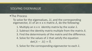
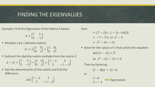
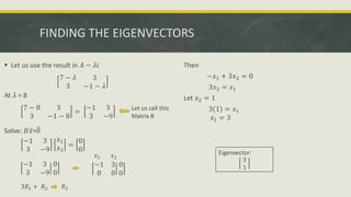
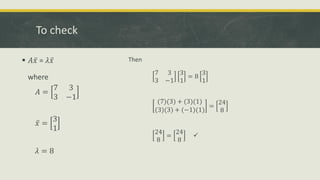
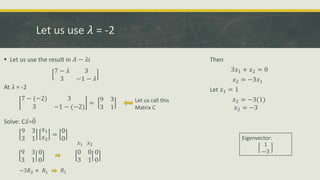
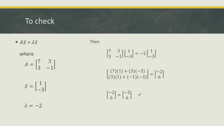
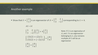
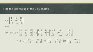
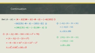
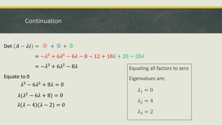
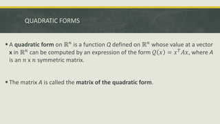
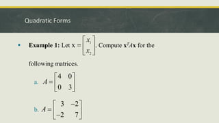
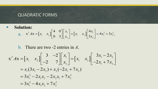
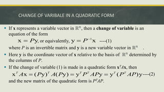
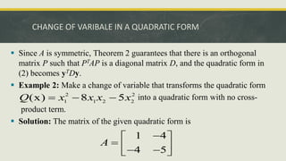
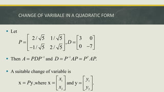
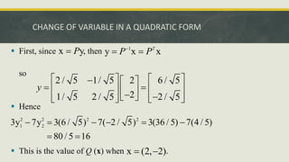
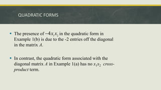
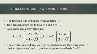
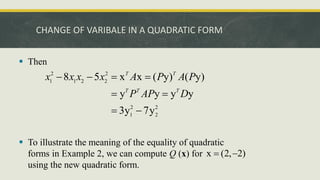
This document discusses eigenvalues, eigenvectors, and quadratic forms. It provides examples of how to: - Find the eigenvalues and eigenvectors of a matrix by solving the characteristic equation. - Express a quadratic form in terms of a matrix and change variables using an invertible matrix to diagonalize the quadratic form. - Use orthogonal diagonalization to transform a quadratic form with cross-product terms into one without cross-product terms. Step-by-step solutions and explanations are provided for examples involving 2x2 and 3x3 matrices.

1. Eigenvalue Problems and
Quadratic Forms
ENGINEERING MATHEMATICS
By: Engr. Angelo Ramos, LPT, MEng

2. What is EIGENVALUE
Definition
A scalar associated with a given linear transformation
of a vector space and having the property that there is
some nonzero vector which when multiplied by the
scalar is equal to the vector obtained by letting the
transformation operate on the vector; especially: a
root of the characteristic equation of a matrix.
German word – Eigenwert, eigen means “own”; wert
means “value”.

3. EIGENVALUE and EIGENVECTOR
A scalar 𝜆 is called an eigenvalue of an
𝑛 x 𝑛 Matrix 𝐴 if there is a nonzero
vector ҧ
𝑥 such that 𝐴 ҧ
𝑥 = 𝜆 ҧ
𝑥. Such a
vector ҧ
𝑥 is called an eigenvector of 𝐴
corresponding to 𝜆.

4. Solving Eigenvalue

5. SOLVING EIGENVALUE
Let 𝐴 be an 𝑛 x 𝑛 matrix. 𝐴 scalar 𝜆 (lambda)
is called an eigenvalue of 𝐴 if there is
nonzero vector ҧ
𝑥 such that 𝐴 ҧ
𝑥 = 𝜆 ҧ
𝑥. Such a
vector ҧ
𝑥 is called an eigenvector to 𝜆.

6. SOLVING EIGENVALUE
The Process
To solve for the eigenvalues, 𝜆𝑖, and the corresponding
eigenvector, ҧ
𝑥𝑖 of an 𝑛 x 𝑛 matrix 𝐴, do the following:
1. Multiply an 𝑛 x 𝑛 identity matrix by the scalar 𝜆.
2. Subtract the identity matrix multiple from the matrix 𝐴.
3. Find the determinants of the matrix and the difference.
4. Solve for the values of 𝜆 that satisfy the equation
det 𝐴 − 𝜆i = ത
0.
5. Solve for the corresponding eigenvector to each 𝜆.

7. FINDING THE EIGENVALUES
Example: Find the Eigenvalue of the Matrix A below
𝐴 =
7 3
3 −1
 Multiply 𝜆 by 𝑖 (identity matrix)
𝜆𝑖 = 𝜆
1 0
0 1
=
𝜆 0
0 𝜆
 Subtract the identity matrix multiple from the matrix 𝐴
𝐴 − 𝜆𝑖 =
7 3
3 −1
−
𝜆 0
0 𝜆
=
7 − 𝜆 3
3 −1 − 𝜆
 Get the determinants of the matrix and find the
difference.
d𝑒𝑡
7 − 𝜆 3
3 −1 − 𝜆
then
= (7 − 𝜆)(− 1 − 𝜆) −(3)(3)
= −7 − 7𝜆+ 𝜆+ 𝜆2
− 9
= 𝜆2
− 6𝜆 − 16
 Solve for the values of 𝜆 that satisfy the equation
det 𝐴 − 𝜆i = ത
0
So 𝜆2
− 6𝜆 − 16 = 0
Then by factoring
(𝜆 − 8)(𝜆 + 2) = 0
ie:
𝜆 = 8
𝜆 = − 2
Eigenvalues

8. FINDING THE EIGENVECTORS
 Let us use the result in 𝐴 − 𝜆𝑖
7 − 𝜆 3
3 −1 − 𝜆
At 𝜆 = 8
7 − 8 3
3 −1 − 8
=
−1 3
3 −9
Solve: 𝐵 ҧ
𝑥=ത
0
−1 3
3 −9
𝑥1
𝑥2
=
0
0
ቚ
−1 3
3 −9
0
0
Then
−𝑥1 + 3𝑥2 = 0
3𝑥2 = 𝑥1
Let 𝑥2 = 1
3(1) = 𝑥1
𝑥1 = 3
Let us call this
Matrix B
3𝑅1 + 𝑅2 𝑅2
ቚ
−1 3
0 0
0
0
𝑥1 𝑥2
Eigenvector:
3
1

9. To check
 𝐴 ҧ
𝑥 = 𝜆 ҧ
𝑥
where
𝐴 =
7 3
3 −1
ҧ
𝑥 =
3
1
𝜆 = 8
Then
7 3
3 −1
3
1
= 8
3
1
(7)(3) + (3)(1)
(3)(3) + (−1)(1)
=
24
8
24
8
=
24
8


10. Let us use 𝜆 = -2
 Let us use the result in 𝐴 − 𝜆𝑖
7 − 𝜆 3
3 −1 − 𝜆
At 𝜆 = -2
7 − (−2) 3
3 −1 − (−2)
=
9 3
3 1
Solve: C ҧ
𝑥=ത
0
9 3
3 1
𝑥1
𝑥2
=
0
0
ቚ
9 3
3 1
0
0
Then
3𝑥1 + 𝑥2 = 0
𝑥2 = −3𝑥1
Let 𝑥1 = 1
𝑥2 = −3(1)
𝑥2 = −3
Let us call this
Matrix C
−3𝑅2 + 𝑅1 𝑅1
ቚ
0 0
3 1
0
0
𝑥1 𝑥2
Eigenvector:
1
−3

11. To check
 𝐴 ҧ
𝑥 = 𝜆 ҧ
𝑥
where
𝐴 =
7 3
3 −1
ҧ
𝑥 =
1
−3
𝜆 = −2
Then
7 3
3 −1
1
−3
= −2
1
−3
(7)(1) + (3)(−3)
(3)(1) + (−1)(−3)
=
−2
6
−2
6
=
−2
6


12. Another example
 Show that ҧ
𝑥 =
2
1
is an eigenvector of 𝐴 =
3 2
3 −2
corresponding to 𝜆 = 4.
𝐴 ҧ
𝑥 = 𝜆 ҧ
𝑥
3 2
3 −2
2
1
= 4
2
1
3 2 + (2)(1)
3 2 + (−2)(1)
=
8
4
8
4
=
8
4
Note: If 𝜆 is an eigenvalue of
𝐴, and ҧ
𝑥 is an eigenvector
belonging to 𝜆, any nonzero
multiple of ҧ
𝑥 will be an
eigenvector

13. Find the Eigenvalue of this 3 x 3 matrix
𝐴 =
4 6 10
3 10 13
−2 −6 −8
Sol’n
Det 𝐴 − 𝜆𝑖 =
4 6 10
3 10 13
−2 −6 −8
− 𝜆
1 0 0
0 1 0
0 0 1
=
4 − 𝜆 6 10
3 10 − 𝜆 13
−2 −6 −8 − 𝜆
= 4 − 𝜆
10 − 𝜆 13
−6 −8 − 𝜆
− 6
3 13
−2 −8 − 𝜆
+ (10)
3 10 − 𝜆
−2 −6

14. Det 𝑨 − 𝝀𝒊 = 𝟒 − 𝝀 𝟏𝟎 − 𝝀 −𝟖 − 𝝀 − −𝟔 𝟏𝟑
− 𝟔 𝟑 −𝟖 − 𝝀 − 𝟏𝟑 −𝟐
+(𝟏𝟎) 𝟑 −𝟔 − (−𝟐)(𝟏𝟎 − 𝝀
Continuation
(4 − 𝜆)(−80 − 10𝜆 + 8𝜆 + 𝜆2
+ 78)
= (4 − 𝜆)(−2 − 2𝜆 + 𝜆2
)
= −8 − 8𝜆 + 4𝜆2 + 2𝜆 + 2𝜆2 − 𝜆3
= −𝜆3
+ 6𝜆2
− 6𝜆 − 8




(−6)(−24 − 3𝜆 + 26)
= (−6)(2 − 3𝜆)
= −12 + 18𝜆

(10)(−18 + 20 − 2𝜆)
= (10)(2 − 2𝜆)
= 20 − 20𝜆


15. Det 𝑨 − 𝝀𝒊 = + +
= −𝜆3
+ 6𝜆2
− 6𝜆 − 8 − 12 + 18𝜆 + 20 − 20𝜆
= −𝜆3 + 6𝜆2 − 8𝜆
Equate to 0
𝜆3
− 6𝜆2
+ 8𝜆 = 0
𝜆(𝜆2
− 6𝜆 + 8) = 0
𝜆(𝜆 − 4)(𝜆 − 2) = 0
Continuation
 

Equating all factors to zero
Eigenvalues are:
𝜆1 = 0
𝜆2 = 4
𝜆3 = 2

16. Quadratic Forms

17. QUADRATIC FORMS
 A quadratic form on ℝ𝑛 is a function Q defined on ℝ𝑛 whose value at a vector
x in ℝ𝑛
can be computed by an expression of the form 𝒬 𝑥 = 𝑥𝑇
𝐴𝑥, where A
is an 𝑛 x 𝑛 symmetric matrix.
 The matrix A is called the matrix of the quadratic form.

18. Quadratic Forms
 Example 1: Let . Compute xTAx for the
following matrices.
a.
b.
1
2
x
x
x
 
  
 
4 0
0 3
A
 
  
 
3 2
2 7
A

 
  

 

19. QUADRATIC FORMS
 Solution:
a. .
b. There are two -2 entries in A.
   
1 1 2 2
1 2 1 2 1 2
2 2
4
4 0
x x 4 3
3
0 3
T
x x
A x x x x x x
x x
   
 
   
   
 
     
   
1 1 2
1 2 1 2
2 1 2
1 1 2 2 1 2
2 2
1 1 2 2 1 2
2 2
1 1 2 2
3 2
3 2
x x
2 7
2 7
(3 2 ) ( 2 7 )
3 2 2 7
3 4 7
T
x x x
A x x x x
x x x
x x x x x x
x x x x x x
x x x x

    
 
 
   
   

     
    
   
  

20. QUADRATIC FORMS
 The presence of in the quadratic form in
Example 1(b) is due to the -2 entries off the diagonal
in the matrix A.
 In contrast, the quadratic form associated with the
diagonal matrix A in Example 1(a) has no x1x2 cross-
product term.
1 2
4x x


21. CHANGE OF VARIBALE IN A QUADRATIC FORM
 If x represents a variable vector in ℝ𝑛
, then a change of variable is an
equation of the form
, or equivalently, ----(1)
where P is an invertible matrix and y is a new variable vector in ℝ𝑛 .
 Here y is the coordinate vector of x relative to the basis of ℝ𝑛 determined by
the columns of P.
 If the change of variable (1) is made in a quadratic form xTAx, then
----(2)
and the new matrix of the quadratic form is PTAP.
x y
P
 1
y x
P

x x ( y) ( y) y y y ( )y
T T T T T T
A P A P P AP P AP
  

22. CHANGE OF VARIBALE IN A QUADRATIC FORM
 Since A is symmetric, Theorem 2 guarantees that there is an orthogonal
matrix P such that PTAP is a diagonal matrix D, and the quadratic form in
(2) becomes yTDy.
 Example 2: Make a change of variable that transforms the quadratic form
into a quadratic form with no cross-
product term.
 Solution: The matrix of the given quadratic form is
2 2
1 1 2 2
(x) 8 5
Q x x x x
  
1 4
4 5
A

 
  
 
 

23. CHANGE OF VARIBALE IN A QUADRATIC FORM
 The first step is to orthogonally diagonalize A.
 Its eigenvalues turn out to be 𝜆 = 3 and 𝜆 = −7 .
 Associated unit eigenvectors are
 These vectors are automatically orthogonal (because they correspond to
distinct eigenvalues) and so provide an orthonormal basis for ℝ2 .
2 / 5 1/ 5
λ 3: ;λ 7 :
1/ 5 2 / 5
   
  
   

   
   

24. CHANGE OF VARIBALE IN A QUADRATIC FORM
 Let
 Then and .
 A suitable change of variable is
,where and .
2 / 5 1/ 5 3 0
,
0 7
1/ 5 2 / 5
P D
   
 
   

  
 
 
1
A PDP
 1 T
D P AP P AP

 
x y
P
 1
2
x
x
x
 
  
 
1
2
y
y
y
 
  
 

25. CHANGE OF VARIBALE IN A QUADRATIC FORM
 Then
 To illustrate the meaning of the equality of quadratic
forms in Example 2, we can compute Q (x) for
using the new quadratic form.
2 2
1 1 2 2
2 2
1 2
8 5 x x ( y) ( y)
y y y y
3y 7y
T T
T T T
x x x x A P A P
P AP D
   
 
 
x (2, 2)
 

26. CHANGE OF VARIABLE IN A QUADRATIC FORM
 First, since , then
so
 Hence
 This is the value of Q (x) when .
x y
P
 1
y x x
T
P P

 
2 / 5 1/ 5 2 6 / 5
2
1/ 5 2 / 5 2 / 5
y
   
  
 
   
 
 
 
   
   
2 2 2 2
1 2
3y 7y 3(6 / 5) 7( 2 / 5) 3(36 / 5) 7(4 / 5)
80 / 5 16
     
 
x (2, 2)
 