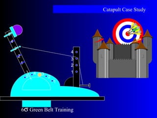
2. Catapult Exercise
• You have been pre-selected (based on your skills and past performance
records) for the openings posted for Her Majesty’s Catapult Squad.
• Problem Statement: Catapult launching is not capable of meeting Her
Majesty’s requirements over the target range of 5-12 feet +/- 6 inches.
• Goal: Your mission is to optimize the inputs to be able to hit a target
repeatedly within this range so that Her Majesty can conquer the evil Empire.
• A successful catapult squad can place a payload to the target every time.
(Only 3.4 misses per million!)
• The distance from the target varies due to several factors; consequently, you
don’t know the distance until you’re in position.
• May the FORCE be with You!! Heads rolled on the last crew which is why
we have postings for the current positions!
3. Project DefinitionProject Definition
Problem Statement:
Catapult launching is not capable of
meeting Her Majesty’s requirements over
the target range of 5-12 feet +/- 6 inches.
CTS’s:
Target distance (5 to 12 feet)
Consistency (+/- 6 inches)
Speed (rapid set up and launch capability)
Defect Definition:
Payloads outside of the target specification
Metrics:
Distance (inches)
Standard deviation (inches)
Project Objective:
To develop a standard process and y = f(x)
equation so that the catapult can be shot to
meet the customer requirements (distance)
and minimize variation (< 6 inch radius).
Current/Goal/Stretch Goal
Current DPMO/Zst - TBD
Goal DPMO/Zst - TBD
Benefits:
• improved accuracy
• reduced variation
• customer satisfaction
• we live!
Progress to Date:
• Team members selected
4. Catapult Nomenclature
Rubber band
attachment point
Rubber band
attachment point Arm stop positionArm stop position
Front arm tension
point
Front arm tension
point
1
2
34
5
1
2
3
4
5
1
2
3
4
Draw-back angleDraw-back angle
Ball typeBall type
Cup locationCup location
Number of rubber
bands
Number of rubber
bands
5. Update RecommendedUpdate Recommended
Actions To DateActions To Date
Description of
potential Root cause
or potential vital X
What leads me to
believe this is a
potential X (Data,
local knowledge,
Oberservation, Tool?)
What change is being
proposed to the X to
possibly generate a
process improvement
To be tested (team
agreement)
Rubber band C&E Matrix, FMEA Constant time between
shots
No
Operator C&E Matrix, FMEA ANOVA
Equal Variances
Evaluate using previous
data
Standard Operating
Procedures
There currently is none An SOP was
implemented to
stabilize the launches
Create prior to
Hypothesis Testing
and/or DOE
Ball type C&E Matrix, FMEA Test the ball type in a 2
sample t-test
Equal Variance Test
Yes
6. Step 7: Screen PotentialStep 7: Screen Potential
CausesCauses
Narrow it Down
Screening is done using Graphical Tools,
Experiments, and Hypothesis Tests to identify
and prove which are the vital X’s
This is the middle of the funnel for most
projects (multiple X’s or with variable
relationships between X’s)
– for some simpler projects with a single X, this is the
bottom of the funnel, the final vital X
Important X’s for Y = f(X1, X2, …, Xn) – we still need to determine “f”
7. Hypothesis Testing ForHypothesis Testing For
Sources of VariationSources of Variation
What potential sources of variation can be
explored using Hypothesis Testing ?
What are sources of data that can be analyzed
– Passive: existing data
– Active: sampling the process
Ball Type
– Whiffle versus Ping Pong?
Mean or variation?
Catapult Setup – Floor type
– Table top or floor? Tile or carpet?
Mean or variation?
8. Update RecommendedUpdate Recommended
Actions To DateActions To Date
Description of
potential Root cause
or potential vital X
What leads me to
believe this is a
potential X (Data,
local knowledge,
Oberservation, Tool?)
What change is being
proposed to the X to
possibly generate a
process improvement
To be tested (team
agreement)
Ball Type 2 sample t-test
Equal Variance
DOE – test 2 different
types
Completed
Draw Back Angle C&E Matrix, and
FMEA
DOE – test 2 different
settings
Yes
Front Tension Pin C&E Matrix, and
FMEA
DOE – test 2 different
settings
Yes
Rubber band C&E Matrix FMEA Time between shots No
Operator 2 sample t-test 1 operator for DOE No
Standard Operating
Procedures
There currently is none An SOP was
implemented to
stabilize the launches
Not at this time; SOP’s
to be applied in DOE
Pin Height C&E Matrix, FMEA DOE – test 2 different
settings
Yes
9. 22KK
Full Factorial Design ofFull Factorial Design of
ExperimentsExperiments
Catapult ExerciseCatapult Exercise
10. The Breakthrough StrategyImproveThe Breakthrough StrategyImprove
1. Select Output Characteristics
2. Define Performance Standards
3. Validate Measurement System
4. Establish Process Capability
5. Define Performance Objectives
6. Identify Variation Sources
7. Screen Potential Causes
8. Discover Variable Relationships
9. Establish Operating Tolerances
10.Validate Measurement System
11.Determine Process Capability
12.Implement Process Controls
11. Step 8: Discover VariableStep 8: Discover Variable
RelationshipsRelationships
How the X’s affect Y
Evaluate how my Vital X’s affect Y, either
independently or in combination with other
Vital X’s. This is primarily done through the
use of DOE or Regression.
This is the bottom of the funnel, I know which
X’s affect my Y and I know how they affect Y
The function Y = f(X1, X2,…, Xn) is called a
“transfer function” – it describes how a change
in one or more of the X’s transfers to a change
in Y
We now know what Y = f(X1, X2, …, Xn) is
The variable relationships within many Green Belt projects are frequently
established simply through the use of standard hypothesis tests.
12. Step 9: Establish OperatingStep 9: Establish Operating
TolerancesTolerances
How To Set My Xs
I know which X’s are important. What settings
do I use to improve my project?
In the case of a variable X (e.g. PSI on an air
feed), I have to provide a setting tolerance (e.g.
a target amount ± an allowed amount of
variation about the target)
In the case of a non-variable X (e.g. Supplier), I
know which value of the variable provides the
best value of Y, therefore I have specified the
absolute operating tolerance
Make use of what we know about Y = f(X1, X2, …, Xn)
In our case study we will “set the X’s” at the
settings of our improved process.
13. Improve PhaseImprove Phase
We will conduct a 2k
factorial experiment in order
to identify the proper factors and levels to achieve
the highest capability (Zst).
– You only have enough resources to investigate three
X’s at 2 levels
– Determine your factors and their respective levels.
– Use the knowledge you learned in DMA and as a team
determine what factors and the respective levels you
want to use to conduct the DOE
14. Philosophy of ExperimentationPhilosophy of Experimentation
Catapult
Process
Responses
Distance
Variation
Controllable X’s
Draw Back Angle
Fr Arm Tension
Stop Pin
Uncontrollable X’s
“Noise”
Adjustment X’s
“SOP’s”
Temp Air flowDistractions
Setup Ball Type
ReleaseOperator
15. Step 2: Factors, Level SettingsStep 2: Factors, Level Settings
and Sample Sizeand Sample Size
Use the Strategy for Experimentation to complete the following:
Conduct a 3 factor, 2 level full factorial design with 6 repeats to optimize the
catapult settings to hit a target within +/- 6”
Factors: A: Stop Pin: 2 and 4
B: Draw back angle: 140 and 180
C: Front Tension Pin: 2 and 4
16. Step 4: Create The Design InStep 4: Create The Design In
MinitabMinitab
Stat>DOE>Factorial>Create Factorial
Design
• Select the number of factors (3)
• Open the ‘Designs…’ window
• Highlight the ‘Full Factorial’
• Maintain all other defaults
• OK
17. Creating The Design, Cont’dCreating The Design, Cont’d
• Un-check the ‘Randomize runs’ box
• OK
• Enter Factor Names
• Enter Factor Low & High Settings
• OK
18. Resultant Design In The WorksheetResultant Design In The Worksheet
Session Window Output:
Factorial Design
Full Factorial Design
Factors: 3 Base Design: 3, 8
Runs: 8 Replicates: 1
Blocks: none Center pts (total): 0
All terms are free from aliasing
Worksheet Output:
19. Step 5: Conduct The ExperimentStep 5: Conduct The Experiment
Populate the worksheet with the results
of your experiment and calculate the
Row Averages and Row Standard Deviations:
AvrgD Calculation: Calc>Row Statistics,
Check ‘Mean’, Input Variables: ‘Y1 through Y6’,
Store Result in: ‘AvrgD’
SD Calculation: Calc>Row Statistics, Check
‘Standard deviation’, Input Variables: ‘Y1
through Y6’, Store Result in: ‘SD’
CATAPULT Round 5 DOE
Example.mtw
22. AvrgD: Main Effects PlotAvrgD: Main Effects Plot
Which factor has the greatest effect on the
Average Distance?
StopPin DrawAngle TensionPin
2 4 140
180
2 4
40
50
60
70
80
AvrgD
Main Effects Plot (data means) for AvrgD
23. AvrgD: Interaction PlotAvrgD: Interaction Plot
There appears to be one potential interaction:
– StopPin*DrawAngle
– The effect that Stop Pin has on Distance also depends
on the Draw Back Angle
140
180
2 4
20
60
100
20
60
100
StopPin
DrawAngle
TensionPin
2
4
140
180
Interaction Plot (data means) for AvrgD
24. AvrgD: Cube PlotAvrgD: Cube Plot
Is a distance of 70” achievable with the
Tension Pin at setting 2?
Is a distance of 50” achievable with the
Draw Back Angle at 140?
36.00
59.83
60.54
93.25
15.50
33.13
63.50
109.63
2 4
StopPin
DrawAngle
TensionPin
140
180
2
4
Cube Plot (data means) for AvrgD
25. Step 6: Perform TheStep 6: Perform The
DOE Analysis For TheDOE Analysis For The
Full ModelFull Model
Stat>DOE>Factorial>Analyze Factorial
Design:
26. Step 6: Full Model AnalysisStep 6: Full Model Analysis
Cont’dCont’d
27. Running the Full ModelRunning the Full Model
0 10 20 30 40
AC
ABC
A
BC
AB
C
B
Pareto Chart of the Effects
(response is AvrgD, Alpha = .10)
A: StopPin
B: DrawAngl
C: TensionP
• With all terms in the model, only one appears above the significance
level (red line)
28. Step 8: Reducing The ModelStep 8: Reducing The Model
0 5 10
A
BC
AB
C
B
Pareto Chart of the Standardized Effects
(response is AvrgD, Alpha = .10)
A: StopPin
B: DrawAngl
C: TensionP
0 1 2 3 4 5 6 7
A
AB
C
B
Pareto Chart of the Standardized Effects
(response is AvrgD, Alpha = .10)
A: StopPin
B: DrawAngl
C: TensionP
29. AvrgD: Final Reduced ModelAvrgD: Final Reduced Model
Estimated Effects and Coefficients for AvrgD (coded units)
Term Effect Coef SE Coef T P
Constant 58.922 3.091 19.06 0.000
StopPin 6.969 3.484 3.091 1.13 0.342
DrawAngl 45.615 22.807 3.091 7.38 0.005
TensionP 30.073 15.036 3.091 4.87 0.017
StopPin*DrawAngl -16.635 -8.318 3.091 -2.69 0.074
Analysis of Variance for AvrgD (coded units)
Source DF Seq SS Adj SS Adj MS F
P
Main Effects 3 6067.3 6067.3 2022.42 26.47
0.012
2-Way Interactions 1 553.5 553.5 553.47 7.24
0.074
Residual Error 3 229.2 229.2 76.42
Total 7 6850.0
Estimated Coefficients for AvrgD using data in uncoded units
Term Coef
Constant -378.724
StopPin 70.0260
DrawAngl 2.38802
TensionP 15.0365
StopPin*DrawAngl -0.415885
Use the uncoded
coefficients to create
the equation
30. Creating the y = f(x) for AvrgDCreating the y = f(x) for AvrgD
Create the equation from the un-coded
coefficients:
AvrgDuncoded = -378.72 + 70.03 * StopPin + 2.39
* DrawAngle + 15.04 * TensionPin - 0.42 *
StopPin*DrawAngle
Estimated Coefficients for AvrgD using data in uncoded units
Term Coef
Constant -378.724
StopPin 70.0260
DrawAngl 2.38802
TensionP 15.0365
StopPin*DrawAngl -0.415885
31. Setting Pin Positions To Minimize VariationSetting Pin Positions To Minimize Variation
Given a target of 60”,
where would you set the
pin positions to
minimize variation?
3.118
2.463
6.026
14.716
0.548
2.011
1.844
3.694
2 4
StopPin
DrawAngle
TensionPin
140
180
2
4
Cube Plot (data means) for SD
36.00
59.83
60.54
93.25
15.50
33.13
63.50
109.63
2 4
StopPin
DrawAngle
TensionPin
140
180
2
4
Cube Plot (data means) for AvrgD
Settings at approx. 60”
There are 4 possible
combinations to hit the
target. Which one
minimizes variation?
32. Recommended Pin Factor Level SettingsRecommended Pin Factor Level Settings
Stop Pin: 2
Front Tension Pin: 2
Recall the equation for AvrgD:
– AvrgD = -378.7 + 70.03 * StopPin + 2.39 * DrawAngle +
15.04 * TensionPin - 0.42 * StopPin*DrawAngle
Enter the fixed settings into the equation for AvrgD:
– AvrgD = -378.7 + (70.03 * 2) + 2.39 * DrawAngle + (15.04 *
2) - 0.42 * (2*DrawAngle)
Reduce the equation:
– AvrgD = -378.7 + 140.06 + 2.39 * DrawAngle + 30.08 - 0.84
* DrawAngle
– AvrgD = -208.6 + 1.55*DrawAngle
Substitute the target (60”) for AvrgD and solve for Draw Angle
– DrawAngle = 173.3 degrees
33. Okay… Your Turn!Okay… Your Turn!
Round #5: DOERound #5: DOE
Open the DOE design in Minitab:
– CATAPULT Round 5 DOE Worksheet.mtw
Conduct the experiment and record the data
Analyze the experiment
– Graphically
– Analytically
Obtain a prediction equation for Distance
Present your cube plots to the instructor to receive your target
Obtain a target value from the instructor
Establish Pin factor levels based on goal to minimize variation
Conduct a validation run
– Launch 10 shots using the predicted settings
Calculate the mean and standard deviation
Flipchart your results
34. Catapult Nomenclature
Rubber band
attachment point
Rubber band
attachment point Arm stop positionArm stop position
Front arm tension
point
Front arm tension
point
1
2
34
5
1
2
3
4
5
1
2
3
4
Draw-back angleDraw-back angle
Ball typeBall type
Cup locationCup location
Number of rubber
bands
Number of rubber
bands
35. Step 10: Validate MeasuringStep 10: Validate Measuring
SystemSystem
Can I Measure My Xs & Y?
In the case of a variable X (e.g. PSI on an air
feed), I need to validate that it can be measured
(a vital X MSA)
In the case of a non-variable X, I need to
validate that I can tell whether the X is the right
value (e.g. is this from Supplier A?)
Also, I might have improved my Y so much
that I can no longer “read” my process, and may
have to improve my measurement system to
truly measure the improvement
Can’t control Y = f(X1, X2, …, Xn) if you can’t measure it
36. Case Study 2: The CatapultCase Study 2: The Catapult
Control
37. The Breakthrough StrategyThe Breakthrough Strategy
ControlControl
1. Select Output Characteristics
2. Define Performance Standards
3. Validate Measurement System
4. Establish Process Capability
5. Define Performance Objectives
6. Identify Variation Sources
7. Screen Potential Causes
8. Discover Variable Relationships
9. Establish Operating Tolerances
10. Validate Measurement System
11. Determine Process Capability
12. Implement Process Controls
38. Case Study 2: The CatapultCase Study 2: The Catapult
Final Capability
39. Step 11: Determine Process CapabilityStep 11: Determine Process Capability
Where Am I?
This measures the capability of controlling my
Xs at their optimal settings
This is also the time when we determine formal
results by comparing a new capability analysis
with the baseline capability analysis (step 4)
and our goals (step 5)
Common tools:
– Six Sigma Capability Analysis (Normal) for
continuous data
– Six Sigma “Product Report” for discrete data
Can you consistently make X1, X2, …, Xn to produce “good” Y’s?
For our case study, we will rerun the Capability Analysis in
MINITAB using our new process to see before and after.
40. Improved CapabilityImproved Capability
Method 1 – Capability Analysis (NormalMethod 1 – Capability Analysis (Normal))
Based on the Project work conducted by the
team, shown below is the improved
capability.
30 35 40 45 50
LSL USL
Process Capability Analysis for Improved Dis
USL
Target
LSL
Mean
Sample N
StDev (Within)
StDev (Overall)
Z.Bench
Z.USL
Z.LSL
Cpk
Cpm
Z.Bench
Z.USL
Z.LSL
Ppk
PPM < LSL
PPM > USL
PPM Total
PPM < LSL
PPM > USL
PPM Total
PPM < LSL
PPM > USL
PPM Total
41.0000
*
37.0000
38.9405
100
0.392507
0.416816
4.91
5.25
4.94
1.65
*
4.61
4.94
4.66
1.55
0.00
0.00
0.00
0.38
0.08
0.46
1.62
0.39
2.00
Process Data
Potential (Within) Capability
Overall Capability Observed Performance Exp. "Within" Performance Exp. "Overall" Performance
Within
Overall
41. Case Study ExerciseCase Study Exercise
Round #6: Process CapabilityRound #6: Process Capability
Objective: To determine Capability for your improved process
–Catapult settings based on:
Optimum conditions from the DOE
Results from validation run
SOP’s
–Each of 5 Operators will launch 5 balls at a time
–Alternate Operators until you have launched 50 balls
–Enter into: Catapult Round 6 Cap Worksheet.mtw
–Generate the Process Capability (Normal) using n=5
Deliverable: Using the table on the following page, record on a flip chart the following for
your team
– Final Average, inches
– Final Standard deviation, inches
– Final Short term capability (Zst)
– Final DPMO
Time: 30 minutes
42. Catapult Project MetricsCatapult Project Metrics
Parameter Team 1 Team 2 Team 3 Team 4 Team 5
BASELINE
Average, in.
St. Dev., in.
Zst
DPMO
Objective DPMO
FINAL
Average, in.
St. Dev., in.
Zst
DPMO
% Reduction in DPMO
43. Step 12: Implement ProcessStep 12: Implement Process
ControlsControls
Let’s Not Do This Again
The X’s you have determined as vital, their
settings, and other actions you have taken to
make the improvement must be:
– nailed down
– set in concrete
– fully implemented (NOT just agreed to)
– put into a rigorous audit schedule
– Documented in a Control Plan
BEFORE you can say a project is closed!
How do you control X1, X2, …, Xn to always produce “good” Y’s?
44. Controls – Two RequirementsControls – Two Requirements
1) The actual controls
Controls must be placed on completed projects to make
sure that they do not decay – Energy must be expended on
processes to keep them in their optimum condition.
– The degree of control is proportional to the risk of the
process decaying from its final project derived settings.
2) The Control Plan
The controls must be documented carefully, answering:
– What is being done?
– Who is to do it (position not name of person)?
– When is to be done?
– What will be action if process does decay?
– What will make it difficult to change the project settings OR
controls?
“If it isn’t written down, It doesn’t exist”
45. Case Study 2: The CatapultCase Study 2: The Catapult
SPC, Variable Data
46. Why Use SPC for Variables?Why Use SPC for Variables?
SPC for variable data is used to:
Keep process centered
Minimize variation
Reduce excursions
Validate improvements
Focus Six Sigma®
process activity
47. What is SPC for Variables?What is SPC for Variables?
SPC for variable data is
Industry standard control language
Reliable, easy method of determining
– Common cause variation
– Special cause variation
Graphical communication
Set of statistical tools for analyzing variables
performance data
Statistical Process Control
Is application of statistical tools and methods to
provide feedback
Sets limits of variation
Provides trigger for action
48. SPC FunctionSPC Function
SPC Charts
Used to monitor and control process under
local responsibility
Require process owners to
– take measurements
– Plot and interpret data
– Take action
Provide a history of the process
49. Components of a ControlComponents of a Control
ChartChart
10
9
8
7
6
5
4
3
2
1
0
0 5 10 15 20
Upper Control
Limit
Lower Control
Limit
Mean
Nonrandom Variation Region
‘Special Cause Variation’
Observation number
Observationvalue
Random Variation Region
‘Common Cause Variation’Observation 10
50. Statistics of a Control ChartStatistics of a Control Chart
10
9
8
7
6
5
4
3
2
1
0
0 5 10 15 20
Nonrandom Variation Region
Observation number
Observationvalue
Random Variation Region
LCL
- 3σ
UCL
+ 3σ
Mean
99.73%
area
51. Establishing Process ControlEstablishing Process Control
LimitsLimits
Control limits are
Are statistical limits set +/- 3 standard deviations
from the mean
Set when process is in control
– Fixed at baseline value
– Adjusted for improvements
– Never widened
Control limits are not related to specification
limits
Control Limits are not specification limits
52. Definition of ControlDefinition of Control
In control is
A statistical term for process variation
– Within three standard deviations of the mean
– That is random without cause
– That does not show run patterns
– That does not show trend patterns
No assignable cause variation
53. Control Chart RoadmapControl Chart Roadmap
Variable
Data
Xbar-R
Chart
I-MR
Chart
Xbar-s
chart
N<10
No
Yes
N=1
NoYes
54. Xbar-R Chart PrinciplesXbar-R Chart Principles
Xbar-R Charts (and Xbar-s) are two separate charts
of the same subgroup data
Xbar chart is a plot of the subgroup means
R chart is a plot of the subgroup ranges (or if s,
plot of subgroup standard deviation)
Most sensitive charts for tracking and identifying
assignable cause of variation
Based on control chart factors that assume a
normal distribution within subgroups
Establish three sigma process limits
55. Xbar-R Chart ExerciseXbar-R Chart Exercise
Open the Minitab file: Catapult Variable
SPC Example.mtw
This was a teams’ initial (Round 3)
capability study
5 operators launched 5 shots each
– Sequence was repeated 4 times
– Total observations: 100
58. Exercise: Catapult Xbar-R ChartsExercise: Catapult Xbar-R Charts
Individually with your team, plot your Catapult
capability data from Round #6
Create the standard Xbar-R chart
– Is your process in control?
Sort the data by Operator
Create a Xbar-R chart with control limits by ‘Operator’
– Is there a visual difference between operators with respect to
Central tendency?
Variation?
– Are they individually in control?
What happens to the control chart if the subgroup size is
the total number of shots per operator?
59. I-MR Chart PrinciplesI-MR Chart Principles
Individual and Moving Range Charts are two
separate charts of the same data
I chart is a plot of the individual data
MR chart is a plot of the moving range of the
previous individuals
I-MR charts are sensitive to trends, cycles and
patterns
Used when subgroup variation is zero or no
subgroups exist
– Destructive testing
– Batch processing
60. Example: How to Create an I-MR ChartExample: How to Create an I-MR Chart
Stat>Control Charts>I-MR…
61. Example I-MR ChartExample I-MR Chart
Compare this chart to the Xbar-R chart
0Subgroup 50 100
30
40
50
IndividualValue
1
1
1
1
1
Mean=38.65
UCL=43.97
LCL=33.33
0
5
10
MovingRange
1
1 1
1
1
R=2
UCL=6.535
LCL=0
I and MR Chart for Dist.
62. SPC ExerciseSPC Exercise
Catapult Variable SPC Example II.mtwCatapult Variable SPC Example II.mtw
A catapult team decided that they needed to be
able to control the Draw Back Angle.
An observer requested an operator to launch
consecutive balls at an angle of 180 degrees.
The observer, through special visual imaging
equipment, recorded the angle and the distance of
each launch.
Is the operator able to control the angle?
Generate a control chart and flip chart your
response.
63. Case Study 2: The CatapultCase Study 2: The Catapult
Audit
64. Catapult Control Plan ExerciseCatapult Control Plan Exercise
Purpose: To develop a Control Plan that sustains the gains of the work
our Six Sigma Team performed that optimizes the capability of the
catapult to deliver conforming product.
You and your Six Sigma team have have successfully completed a
project by identifying the critical X’s and their respective levels in order
to achieve your project objective.
It is now time to hand the project over to the Process Owner, therefore a
Control Plan needs to be developed. This Control Plan needs to contain
the proper information that will allow the Process Owner to sustain the
gains your team has achieved.
Any six sigma project must have a control plan
65. Catapult Control Plan FormCatapult Control Plan Form
Catapult Control Plan.pptCatapult Control Plan.ppt
KPOV KPIV
Measurement
Method
Who
Measures
Process Step Control Tool
KPIV/KPOV
Requirement
Specification/
Requirement
USL LSL
CTQ Sample
Size
Frequency
Where
Recorded
SOP Reference
Decision Rule/
Corrective Action
66. Optional Round #7: AuditOptional Round #7: Audit
Train a Replacement/Audit
Prove that your experimental results can sustain the test of time
over a broad inference space.
– Poke-Yoke your process so that it is robust to the many
operators that are likely to run the device.
– Your Crack Marketing Team received a letter from Her
Majesty in which she described the test as follows:
“The winning design will be the one that is able to launch ammunition
into a fine goblet from various distances.”
Further, the marketing team overheard that Her Majesty herself would
fire the catapult after a short tutorial from the gunsmith.
After you have completed the control plan and documented your SOP’s, I will
give you a new target to hit. You will have 5 minutes and 3 launches (within
those 5 minutes) to identify a new set of operating conditions. You will set up
the catapult at these new conditions. I will read your Standard Operating
Procedures and then launch 10 balls. The capability of these launches will be
included in the final competition calculations.
67. Case Study 2: The CatapultCase Study 2: The Catapult
Summary
68. Project Debriefs / SummaryProject Debriefs / Summary
Parameter Team 1 Team 2 Team 3 Team 4 Team 5
Baseline Zst
Final Zst
Baseline DPMO
Final DPMO
Baseline Average, in.
Final Average, in.
Baseline St. Dev., in.
Final St. Dev., in.
69. ReviewReview
In preparation for closing out your
project, include:
– Strategy, action plan and goals for the
project
– Tools and techniques used during the project
– Brief technical discussion of what was
learned by completing the project
– Brief discussion of team dynamics
Editor's Notes
This exercise has been compiled to allow participants in teams of 4-5 to complete a six sigma project from start to finish. The catapult may or may not be familiar to them. Assume they have NO experience with the catapult. Participants will be given certain elements of the project, such as process maps, fishbone diagrams, C&E diagrams, FMEA’s, etc. employing the catapults. Only pieces of the process have been assessed using six sigma tools up to this point. Recall that the process map, fishbone, C&E diagram and FMEA are NOT deliverables for this case study. This case study and the already prepared tools will eventually lead the teams/participants to select factors for the DOE.
Instructors have been assigned to provide one or more analogies for the Catapult Case Study; How does the Catapult Case Study relate to your specific organization. Introduce this analogy here and reinforce the analogy throughout the case study (various phases). It is very important that participants can relate the Catapult exercises to their projects and/or processes.
Communicate with the participants that they have just been drafted. They now represent teams or squads competing for this new position. I don’t think I would want to be the runner up in this case!
Upon completion of the DOE, each team will compete for Her Majesty’s Catapult Squad. Each team will be given a target and allowed three attempts to hit it. The team with the greatest number of direct hits and minimum variation will be considered the winners. Instructors may want to make up their own rules as they see fit.
Short and long term capability studies should be conducted based on a target of 11’. The target range, however, is between 5 and 12 feet with the competition target to be determined by the instructor. Don’t set as a goal 3 consecutive hits/this may get confusing.
Steps one and two have been completed. The goal is to hit a target and minimize variation of each shot about that target. Our problem statement and goal are clear but they have not been quantified. We’ve been told there is too much variation in the catapult process. We must be capable of hitting the target with the least amount of variation… Our lives depend upon it! What is our current level of performance? How capable are we of hitting any target, at this point?
Next steps: Determine what the current/baseline performance level is expressed in six sigma terms (DPMO and Z). These can be quantified with a capability study. The capability study will also allow us to establish our goal/objective; do we need to shift the mean, reduce variation or both.
Gosh, I had no idea that this contraption had so many moving parts controlled by so many pins. Certainly, it can’t be that difficult.
Instructor: Briefly review the catapult. It helps to have one at the front of the room so you can relate the physical attributes to the illustration and nomenclature given.
Note: Some catapults actually have six (6) cup attachment holes in the Draw back arm. If the instructions call for location 5, count from the bottom up as shown in the illustration above.
Be sure to take a test drive yourself with the prescribed catapult settings. Depending upon the amount of room you’ve been given to conduct the launches, you may have to change settings accordingly.
Instructors will need to physically verify the teams’ settings; there’s always one team that doesn’t follow instructions!
When attempting to solve problems, many people and teams, use a Cause and Effect diagram to generate ideas about the root cause. Unfortunately most people use this as a Solutions and Effect Diagram and never determine the true root cause. Ask yourself and the class, how can one implement a solution if we do not have data to support a root cause. The purpose of the table is for the participants to think about the potential root cause, how do they know it is a root cause, and what would they change.
Notice that the factors, Draw Back Angle, Stop Pin and Front Tension Pin are not on the list. Look to see that these variables are on there lists. Communicate that we will reserve these factors to test in the DOE. The potential KPIV’s addressed above are those that we think we can ‘adjust’ or ‘set’ to help us reduce variation. We are suggesting that the ball type can be determined by using a 2-sample t-test or paired t-test. A 2-sample t-test will allow us to calculate variation. An ANOVA can be applied to determine if there is a difference in the mean of the operator and an equal variance test to check for equal variances between operators. We can use the data from the initial capability to run the ANOVA. The capability test could be repeated after the SOP’s were developed to determine if we reduced variation between operators.
Teams will need at least 20 minutes to red-line the SOP’s to stabilize their process… process needs to be stable before the DOE.
Review recommended actions to date. It is possible that teams came up with different recommendations. They should have decided on at least the ball type.
Have the teams revisit their root cause table, especially the ‘to be tested’ elements. The remaining elements may fit nicely into our DOE. These include the draw back angle, the stop pin and the front tension pin.
Relate the intro w/ years of service; comparing a GB class in one location to another locations’ mean & variation. The discrete data of Stats background between classes used Chi Sq (demonstrated in Credit Card Case Study).
A common question after this slide is “Does this suggest we do OFAT experiments?”
Emphasize that hypothesis tests are conducted to screen some things that we ‘think’ are important. There is always a risk that a potential interaction (ie., ball type and pull back angle) may not be discovered. Once we think these factors are important, or have evidence to suggest that they are, we will conduct additional DOE’s or pilots to validate the results.
Initially, participants will not understand where they can apply Hypothesis testing. It’s important that the facilitator pull from not only the catapult exercise but their own personal applications within the industry.
Relate this to your organization/processes. Do you have existing data from the process available or do we have to go collect the data. Which method is better? Definitely, active data collection so that we know the integrity of the data. Use the catapult as an example. If data was collected pre-MSA, I’m not sure I’d trust it! However, trends in the data are probably correct and worth evaluating. Using existing data is considered ‘exploratory’ to help focus our efforts.
There may be other hypotheses that the teams may also reveal. The three above are most common. This section will explore different types of hypothesis tests for continuous, variable data for both the mean and variation. It is important that the teams relate the results to their objectives. Do they need to shift the mean, reduce variation or a combination of both?
Background on floor type: this could also be tile versus carpet. Some carpets have more ‘give’ or cushion than others, etc.
Review recommended actions to date. It is possible that teams came up with different recommendations. They should have decided on at least the ball type. Caution teams that they need to have considered some standard operating procedure to warm up the rubber band and be consistent with the time between shots. Release method is also very important.
Have the teams revisit their root cause table, especially the ‘to be tested’ elements. The remaining elements may fit nicely into our DOE.
Instructor needs to set up a spare catapult at the front of the training room in order to perform a short demonstration with the catapult and members from the audience. Fix the catapult to the table top; lay out a tape measure on the floor with foil beneath the tape measure.
Step 8: What is the y = f(x)?
Step 9: The DOE will allow us to determine the optimum for our x’s (factor level settings)
Step 10: Can we trust the x’s? Have we improved the process and reduced the overall process variation so much that we need to revisit the measurement system for the y? Reducing the 2total will make the %Contribution metric worse.
% Contribution = (2meas / 2total)x100
% Tolerance = 5.15(meas / Tolerance)x100
The Take Away states that this is where we now need to determine our transfer equation. Y is a function of which Xs.
The goal of the improve stage is to determine the y = f(x), properly tolerance the x’s and then validate the improvements.
We are actually going to apply Design of Experiments (DOE) to the catapult and construct an equation that will allow us to hit a target between 5-12 feet with minimum variation between repeated shots, if necessary!
How does this relate to the catapult; where do I need to set draw back angle and pin settings to achieve a distance of….
How much play or acceptable variation is in the draw back angle mechanism or the pin settings. Doesn’t it seem as though it would be much easier to control the variation in a pin setting than the draw back angle?
What things will contribute to variation in the pin settings? Wear of the pin, the holes in the wood, etc.
Give them the ‘big-picture.’ Where are we going from here, story-line. Make sure everyone is with you thus far.
In real life we do not have endless budgets. Processes and projects are constrained on many different resources. Experiments require lots of resources and often disrupt our processes, business processes and industrial processes. The team looked at there ‘No-budget’ six sigma project and decided they could only conduct a few experimental runs. It’s very important that they conduct their experiment efficiently.
Review briefly what we have learned on the catapult thus far.
The IPO (input, process, output) diagram depicts the inputs, process and outputs. We’ve now subdivided the types of inputs, based on our process knowledge, and key takeaway from the tools. There are factors that we have chosen to adjust or fix; these adjustment factors or SOP’s are a result of observation and hypothesis testing. For example, the set up and release methods were developed to minimize variation. The ball type was selected based on HT. The best operators were chosen based on the ANOVA, etc. We also recognize that there are factors that are out of our control or we chose not to control them, called noise factors. These include temperature, airflow, distractions in the room, etc. Then there are those controllable factors that ranked very high from the results of our FMEA that said, we should further study the effects of pull back angle, Front Pin Hgt and the Stop Pin position to ‘control’ the distance and variation of the ball about our target. Our goal is to now use these controllable factors in a Design of Experiment (DOE) to determine settings (x’s) to achieve our target (y’s). Essentially we want to construct the y = f(x).
The basis for experimentation is to discover something about a particular process or system.
Results and conclusions are dependent upon the manner in which the data is collected.
Let’s say we were determining there is a correlation between … If we looked extensively at the 6 products that were returned for warranty based on issues regarding … and made conclusions on those, what assumptions are making?
Let’s say that we have information on the other 94 still working satisfactorily that also have the same condition but are not having problems; would you change your decision based on that information?
Variations
Opinions
Knowledge
Voice of the Process
Voice of the Customer (MSE/Capability)
Now, torture the data…
We will walk through the Minitab instructions with the participants to create this experiment and analyze a similar catapult experiment for demonstration purposes. These factor level settings are recommended but each team should verify that the combinations of the factor level settings can successfully hit within the range of 5 – 12 feet. Maybe the Draw back angle minimum setting only needs to be 160? Check these out first!
Perform the experiment and obtain the prediction equation
Give Her Majesty the cube plots for Distance and StdDev to receive your target
Obtain a target value from the instructor
Determine the factor settings required
Complete 3 shots at the target value for confirmation
Compute ybar, s, DPMO and Zst.
Be ready to report your results
We will walk through the Minitab steps to create a DOE, analyze and interpret an example. When we are finished, each team will have a guideline to follow since this is very new to them. Recommend that the teams adhere to the DOE suggested by the curriculum. There’s bound to be a rebel or two. Most seasoned instructors are inclined to let them proceed. Recommend getting some more experience under controlled conditions first!
Open a blank Minitab file and walk the participants through creating the design in Minitab.
Emphasize that life will be much easier to convert the defaulted coded values (-1, 1) to actual factor level values. This becomes important later when we have an equation for y= f(x). Using actual values prevents us from using ‘math’…eeek, to perform a conversion.
If anyone has not kept up with the in-class instruction, they may open the Minitab worksheet called: DOE Minitab Worksheet.mtw
They will need to type in the new column headings for Y1 through Y6, AvrgD and SD (standard deviation).
Be sure to communicate that once the design has been initially established, they should not make changes to the worksheet. If they need to make a change, be sure to ask the instructor.
Instruct the participants to save this file as a project file where they know they can access it. Request that they become familiar with saving their results at frequent intervals.
This data has been entered in a new Minitab worksheet called: CATAPULT Round 5 DOE Example.mtw
Encourage participants with computers to follow along.
The values you see in the table were actually test results from a test with a Draw Back Angle range of only 140-160 degrees. This particular team never evaluated how far the maximum settings would take them before completing their DOE. They were unable to predict for anything greater than 9 feet or so. Stretching the range on the angle to 180 degrees may get them there… No promises. This is something they will need to play with to ensure that they have the right factor level settings for their DOE.
Participants will need to know how to create the calculations for the average and standard deviation columns. Caution them on using ‘row statistics.’ Have them re-generate the calculations in the two rows to the right; once they are assured they know how to do this, ask them to delete the columns they just created.
Review the components of the Main Effects Plot. Distance is shown on the y-axis. Each factor is shown on the x-axis from it’s low factor level setting to it’s high factor level setting. The steeper the slope the greater the effect (change in y) on y. If the slope is positive, the effect is increased with an increase in the factor level. If the slope is negative, the effect is decreased with an increase in the factor level.
DrawAngle has the greatest effect on the Average Distance, followed by TensionPin and then StopPin. All three effects have positive slopes.
It is important to emphasize that these graphical results need to be verified with the statistical results. Main effects ‘look’ important; are they significant? Need to look at p values.
Mention but don’t go into too much detail about potential curvature. A 2-level design without center points assumes a linear relationship between the Y’s and the x’s. What if…?
Maximize Dist with Angle at 180 and StopPin at 2
Minimize Dist with Angle at 140 and StopPin at 2
Make sure you have a good explanation for interaction. Select something that your audience can understand. Do you think there’s an interaction between Time and Temperature when it comes to the taste of cookies? Time and temperature work in concert (with the exception of those folks that like cookie dough!).
When the lines in the plots intersect, there may be a significant interaction. If the lines are parallel, there are no significant interactions.
Recommend not plotting the ‘full interaction plot.’ Just in case… The additional plots that are printed with the ‘full interaction plot’ under the options window for this plot, can be explained as a vantage if you were to rotate the plot 90 degrees.
The cube plot represents the inference or test space. Each face of the cube represents an extreme level of a factor. Bottom and top are DrawAngle. Side to side is StopPin and front to back is TensionPin. Each corner of the cube represents a DOE treatment. The (+,+,+) treatment with StopPin at 4, DrawAngle at 180, and TensionPin at 4 resulted in an observed distance of 93.25 inches. The maximum distance was achieved at a treatment combination of (-,+,+) where StopPin is 2, DrawAngle is 180 and TensionPin is 4. The shortest distance was achieved at a treatment combination of (-,-,-).
‘Terms’ box: You can use the double arrows to the right to select all of the terms in the model.
Recommend they select Pareto Plot, only.
If the pareto of effects were turned upright, the red line would represent a water line. Anything above the water line is statistically significant factor in the y=f(x) equation for distance. We will use this Pareto of Effects to pull terms out of the model, one at a time, starting with terms at the bottom (AC, ABC).
Bars above the water line are statistically significant at the alpha level selected in the ‘graphs’ box (default: 0.10).
Remove terms from the model one at a time.
Notice that we left the factor A in the model. Minitab insists that you protect the hierarchy of any terms that belong to interactions. The model for our new function for Distance contains the interaction AB or StopPin*TensionPin; therefore, both main effects, Stop Pin and Tension Pin must be included in the model. Tension Pin, C, appears to be significant but factor A is not. A must still be included.
In other words: If you have to keep the baby (A*B), you must also keep the Mom and Dad (A and B)!
The ANOVA table in the Minitab session window provides a great deal of information. Most of the terms in the model are significant with the exception of the main effect, StopPin, that was maintained for hierarchy.
The regression analysis for this model: R-Sq = 96.7% R-Sq(adj) = 92.2%
Without StopPin and the interaction: R-Sq = 87.2% R-Sq(adj) = 82.0%
Note: This is where you want to flip chart the equation for Distance using the un-coded coefficients:
AvrgDuncoded = -378.7 + 70.03(StopPin) + 2.39(DrawAngle) + 15.04(TensionPin) – 0.42(StopPin*DrawAngle)
We can now input numbers for the SP, Angle and TP to predict the distance.
Our goal, however, will be to determine the factor level settings, given the target distance.
Notice that of the four possible combinations of the factor level settings, one appears to yield less variation than the other three combinations. Looking at the charts, I would select a
Stop Position: 2
Front Tension Pin: 2
When each team has completed their DOE analysis, they will show the instructor the cube plots for the AvrgD and SD. The instructor should select a target that has multiple opportunities to achieve the target as noted on the cube plot for AvrgD. The teams need to select which possible combination will minimize variation based on the cube plot for SD.
The un-coded equation could also have been used. Just remember you need to convert coded to actual scale before proceeding.
AvrgD = 58.92 + 3.48*SP + 22.81*DA + 15.04*TP – 8.32*SP*DA
AvrgD = 58.92 + 3.48*(-1) + 22.81*DA + 15.04*(-1) – 8.32*(-1)*DA
AvrgD = 58.92 – 3.48 + 22.81*DA – 15.04 + 8.32*DA
AvrgD = 40.4 +31.13*DA
60 = 40.4 + 31.13*DA
DA = (60-40.4)/31.13 = 0.630
Actual = [(hi+lo)/2] + [(hi-lo)/2]*Coded
Actual = 160 + 20*.630
Actual = 160 + 12.6 = 173
Recommend that the students open the Minitab file: Catapult Round 5 DOE Worksheet.mtw
This worksheet has the design created for them.
Most teams are fairly comfortable with the fact that we have already reviewed a similar DOE and the material is available for reference. Be sure to be available for questions. Be very concerned if they don’t ask questions. Recommend walking around and observing what teams are doing and how they are progressing.
Notice that we haven’t given them instructions for confirmation yet? We’ll wait a few pages until we get to final capability. This, of course, is for the sake of time. If there are teams that are ahead of others, it’s probably alright to get them started on the final capability. Be sure to review their calculations and help them perform a ‘sanity’ check on the go-forward.
Let the teams use the 10 shots to make any final adjustments. The next Round, #6, will be the final capability. Let’s hope they took those SOP’s seriously!
Debrief the results. Teams may come up with different main effects and/or interactions. Note the differences between teams. Did all use the same ball types, locations of the catapult (floor vs table top), SOP’s, etc.
This step is a reminder for two critical concepts:
We may have improved the process so much that we can no longer see differences in our output (applies primarily to continuous data).
Have we improved the process and reduced the overall process variation so much that we need to revisit the measurement system for the y? Reducing the 2total will make the %Contribution metric worse.
% Contribution = (2meas / 2total)x100
% Tolerance = 5.15(meas / Tolerance)x100
Through all of our hypothesis testing, we needed to make sure that we could measure our X’s. Should we have run a MSA on our X’s before the DOE (yes)?
Was it difficult to read the catapult settings? Was there something we could have done to mistake proof? Were all of the pin settings properly labeled? Many will come up with a way to introduce a stop for the draw back angle.
Reference file: Catapult Roundcapability.mtw, Improved Distance
Note: This example used a tolerance of 4”; participants will be using 12”
This graph is drawn to the same scale as the baseline
Not only did the teams in the DMAIC work to reduce variability between subgroups they removed variability within subgroups
Zshort termDPMO
Before:0.38475,467
After:4.91 2
Follow the step methodology and conduct a long-term capability study using your optimal conditions from the DOE.
Recall, the tolerance is 12”
Ask them to use the process capability report under the Minitab, Six Sigma Module. There is potential for some data sets to be non-normally distributed.
This will determine whether their SOP’s were any good. Since dealing with non-normally distributed data is not part of this curriculum, approach the issue with combating ‘why’ it is non-normally distributed. Try not get hung up with the fact that the data is non-normal but warn them that process capability does require there data to be normally distributed. Some may want to train their operators; there’s probably not enough time to train and re-run the data in class. SOP’s are critical!
Allow time to debrief the weeks activities after the competition. Recommended topics or questions may include:
Team dynamics
Did you establish team roles and responsibilities?
Were there any conflicts within the teams? How did you handle them?
Was this experience reflective of team dynamics on your Black Belt project?
Appropriate use of the tools
How were factors selected?
How many teams used additional tools to select DOE factors?
C&E diagram
C&E matrix
FMEA
Was use of tools reflected in results? Be careful on this one. If tools were used and they didn’t do well, ask why?
What were some of the challenges in planning, executing and analyzing the DOE?
Who randomized their experiment?
Now that you know the y = f(x) of the process, established by all of the tools throughout the DMAI and you have validated your improvements, how are you going to enforce that the gains are sustained. Well, if you’re not a process owner with direct control/authority over what takes place in that process, this is probably an issue. Step 12 is all about establishing control so that you can walk away, assured that the process won’t degrade…back from whence it came! Many organizations also have audit plans established that monitor the process (x’s and y’s as established by the control plan) to ensure the longevity of the improvements. Let’s quickly look at the Control tool kit.
Let’s first review the Statistical Process Control (SPC) charts for variables data.
Consider the chart above a generic control chart for any time ordered data set. Discuss the attributes of a control chart. Indicate the centerline or process mean and the control limits. Emphasize that the control limits are not related to the customer specification limits. The control limits on a control chart are process limits. These limits are an estimated 3 sigma from the mean.
A data observation that falls within the limits is said to occur randomly for this process; also known as the common cause region.
A data observation that falls outside of the upper and lower control limits is said to be a result of a special or assignable cause; the region outside of the limits is called the non-random variation region. Special or assignable cause observations are called outliers.
Re-emphasize that the control limits are not related to the specification.
A process is in control when most of the points fall within the bounds of the control limits, and the points do not display any nonrandom patterns. The &quot;tests for special causes&quot; offered with Minitab&apos;s control charts will detect nonrandom patterns in your data.
Control charts are useful for tracking process statistics over time and detecting the presence of special causes. A special cause results in variation that can be detected and controlled. Examples of special causes include supplier, shift, or day of the week differences. Use examples of special cause from a process within your organization. One of the most impactful special cause events in our recent history was the events on 9/11/02.
Common cause variation, on the other hand, is variation that is inherent in the process. A process is in control when only common causes - not special causes - affect the process output.
Special cause event example on the catapult would be if the operator slipped upon releasing the ball or someone hit the operator or catapult.
Common cause would be the natural process variation.
Special cause, once identified, is the easiest form of variation to identify and eliminate.
Common cause, on the other hand, is more difficult to reduce.
It is important that we take special cause action to special cause events and common cause action to common cause events. Does anyone have an example of taking common cause action on a special cause event? Remember when we used to have receipts for anything over $30 for our T&E reports. Now we need a receipt for anything over $15. Was this due to a few bad apples that the organization changed the entire T&E structure? Etc.
Once we have a long term capability established, we fix the control limits. As the process runs, the control chart acts like our radar screen. Any blips (that’s a technical term!…okay, outliers) outside the control limits are a signal to take action. That’s why the limits are also called action limits. We can use those limits to Monitor and Control the process.
By definition or theory, 3 sigma captures 99.73% of the observations in a normal distribution. In practice (also because things aren’t perfectly normally distributed) the limits more realistically capture 95% of the process variation. That means I would expect (with a 95% level of confidence) that maybe 5% of the process data would fall outside of the process, unless our process was truly out of control.
This flow chart is helpful in determining what kind of Variables control chart to use.
Xbar is a way to communicate the average for a sample of X with a subgroup size of n.
If I can not reasonable subgroup my data (in the case of rare events such as monthly inventory or sales numbers), I would use a subgroup size of n=1; this necessitates an Individual and Moving Range chart combination; we’ll discuss these later. If the subgroup size is less than 10, I would select an Xbar-R chart combination; if n is 10 or more, use a Xbar-s chart combination.
If I conducted a long term capability study with multiple operators and 5 shots per operator, what would be a reasonable or rational subgroup? Answer: n=5. What control chart combination would you use? Answer: Xbar-R
Why do we subgroup data? Recall, central limit theorem.
We will run through examples of the Xbar-R and I-MR charts using this data. Participants will then use their own long term capability study data to create control charts.
The recommended sample size for this example is n=5.
I-MR charts are used to chart rare events. Strongly recommend flipcharting a description of the moving range. By default, the subgroup size in a moving range chart is 2 (you can change this in Minitab). There is always one less point in the MR chart than the individuals chart. Draw a series of observations in a mock I-chart. Create a MR chart direct below it. The first point in the MR chart is the range of the first two points in the I-chart (circle these. The second point in the MR chart is the range of the 2nd and 3rd points in the I-chart (circle these)….etc. Continue the pattern of circles that illustrate a chain.
Everyone will indicate that the Individual chart is in control. Does this mean that the operator is able to control the angle?
What does the Moving Range Chart indicate? The moving range chart displays a point out of control indicating an instability or process with excessive variation. The Moving Range chart must be in control before you can interpret the Individual chart. If the MR chart is not in control then the control limits for the I chart will be inaccurate and may inappropriately signal an out-of-control condition on the I chart.
The average moving range is approx. 1.8 degrees. The average was 179.2 degrees with a goal of 180 degrees.
I thought that the catapult had a hard stop of 180 degrees? Not quite. Notice that there are several readings above 180 degrees. How good is the operators’ ability to measure angle? This is a critical x.
We could also generate a control chart on distance. The average MR for distance is approx. 6”. Our customer specification is +/- 6”. The control limits on the I chart cover a span of nearly 30 inches.
Instruct the GB’s to generate a scatter plot of the data, Dist vs. Angle. Is angle an important input variable (x)? It was a statistically significant factor from everyone’s DOE. From the plot, a small difference in the angle is a substantial difference in the distance. Controlling the angle is very important.
Prior to creating the control plan we would typically update the FMEA, one of the foundation tools for the control plan. Have them review all recommended changes, HT, DOE results, etc.
Depending upon the time constraints, this section (control plan and audit) may be optional. Be sure to review the intent.
Reference file: Catapult Control Plan.ppt
Develop a control plan of the improved process that is to be handed over to the Process Owner. This Control Plan should contain the following, the optimal settings and critical X’s, a completed FMEA of the critical X’s, if possible a control chart for the critical X’s, Standard Operating Procedures that define how to launch the catapult, and define Roles and Responsibilities.
The purpose of the audit is to determine the adequacy of their instructions for SOP’s and ability to calculate their factor level settings for their target.
This round is optional but may be used as an illustration of how Audits might apply to the Catapult.
Recommend a saucer with a diameter of 6 inches. If you put water in the saucer or dish, it will splash when someone hits inside versus a rim.
Record a table on a flip chart. Track the number of ON-TARGETS, HITS and MISSES for each team.
One group had awful final capability numbers; it wasn’t until after they had documented their SOP’s and developed their control plan that they actually achieved 7 out of 10 ON-TARGETS.
Allow time to debrief the weeks activities after the competition. Recommended topics or questions may include:
Team dynamics
Did you establish team roles and responsibilities?
Were there any conflicts within the teams? How did you handle them?
Was this experience reflective of team dynamics on your Black Belt project?
Appropriate use of the tools
How were factors selected?
How many teams used additional tools to select DOE factors?
C&E diagram
C&E matrix
FMEA
Was use of tools reflected in results? Be careful on this one. If tools were used and they didn’t do well, ask why?
What were some of the challenges in planning, executing and analyzing the DOE?
Who randomized their experiment?
What happened between the DOE results and the Final capability? Operator differences, SOP’s, training, etc.
This is intended as an informal in-class discussion with the instructor scribing key takeaways/ lessons learned.