Downloaded 72 times

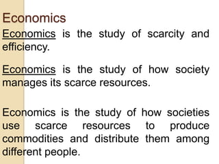


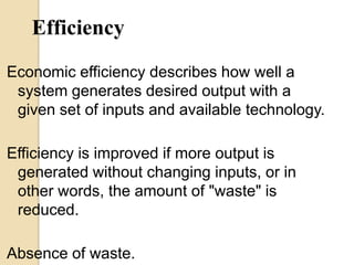


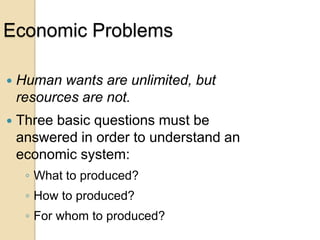


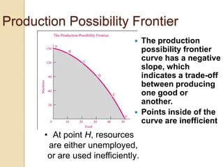
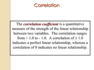
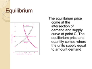
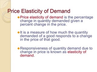
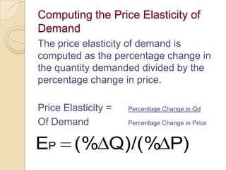
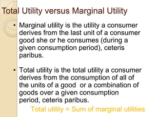
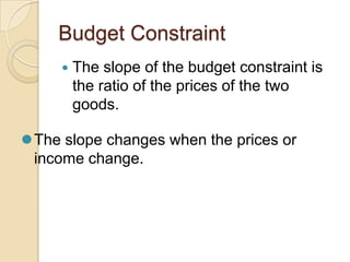
![An algebraic formula for correlation
coefficient
n
r
[ n(
2
x ) (
xy
x
2
x) ][ n(
y
2
y ) (
2
y) ]](https://image.slidesharecdn.com/economicschapter1-131204163010-phpapp01/85/Economics-chapter-1-53-320.jpg)

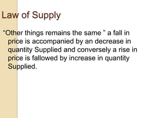


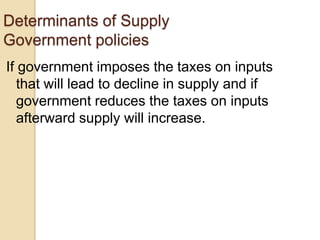
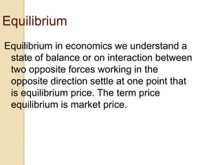
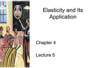
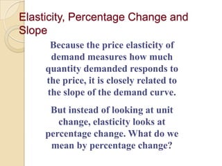


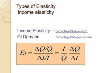


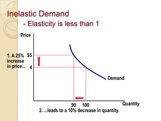

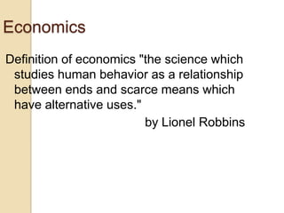
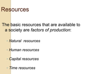
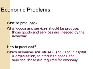
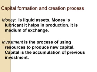
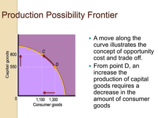
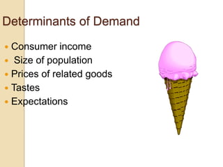
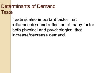
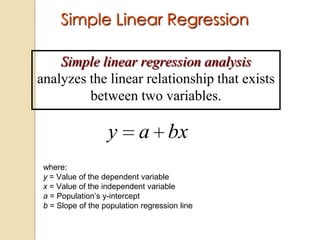
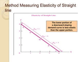
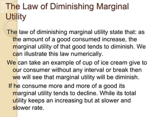
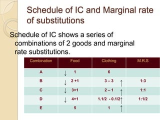
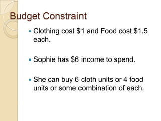
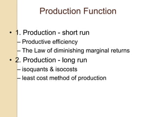
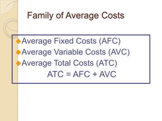
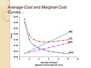
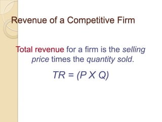
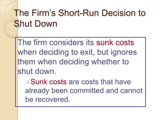
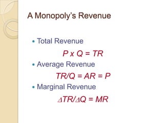
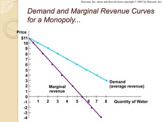
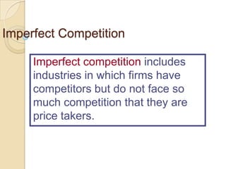
![Method Measuring Elasticity the
Average Formula
The Average (midpoint formula) is preferable when
calculating the price elasticity of demand because it
gives the same answer regardless of the direction of
the change.
(Q2 Q1 )/[(Q2 Q1 )/2]
Price Elasticity of Demand =
(P2 P1 )/[(P2 P1 )/2]](https://image.slidesharecdn.com/economicschapter1-131204163010-phpapp01/85/Economics-chapter-1-99-320.jpg)
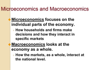
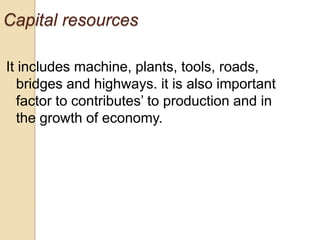
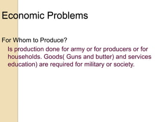
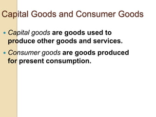
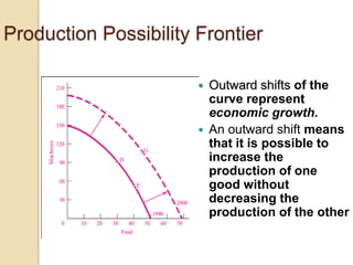
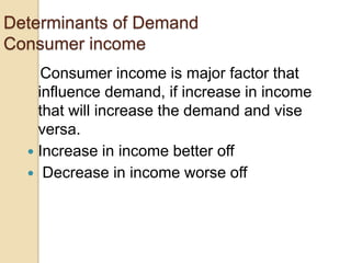
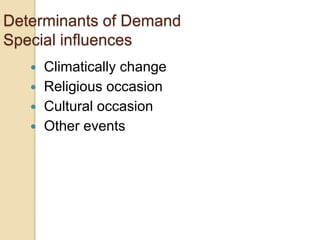
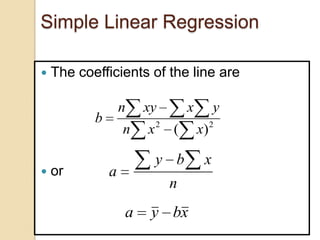
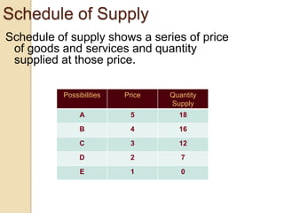
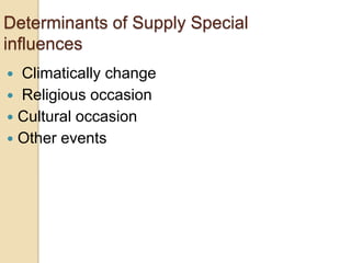
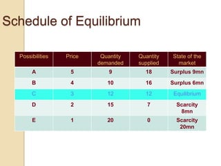
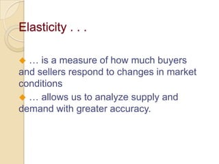
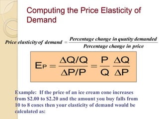
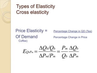
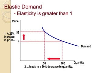
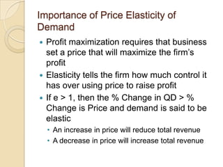
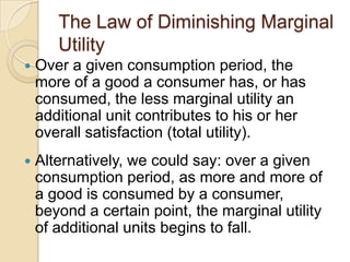
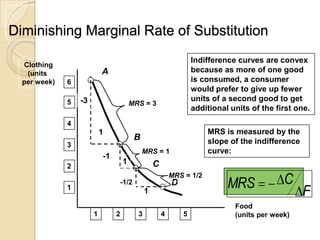
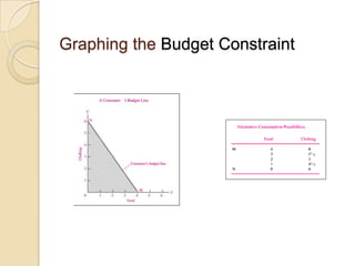
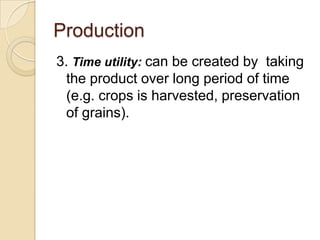
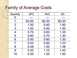
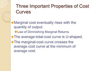
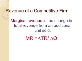
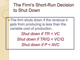
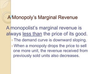
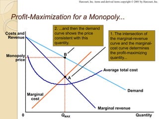
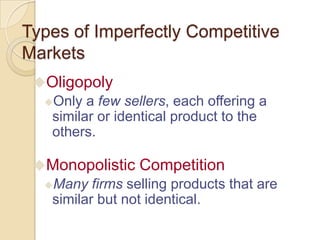
![Method Measuring Elasticity the
Average Formula
(Q 2 Q1 )/[(Q 2 Q1 )/2]
Price Elasticity of Demand =
(P2 P1 )/[(P2 P1 )/2]
Example: If the price of an ice cream cone increases
from $2.00 to $2.20 and the amount you buy falls from
10 to 8 cones the your elasticity of demand, using the
midpoint formula, would be calculated as:](https://image.slidesharecdn.com/economicschapter1-131204163010-phpapp01/85/Economics-chapter-1-100-320.jpg)

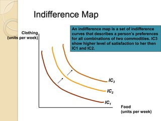


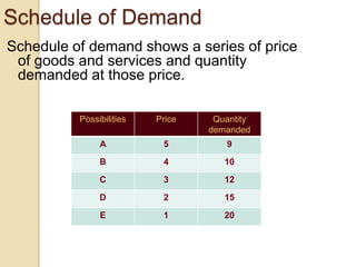
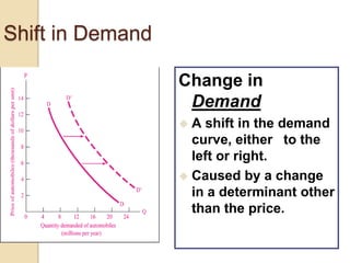
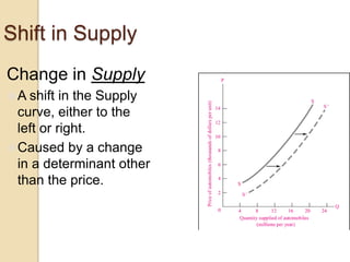
This document provides an overview of key economic concepts covered in chapters 1-3 of an economics textbook. It begins with definitions of economics and the founder of economics, Adam Smith. It then covers microeconomics and macroeconomics, scarcity, efficiency, factors of production, and the production possibility frontier. The document also discusses different economic systems, opportunity cost, demand and determinants of demand, the law of demand, supply and determinants of supply, and the law of supply.