Downloaded 775 times


![28
data once set via the initial construction of the object, in our interface. In other class designs
we might want to use setters, which are modifier methods used to set member data. It will all
depend upon the client requirements and how the code will fit into the grander scheme of other
objects.
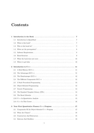
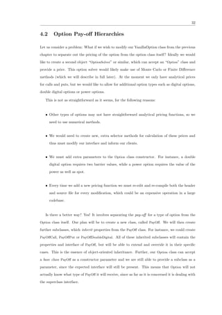
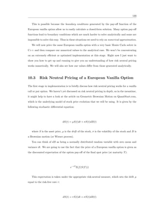
I will only display one method here (in this instance the retrieval of the strike price, K) as
the rest are extremely similar.
// Public access for the s t r i k e price , K
double VanillaOption : : getK () const { return K; }
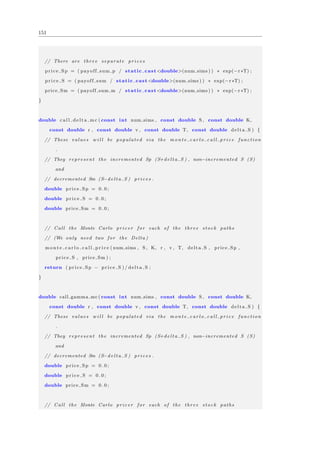
The final methods to implement are calc call price and calc put price . They are both public
and const. This forces them to be selector methods. This is what we want because a calculation
should not modify the underlying member data of the class instance. These methods produce
the analytical price of calls and puts based on the necessary five parameters.
The only undefined component of this method is the N(.) function. This is the cumulative
distribution function of the normal distribution. It has not been discussed here, but it is imple-
mented in the original header file for completeness. I have done this because I don’t think it
is instructive in aiding our object oriented example of a VanillaOption, rather it is a necessary
function for calculating the analytical price.
I won’t dwell on the specifics of the following formulae. They can be obtained from any
introductory quantitative analysis textbook. I would hope that you recognise them! If you
are unfamiliar with these functions, then I suggest taking a look at Joshi[12], Wilmott[26] or
Hull[10] to brush up on your derivatives pricing theory. The main issue for us is to study the
implementation.
double VanillaOption : : c a l c c a l l p r i c e () const {
double sigma sqrt T = sigma ∗ sqrt (T) ;
double d 1 = ( log (S/K) + ( r + sigma ∗ sigma ∗ 0.5 ) ∗ T ) / sigma sqrt T
;
double d 2 = d 1 − sigma sqrt T ;
return S ∗ N( d 1 ) − K ∗ exp(−r ∗T) ∗ N( d 2 ) ;
}
double VanillaOption : : c a l c p u t p r i c e () const {
double sigma sqrt T = sigma ∗ sqrt (T) ;
double d 1 = ( log (S/K) + ( r + sigma ∗ sigma ∗ 0.5 ) ∗ T ) / sigma sqrt T
;](https://image.slidesharecdn.com/266803730-cpp-quant-finance-ebook-20131003-180810164750/85/C-For-Quantitative-Finance-29-320.jpg)


![48
i f ( this == & rhs ) return ∗ this ; // Handling assignment to s e l f
mat = rhs . get mat () ;
return ∗ this ;
}
// Destructor
template <typename Type>
SimpleMatrix<Type >::˜ SimpleMatrix () {
// No need for implementation , as there i s no
// manual dynamic memory a l l o c a t i o n
}
// Matrix access method , via copying
template <typename Type>
SimpleMatrix<Type> SimpleMatrix<Type >:: get mat () const {
return mat ;
}
// Matrix access method , via row and column index
template <typename Type>
Type& SimpleMatrix<Type >:: value ( const int& row , const int& col ) {
return mat [ row ] [ col ] ;
}
#ENDIF
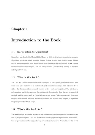
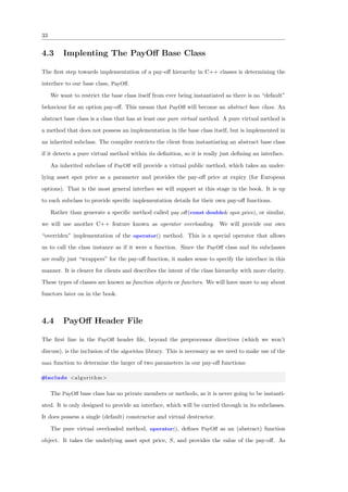
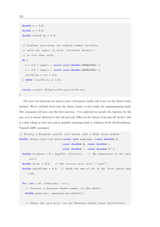
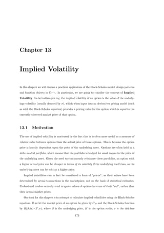
As with previous source files we are using pre-processor macros and have included the respec-
tive header file. We will begin by discussing the default constructor syntax:
// Default constructor
template <typename Type>
SimpleMatrix<Type >:: SimpleMatrix () {
// No need for implementation , as the vector ”mat”
// w i l l create the necessary storage
}
Beyond the comment, the first line states to the compiler that we are defining a function
template with a single typename, Type. The following line uses the scope resolution operator](https://image.slidesharecdn.com/266803730-cpp-quant-finance-ebook-20131003-180810164750/85/C-For-Quantitative-Finance-49-320.jpg)

![50
SimpleMatrix<Type>& SimpleMatrix<Type >:: operator=(const SimpleMatrix<Type>&
rhs )
{
i f ( this == & rhs ) return ∗ this ; // Handling assignment to s e l f
mat = rhs . get mat () ;
return ∗ this ;
}
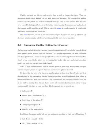
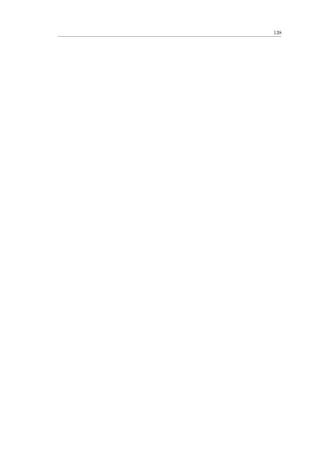
The assignment operator implementation is not too dissimilar to that of the copy constructor.
It basically states that if we try and assign the object to itself (i.e. my matrix = my matrix;) then
it should return a dereferenced pointer to this, the reference object to which the method is being
called on. If a non-self assignment occurs, then copy the matrix as in the copy constructor and
then return a dereferenced pointer to this.
The destructor does not have an implementation as there is no dynamic memory to deallocate:
// Destructor
template <typename Type>
SimpleMatrix<Type >::˜ SimpleMatrix () {
// No need for implementation , as there i s no
// manual dynamic memory a l l o c a t i o n
}
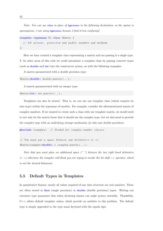
The last two public methods involve access to the underlying matrix data. get mat() returns
a copy of the matrix mat and, as stated above, is an inefficient method, but is still useful for
describing template syntax. Notice also that it is a const method, since it does not modify
anything:
// Matrix access method , via copying
template <typename Type>
SimpleMatrix<Type> SimpleMatrix<Type >:: get mat () const {
return mat ;
}
The final method, value (...) returns a direct reference to the underlying data type at a
particular row/column index. Hence it is not marked as const, because it is feasible (and
intended) that the data can be modified via this method. The method makes use of the []
operator, provided by the vector class in order to ease access to the underlying data:
// Matrix access method , via row and column index
template <typename Type>](https://image.slidesharecdn.com/266803730-cpp-quant-finance-ebook-20131003-180810164750/85/C-For-Quantitative-Finance-51-320.jpg)
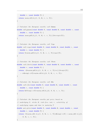
![51
Type& SimpleMatrix<Type >:: value ( const int& row , const int& col ) {
return mat [ row ] [ col ] ;
}
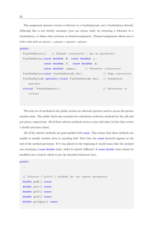
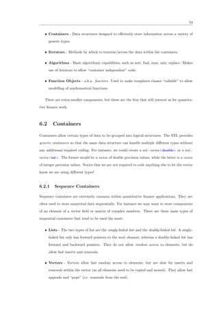
This completes the listing for the SimpleMatrix object. We will extend our matrix class in
later lessons to be far more efficient and useful.
5.8 Generic Programming vs OOP
One common question that arises when discussing templates is “Why use templates over normal
object orientation?”. Answers include:
• Generally more errors caught at compile time and less at run-time. Thus, there isn’t as
much need for try-catch exception blocks in your code.
• When using container classes with iteration. Modelling a Time Series or Binomial Lattice,
for instance. Generic programming offers a lot of flexibility here.
• The STL itself is dependent upon generic programming and so it is necessary to be familiar
with it.
However, templates themselves can lead to extremely cryptic compiler error messages, which
can take a substantial amount of time to debug. More often than not, these errors are due to
simple syntax errors. This is probably why generic programming has not been taken up as much
as the object oriented paradigm.](https://image.slidesharecdn.com/266803730-cpp-quant-finance-ebook-20131003-180810164750/85/C-For-Quantitative-Finance-52-320.jpg)


![57
• Input - An input iterator is a single-pass read-only iterator. In order to traverse elements,
the ++ increment operator is used. However, elements can only be read once. Input
iterators do not support the −− decrement operator, which is why they are termed single-
pass. Crucially, an input iterator is unable to modify elements. To access an element, the
∗ pointer dereference operator is utilised.
• Output - An output iterator is very similar to an input iterator with the major exception
that the iterator writes values instead of reading them. As with input iterators, writes can
only occur once and there is no means of stepping backwards. Also, it is only possible to
assign a value once to any individual element.
• Forward - A forward iterator is a combination of an input and output iterator. As before
the increment operator (++) allows forward stepping, but there is no decrement operator
support. To read or write to an element the pointer derefernce operator (∗) must be used.
However, unlike the previous two iterator categories, an element can be read or written to
multiple times.
• Bidirectional - A bidirectional iterator is similar to a forward iterator except that it
supports backward stepping via the decrement operator (−−).
• Random Access - A random access iterator is the most versatile iterator category and is
very much like a traditional C-style pointer. It possesses all the abilities of a bidirectional
iterator, with the addition of being able to access any index via the [] subscript operator.
Random access iterators also support pointer arithmetic so integer stepping is allowed.
Iterators are divided into these categories mainly for performance reasons. Certain iterators
are not supported with certain containers when C++ deems it likely that iteration will lead to
poor performance. For instance, random access iteration is not supported on the std :: list as
access to a random element would potentially require traversal of the entire linked-list used to
store the data. This is in contrast to a std :: vector where pointer arithmetic can be used to step
directly to the desired item.
6.3.2 Iterator Adaptors
Iterator adaptors allow iterators to be modified to allow special functionality. In particular,
iterators can be reversed, they can be modified to insert rather than overwrite and can be
adapted to work with streams.](https://image.slidesharecdn.com/266803730-cpp-quant-finance-ebook-20131003-180810164750/85/C-For-Quantitative-Finance-58-320.jpg)


![82
matrix with. Since the “vector of vectors” constructor has already been called at this stage, we
need to call its resize method in order to have enough elements to act as the row containers. Once
the matrix mat has been resized, we need to resize each individual vector within the rows to the
length representing the number of columns. The resize method can take an optional argument,
which will initialise all elements to that particular value. Finally we adjust the private rows and
cols unsigned integers to store the new row and column counts:
// Parameter Constructor
template<typename T>
QSMatrix<T>:: QSMatrix (unsigned rows , unsigned col s , const T& i n i t i a l ) {
mat . r e s i z e ( rows ) ;
for ( unsigned i =0; i<mat . s i z e () ; i++) {
mat [ i ] . r e s i z e ( col s , i n i t i a l ) ;
}
rows = rows ;
c o l s = c o l s ;
}
The copy constructor has a straightforward implementation. Since we have not used any
dynamic memory allocation, we simply need to copy each private member from the corresponding
copy matrix rhs:
// Copy Constructor
template<typename T>
QSMatrix<T>:: QSMatrix ( const QSMatrix<T>& rhs ) {
mat = rhs . mat ;
rows = rhs . get rows () ;
c o l s = rhs . g e t c o l s () ;
}
The destructor is even simpler. Since there is no dynamic memory allocation, we don’t need
to do anything. We can let the compiler handle the destruction of the individual type members
(mat, rows and cols):
// ( Virtual ) Destructor
template<typename T>
QSMatrix<T>::˜ QSMatrix () {}
The assignment operator is somewhat more complicated than the other construction/destruc-
tion methods. The first two lines of the method implementation check that the addresses of the](https://image.slidesharecdn.com/266803730-cpp-quant-finance-ebook-20131003-180810164750/85/C-For-Quantitative-Finance-83-320.jpg)
![83
two matrices aren’t identical (i.e. we’re not trying to assign a matrix to itself). If this is the
case, then just return the dereferenced pointer to the current object (∗this). This is purely for
performance reasons. Why go through the process of copying exactly the same data into itself if
it is already identical?
However, if the matrix in-memory addresses differ, then we resize the old matrix to the be
the same size as the rhs matrix. Once that is complete we then populate the values element-
wise and finally adjust the members holding the number of rows and columns. We then return
the dereferenced pointer to this. This is a common pattern for assignment operators and is
considered good practice:
// Assignment Operator
template<typename T>
QSMatrix<T>& QSMatrix<T>:: operator=(const QSMatrix<T>& rhs ) {
i f (&rhs == this )
return ∗ this ;
unsigned new rows = rhs . get rows () ;
unsigned new cols = rhs . g e t c o l s () ;
mat . r e s i z e ( new rows ) ;
for ( unsigned i =0; i<mat . s i z e () ; i++) {
mat [ i ] . r e s i z e ( new cols ) ;
}
for ( unsigned i =0; i<new rows ; i++) {
for ( unsigned j =0; j<new cols ; j++) {
mat [ i ] [ j ] = rhs ( i , j ) ;
}
}
rows = new rows ;
c o l s = new cols ;
return ∗ this ;
}](https://image.slidesharecdn.com/266803730-cpp-quant-finance-ebook-20131003-180810164750/85/C-For-Quantitative-Finance-84-320.jpg)
![84
8.1.6 Mathematical Operators Implementation
The next part of the implementation concerns the methods overloading the binary operators
that allow matrix algebra such as addition, subtraction and multiplication. There are two types
of operators to be overloaded here. The first is operation without assignment. The second is
operation with assignment. The first type of operator method creates a new matrix to store the
result of an operation (such as addition), while the second type applies the result of the operation
into the left-hand argument. For instance the first type will produce a new matrix C, from the
equation C = A + B. The second type will overwrite A with the result of A + B.
The first operator to implement is for addition without assignment. A new matrix result is
created with initial filled values equal to 0. Then each element is iterated through to be the
pairwise sum of the this matrix and the new right hand side matrix rhs. Notice that we use the
pointer dereferencing syntax with this when accessing the element values: this−>mat[i][j]. This
is identical to writing (∗this).mat[i ][ j ]. We must dereference the pointer before we can access
the underlying object. Finally, we return the result:
Note that this can be a particularly expensive operation. We are creating a new matrix for
every call of this method. However, modern compilers are smart enough to make sure that this
operation is not as performance heavy as it used to be, so for our current needs we are justified
in creating the matrix here. Note again that if we were to return a matrix by reference and then
create the matrix within the class via the new operator, we would have an error as the matrix
object would go out of scope as soon as the method returned.
// Addition of two matrices
template<typename T>
QSMatrix<T> QSMatrix<T>:: operator+(const QSMatrix<T>& rhs ) {
QSMatrix r e s u l t ( rows , cols , 0 .0 ) ;
for ( unsigned i =0; i<rows ; i++) {
for ( unsigned j =0; j<c o l s ; j++) {
r e s u l t ( i , j ) = this−>mat [ i ] [ j ] + rhs ( i , j ) ;
}
}
return r e s u l t ;
}
The operation with assignment method for addition is carried out slightly differently. It](https://image.slidesharecdn.com/266803730-cpp-quant-finance-ebook-20131003-180810164750/85/C-For-Quantitative-Finance-85-320.jpg)
![85
DOES return a reference to an object, but this is fine since the object reference it returns is
to this, which exists outside of the scope of the method. The method itself makes use of the
operator+= that is bound to the type object. Thus when we carry out the line this−>mat
[i][j] += rhs(i,j); we are making use of the types own operator overload. Finally, we return a
dereferenced pointer to this giving us back the modified matrix:
// Cumulative addition of t h i s matrix and another
template<typename T>
QSMatrix<T>& QSMatrix<T>:: operator+=(const QSMatrix<T>& rhs ) {
unsigned rows = rhs . get rows () ;
unsigned c o l s = rhs . g e t c o l s () ;
for ( unsigned i =0; i<rows ; i++) {
for ( unsigned j =0; j<c o l s ; j++) {
this−>mat [ i ] [ j ] += rhs ( i , j ) ;
}
}
return ∗ this ;
}
The two matrix subtraction operators operator− and operator−= are almost identical to
the addition variants, so I won’t explain them here. If you wish to see their implementation,
have a look at the full listing below.
I will discuss the matrix multiplication methods though as their syntax is sufficiently different
to warrant explanation. The first operator is that without assignment, operator∗. We can use
this to carry out an equation of the form C = A × B. The first part of the method creates a
new result matrix that has the same size as the right hand side matrix, rhs. Then we perform
the triple loop associated with matrix multiplication. We iterate over each element in the result
matrix and assign it the value of this−>mat[i][k] ∗ rhs(k,j), i.e. the value of Aik × Bkj, for
k ∈ {0, ..., M − 1}:
// Left m u l t i p l i c a t i o n of t h i s matrix and another
template<typename T>
QSMatrix<T> QSMatrix<T>:: operator ∗( const QSMatrix<T>& rhs ) {
unsigned rows = rhs . get rows () ;
unsigned c o l s = rhs . g e t c o l s () ;
QSMatrix r e s u l t ( rows , cols , 0 .0 ) ;](https://image.slidesharecdn.com/266803730-cpp-quant-finance-ebook-20131003-180810164750/85/C-For-Quantitative-Finance-86-320.jpg)
![86
for ( unsigned i =0; i<rows ; i++) {
for ( unsigned j =0; j<c o l s ; j++) {
for ( unsigned k=0; k<rows ; k++) {
r e s u l t ( i , j ) += this−>mat [ i ] [ k ] ∗ rhs (k , j ) ;
}
}
}
return r e s u l t ;
}
The implementation of the operator∗= is far simpler, but only because we are building on
what already exists. The first line creates a new matrix called result which stores the result of
multiplying the dereferenced pointer to this and the right hand side matrix, rhs. The second line
then sets this to be equal to the result above. This is necessary as if it was carried out in one
step, data would be overwritten before it could be used, creating an incorrect result. Finally the
referenced pointer to this is returned. Most of the work is carried out by the operator∗ which
is defined above. The listing is as follows:
// Cumulative l e f t m u l t i p l i c a t i o n of t h i s matrix and another
template<typename T>
QSMatrix<T>& QSMatrix<T>:: operator∗=(const QSMatrix<T>& rhs ) {
QSMatrix r e s u l t = (∗ this ) ∗ rhs ;
(∗ this ) = r e s u l t ;
return ∗ this ;
}
We also wish to apply scalar element-wise operations to the matrix, in particular element-wise
scalar addition, subtraction, multiplication and division. Since they are all very similar, I will
only provide explanation for the addition operator. The first point of note is that the parameter
is now a const T&, i.e. a reference to a const type. This is the scalar value that will be added
to all matrix elements. We then create a new result matrix as before, of identical size to this.
Then we iterate over the elements of the result matrix and set their values equal to the sum of
the individual elements of this and our type value, rhs. Finally, we return the result matrix:
// Matrix/ s c a l a r addition
template<typename T>](https://image.slidesharecdn.com/266803730-cpp-quant-finance-ebook-20131003-180810164750/85/C-For-Quantitative-Finance-87-320.jpg)
![87
QSMatrix<T> QSMatrix<T>:: operator+(const T& rhs ) {
QSMatrix r e s u l t ( rows , cols , 0 .0 ) ;
for ( unsigned i =0; i<rows ; i++) {
for ( unsigned j =0; j<c o l s ; j++) {
r e s u l t ( i , j ) = this−>mat [ i ] [ j ] + rhs ;
}
}
return r e s u l t ;
}
We also wish to allow (right) matrix vector multiplication. It is not too different from the
implementation of matrix-matrix multiplication. In this instance we are returning a std :: vector
<T> and also providing a separate vector as a parameter. Upon invocation of the method we
create a new result vector that has the same size as the right hand side, rhs. Then we perform
a double loop over the elements of the this matrix and assign the result to an element of the
result vector. Finally, we return the result vector:
// Multiply a matrix with a vector
template<typename T>
std : : vector<T> QSMatrix<T>:: operator ∗( const std : : vector<T>& rhs ) {
std : : vector<T> r e s u l t ( rhs . s i z e () , 0 .0 ) ;
for ( unsigned i =0; i<rows ; i++) {
for ( unsigned j =0; j<c o l s ; j++) {
r e s u l t [ i ] = this−>mat [ i ] [ j ] ∗ rhs [ j ] ;
}
}
return r e s u l t ;
}
I’ve added a final matrix method, which is useful for certain numerical linear algebra tech-
niques. Essentially it returns a vector of the diagonal elements of the matrix. Firstly we create
the result vector, then assign it the values of the diagonal elements and finally we return the
result vector:
// Obtain a vector of the diagonal elements](https://image.slidesharecdn.com/266803730-cpp-quant-finance-ebook-20131003-180810164750/85/C-For-Quantitative-Finance-88-320.jpg)
![88
template<typename T>
std : : vector<T> QSMatrix<T>:: diag vec () {
std : : vector<T> r e s u l t ( rows , 0 . 0 ) ;
for ( unsigned i =0; i<rows ; i++) {
r e s u l t [ i ] = this−>mat [ i ] [ i ] ;
}
return r e s u l t ;
}
The final set of methods to implement are for accessing the individual elements as well as
getting the number of rows and columns from the matrix. They’re all quite simple in their
implementation. They dereference this and then obtain either an individual element or some
private member data:
// Access the i n d i v i d u a l elements
template<typename T>
T& QSMatrix<T>:: operator () ( const unsigned& row , const unsigned& col ) {
return this−>mat [ row ] [ col ] ;
}
// Access the i n d i v i d u a l elements ( const )
template<typename T>
const T& QSMatrix<T>:: operator () ( const unsigned& row , const unsigned& col )
const {
return this−>mat [ row ] [ col ] ;
}
// Get the number of rows of the matrix
template<typename T>
unsigned QSMatrix<T>:: get rows () const {
return this−>rows ;
}
// Get the number of columns of the matrix
template<typename T>
unsigned QSMatrix<T>:: g e t c o l s () const {](https://image.slidesharecdn.com/266803730-cpp-quant-finance-ebook-20131003-180810164750/85/C-For-Quantitative-Finance-89-320.jpg)
![89
return this−>c o l s ;
}
8.1.7 Full Source Implementation
Now that we have described all the methods in full, here is the full source listing for the QSMatrix
class:
#ifndef QS MATRIX CPP
#define QS MATRIX CPP
#include ” matrix . h”
// Parameter Constructor
template<typename T>
QSMatrix<T>:: QSMatrix (unsigned rows , unsigned col s , const T& i n i t i a l ) {
mat . r e s i z e ( rows ) ;
for ( unsigned i =0; i<mat . s i z e () ; i++) {
mat [ i ] . r e s i z e ( col s , i n i t i a l ) ;
}
rows = rows ;
c o l s = c o l s ;
}
// Copy Constructor
template<typename T>
QSMatrix<T>:: QSMatrix ( const QSMatrix<T>& rhs ) {
mat = rhs . mat ;
rows = rhs . get rows () ;
c o l s = rhs . g e t c o l s () ;
}
// ( Virtual ) Destructor
template<typename T>
QSMatrix<T>::˜ QSMatrix () {}
// Assignment Operator
template<typename T>](https://image.slidesharecdn.com/266803730-cpp-quant-finance-ebook-20131003-180810164750/85/C-For-Quantitative-Finance-90-320.jpg)
![90
QSMatrix<T>& QSMatrix<T>:: operator=(const QSMatrix<T>& rhs ) {
i f (&rhs == this )
return ∗ this ;
unsigned new rows = rhs . get rows () ;
unsigned new cols = rhs . g e t c o l s () ;
mat . r e s i z e ( new rows ) ;
for ( unsigned i =0; i<mat . s i z e () ; i++) {
mat [ i ] . r e s i z e ( new cols ) ;
}
for ( unsigned i =0; i<new rows ; i++) {
for ( unsigned j =0; j<new cols ; j++) {
mat [ i ] [ j ] = rhs ( i , j ) ;
}
}
rows = new rows ;
c o l s = new cols ;
return ∗ this ;
}
// Addition of two matrices
template<typename T>
QSMatrix<T> QSMatrix<T>:: operator+(const QSMatrix<T>& rhs ) {
QSMatrix r e s u l t ( rows , cols , 0 .0 ) ;
for ( unsigned i =0; i<rows ; i++) {
for ( unsigned j =0; j<c o l s ; j++) {
r e s u l t ( i , j ) = this−>mat [ i ] [ j ] + rhs ( i , j ) ;
}
}
return r e s u l t ;
}](https://image.slidesharecdn.com/266803730-cpp-quant-finance-ebook-20131003-180810164750/85/C-For-Quantitative-Finance-91-320.jpg)
![91
// Cumulative addition of t h i s matrix and another
template<typename T>
QSMatrix<T>& QSMatrix<T>:: operator+=(const QSMatrix<T>& rhs ) {
unsigned rows = rhs . get rows () ;
unsigned c o l s = rhs . g e t c o l s () ;
for ( unsigned i =0; i<rows ; i++) {
for ( unsigned j =0; j<c o l s ; j++) {
this−>mat [ i ] [ j ] += rhs ( i , j ) ;
}
}
return ∗ this ;
}
// Subtraction of t h i s matrix and another
template<typename T>
QSMatrix<T> QSMatrix<T>:: operator−(const QSMatrix<T>& rhs ) {
unsigned rows = rhs . get rows () ;
unsigned c o l s = rhs . g e t c o l s () ;
QSMatrix r e s u l t ( rows , cols , 0 .0 ) ;
for ( unsigned i =0; i<rows ; i++) {
for ( unsigned j =0; j<c o l s ; j++) {
r e s u l t ( i , j ) = this−>mat [ i ] [ j ] − rhs ( i , j ) ;
}
}
return r e s u l t ;
}
// Cumulative s u b t r a c t i o n of t h i s matrix and another
template<typename T>
QSMatrix<T>& QSMatrix<T>:: operator−=(const QSMatrix<T>& rhs ) {
unsigned rows = rhs . get rows () ;
unsigned c o l s = rhs . g e t c o l s () ;](https://image.slidesharecdn.com/266803730-cpp-quant-finance-ebook-20131003-180810164750/85/C-For-Quantitative-Finance-92-320.jpg)
![92
for ( unsigned i =0; i<rows ; i++) {
for ( unsigned j =0; j<c o l s ; j++) {
this−>mat [ i ] [ j ] −= rhs ( i , j ) ;
}
}
return ∗ this ;
}
// Left m u l t i p l i c a t i o n of t h i s matrix and another
template<typename T>
QSMatrix<T> QSMatrix<T>:: operator ∗( const QSMatrix<T>& rhs ) {
unsigned rows = rhs . get rows () ;
unsigned c o l s = rhs . g e t c o l s () ;
QSMatrix r e s u l t ( rows , cols , 0 .0 ) ;
for ( unsigned i =0; i<rows ; i++) {
for ( unsigned j =0; j<c o l s ; j++) {
for ( unsigned k=0; k<rows ; k++) {
r e s u l t ( i , j ) += this−>mat [ i ] [ k ] ∗ rhs (k , j ) ;
}
}
}
return r e s u l t ;
}
// Cumulative l e f t m u l t i p l i c a t i o n of t h i s matrix and another
template<typename T>
QSMatrix<T>& QSMatrix<T>:: operator∗=(const QSMatrix<T>& rhs ) {
QSMatrix r e s u l t = (∗ this ) ∗ rhs ;
(∗ this ) = r e s u l t ;
return ∗ this ;
}
// Calculate a transpose of t h i s matrix
template<typename T>](https://image.slidesharecdn.com/266803730-cpp-quant-finance-ebook-20131003-180810164750/85/C-For-Quantitative-Finance-93-320.jpg)
![93
QSMatrix<T> QSMatrix<T>:: transpose () {
QSMatrix r e s u l t ( rows , cols , 0 .0 ) ;
for ( unsigned i =0; i<rows ; i++) {
for ( unsigned j =0; j<c o l s ; j++) {
r e s u l t ( i , j ) = this−>mat [ j ] [ i ] ;
}
}
return r e s u l t ;
}
// Matrix/ s c a l a r addition
template<typename T>
QSMatrix<T> QSMatrix<T>:: operator+(const T& rhs ) {
QSMatrix r e s u l t ( rows , cols , 0 .0 ) ;
for ( unsigned i =0; i<rows ; i++) {
for ( unsigned j =0; j<c o l s ; j++) {
r e s u l t ( i , j ) = this−>mat [ i ] [ j ] + rhs ;
}
}
return r e s u l t ;
}
// Matrix/ s c a l a r s u b tr a c t i o n
template<typename T>
QSMatrix<T> QSMatrix<T>:: operator−(const T& rhs ) {
QSMatrix r e s u l t ( rows , cols , 0 .0 ) ;
for ( unsigned i =0; i<rows ; i++) {
for ( unsigned j =0; j<c o l s ; j++) {
r e s u l t ( i , j ) = this−>mat [ i ] [ j ] − rhs ;
}
}](https://image.slidesharecdn.com/266803730-cpp-quant-finance-ebook-20131003-180810164750/85/C-For-Quantitative-Finance-94-320.jpg)
![94
return r e s u l t ;
}
// Matrix/ s c a l a r m u l t i p l i c a t i o n
template<typename T>
QSMatrix<T> QSMatrix<T>:: operator ∗( const T& rhs ) {
QSMatrix r e s u l t ( rows , cols , 0 .0 ) ;
for ( unsigned i =0; i<rows ; i++) {
for ( unsigned j =0; j<c o l s ; j++) {
r e s u l t ( i , j ) = this−>mat [ i ] [ j ] ∗ rhs ;
}
}
return r e s u l t ;
}
// Matrix/ s c a l a r d i v i s i o n
template<typename T>
QSMatrix<T> QSMatrix<T>:: operator /( const T& rhs ) {
QSMatrix r e s u l t ( rows , cols , 0 .0 ) ;
for ( unsigned i =0; i<rows ; i++) {
for ( unsigned j =0; j<c o l s ; j++) {
r e s u l t ( i , j ) = this−>mat [ i ] [ j ] / rhs ;
}
}
return r e s u l t ;
}
// Multiply a matrix with a vector
template<typename T>
std : : vector<T> QSMatrix<T>:: operator ∗( const std : : vector<T>& rhs ) {
std : : vector<T> r e s u l t ( rhs . s i z e () , 0 .0 ) ;
for ( unsigned i =0; i<rows ; i++) {](https://image.slidesharecdn.com/266803730-cpp-quant-finance-ebook-20131003-180810164750/85/C-For-Quantitative-Finance-95-320.jpg)
![95
for ( unsigned j =0; j<c o l s ; j++) {
r e s u l t [ i ] = this−>mat [ i ] [ j ] ∗ rhs [ j ] ;
}
}
return r e s u l t ;
}
// Obtain a vector of the diagonal elements
template<typename T>
std : : vector<T> QSMatrix<T>:: diag vec () {
std : : vector<T> r e s u l t ( rows , 0 . 0 ) ;
for ( unsigned i =0; i<rows ; i++) {
r e s u l t [ i ] = this−>mat [ i ] [ i ] ;
}
return r e s u l t ;
}
// Access the i n d i v i d u a l elements
template<typename T>
T& QSMatrix<T>:: operator () ( const unsigned& row , const unsigned& col ) {
return this−>mat [ row ] [ col ] ;
}
// Access the i n d i v i d u a l elements ( const )
template<typename T>
const T& QSMatrix<T>:: operator () ( const unsigned& row , const unsigned& col )
const {
return this−>mat [ row ] [ col ] ;
}
// Get the number of rows of the matrix
template<typename T>
unsigned QSMatrix<T>:: get rows () const {
return this−>rows ;](https://image.slidesharecdn.com/266803730-cpp-quant-finance-ebook-20131003-180810164750/85/C-For-Quantitative-Finance-96-320.jpg)


![99
4 , 5 , 6 ,
7 , 8 , 9;
std : : cout << m << std : : endl ;
}
Here is the (rather simple!) output for the above program:
1 2 3
4 5 6
7 8 9
Notice that the overloaded << operator can accept comma-separated lists of values in order
to initialise the matrix. This is an extremely useful part of the API syntax. In addition, we can
also pass the MatrixXd to std :: cout and have the numbers output in a human-readable fashion.
8.2.3 Basic Linear Algebra
Eigen is a large library and has many features. We will be exploring many of them over subsequent
chapters. In this section I want to describe basic matrix and vector operations, including the
matrix-vector and matrix-matrix multiplication facilities provided with the library.
8.2.4 Expression Templates
One of the most attractive features of the Eigen library is that it includes expression objects and
lazy evaluation. This means that any arithmetic operation actually returns such an expression
object, which is actually a description of the final computation to be performed rather than
the actual computation itself. The benefit of such an approach is that most compilers are able
to heavily optimise the expression such that additional loops are completely minimised. As an
example, an expression such as:
VectorXd p (10) , q (10) , r (10) , s (10) ;
. . .
p = 5∗q + 11∗ r − 7∗ s ;
will compile into a single loop:
for (unsigned i =0; i <10; ++i ) {
p [ i ] = 5∗q [ i ] + 11∗ r [ i ] − 7∗ s [ i ] ;
}
This means that the underlying storage arrays are only looped over once. As such Eigen can
optimise relatively complicated arithmetic expressions.](https://image.slidesharecdn.com/266803730-cpp-quant-finance-ebook-20131003-180810164750/85/C-For-Quantitative-Finance-100-320.jpg)


![112
1 c∗
1 0 0 ... 0
0 1 c∗
2 0 ... 0
0 0 1 c∗
3 0 0
. . .
. . .
. . c∗
k−1
0 0 0 0 0 1
f1
f2
f3
.
.
.
fk
=
d∗
1
d∗
2
d∗
3
.
.
.
d∗
k
The algorithm for the solution of these equations is now straightforward and works ’in reverse’:
fk = d∗
k, fi = d∗
k − c∗
i xi+1, i = k − 1, k − 2, ..., 2, 1
9.3.1 C++ Implementation
You can see the function prototype here:
void thomas algorithm ( const std : : vector<double>& a ,
const std : : vector<double>& b ,
const std : : vector<double>& c ,
const std : : vector<double>& d ,
std : : vector<double>& f ) {
Notice that f is a non-const vector, which means it is the only vector to be modified within
the function.
It is possible to write the Thomas Algorithm function in a more efficient manner to override
the c and d vectors. Finite difference methods require the vectors to be re-used for each time
step, so the following implementation utilises two additional temporary vectors, c∗
and d∗
. The
memory for the vectors has been allocated within the function. Every time the function is called
these vectors are allocated and deallocated, which is suboptimal from an efficiency point of view.
A proper ”production” implementation would pass references to these vectors from an exter-
nal function that only requires a single allocation and deallocation. However, in order to keep
the function straightforward to understand I’ve not included this aspect:
std : : vector<double> c s t a r (N, 0 .0 ) ;
std : : vector<double> d star (N, 0. 0 ) ;
The first step in the algorithm is to initialise the beginning elements of the c∗
and d∗
vectors:
c s t a r [ 0 ] = c [ 0 ] / b [ 0 ] ;](https://image.slidesharecdn.com/266803730-cpp-quant-finance-ebook-20131003-180810164750/85/C-For-Quantitative-Finance-113-320.jpg)
![113
d star [ 0 ] = d [ 0 ] / b [ 0 ] ;
The next step, known as the ”forward sweep” is to fill the c∗
and d∗
vectors such that we
form the second matrix equation A∗
f = d∗
:
for ( int i =1; i<N; i++) {
double m = 1.0 / (b [ i ] − a [ i ] ∗ c s t a r [ i −1]) ;
c s t a r [ i ] = c [ i ] ∗ m;
d star [ i ] = (d [ i ] − a [ i ] ∗ d star [ i −1]) ∗ m;
}
Once the forward sweep is carried out the final step is to carry out the ”reverse sweep”.
Notice that the vector f is actually being assigned here. The function itself is void, so we don’t
return any values.
for ( int i=N−1; i−− > 0; ) {
f [ i ] = d star [ i ] − c s t a r [ i ] ∗ d [ i +1];
}
I’ve included a main function, which sets up the Thomas Algorithm to solve one time-step
of the Crank-Nicolson finite difference method discretised diffusion equation. The details of the
algorithm are not so important here, as I will be elucidating on the method in further articles
on QuantStart.com when we come to solve the Black-Scholes equation. This is only provided in
order to show you how the function works in a ”real world” situation:
#include <cmath>
#include <iostream>
#include <vector>
// Vectors a , b , c and d are const . They w i l l not be modified
// by the function . Vector f ( the s o l u t i o n vector ) i s non−const
// and thus w i l l be c a l c u l a t e d and updated by the function .
void thomas algorithm ( const std : : vector<double>& a ,
const std : : vector<double>& b ,
const std : : vector<double>& c ,
const std : : vector<double>& d ,
std : : vector<double>& f ) {
s i z e t N = d . s i z e () ;
// Create the temporary vectors](https://image.slidesharecdn.com/266803730-cpp-quant-finance-ebook-20131003-180810164750/85/C-For-Quantitative-Finance-114-320.jpg)
![114
// Note that t h i s i s i n e f f i c i e n t as i t i s p o s s i b l e to c a l l
// t h i s function many times . A b e t t e r implementation would
// pass these temporary matrices by non−const reference to
// save excess a l l o c a t i o n and d e a l l o c a t i o n
std : : vector<double> c s t a r (N, 0 .0 ) ;
std : : vector<double> d star (N, 0. 0 ) ;
// This updates the c o e f f i c i e n t s in the f i r s t row
// Note that we should be checking for d i v i s i o n by zero here
c s t a r [ 0 ] = c [ 0 ] / b [ 0 ] ;
d star [ 0 ] = d [ 0 ] / b [ 0 ] ;
// Create the c s t a r and d s t a r c o e f f i c i e n t s in the forward sweep
for ( int i =1; i<N; i++) {
double m = 1.0 / (b [ i ] − a [ i ] ∗ c s t a r [ i −1]) ;
c s t a r [ i ] = c [ i ] ∗ m;
d star [ i ] = (d [ i ] − a [ i ] ∗ d star [ i −1]) ∗ m;
}
// This i s the reverse sweep , used to update the s o l u t i o n vector f
for ( int i=N−1; i−− > 0; ) {
f [ i ] = d star [ i ] − c s t a r [ i ] ∗ d [ i +1];
}
}
// Although thomas algorithm provides everything necessary to s o l v e
// a t r i d i a g o n a l system , i t i s h e l p f u l to wrap i t up in a ” r e a l world ”
// example . The main function below uses a t r i d i a g o n a l system from
// a Boundary Value Problem (BVP) . This i s the d i s c r e t i s a t i o n of the
// 1D heat equation .
int main ( int argc , char ∗∗ argv ) {
// Create a Finite Difference Method (FDM) mesh with 13 points
// using the Crank−Nicolson method to s o l v e the d i s c r e t i s e d
// heat equation .
s i z e t N = 13;
double delta x = 1.0/ static cast<double>(N) ;](https://image.slidesharecdn.com/266803730-cpp-quant-finance-ebook-20131003-180810164750/85/C-For-Quantitative-Finance-115-320.jpg)
![115
double d e l t a t = 0 . 0 0 1 ;
double r = d e l t a t /( delta x ∗ delta x ) ;
// F i rs t we create the vectors to store the c o e f f i c i e n t s
std : : vector<double> a (N−1, −r /2.0) ;
std : : vector<double> b(N, 1.0+ r ) ;
std : : vector<double> c (N−1, −r /2.0) ;
std : : vector<double> d(N, 0 . 0 ) ;
std : : vector<double> f (N, 0 .0 ) ;
// F i l l in the current time step i n i t i a l value
// vector using three peaks with various amplitudes
f [ 5 ] = 1; f [ 6 ] = 2; f [ 7 ] = 1;
// We output the s o l u t i o n vector f , prior to a
// new time−step
std : : cout << ” f = ( ” ;
for ( int i =0; i<N; i++) {
std : : cout << f [ i ] ;
i f ( i < N−1) {
std : : cout << ” , ” ;
}
}
std : : cout << ” ) ” << std : : endl << std : : endl ;
// F i l l in the current time step vector d
for ( int i =1; i<N−1; i++) {
d [ i ] = r ∗0.5∗ f [ i +1] + (1.0 − r ) ∗ f [ i ] + r ∗0.5∗ f [ i −1];
}
// Now we s o l v e the t r i d i a g o n a l system
thomas algorithm (a , b , c , d , f ) ;
// F i n al l y we output the s o l u t i o n vector f
std : : cout << ” f = ( ” ;
for ( int i =0; i<N; i++) {
std : : cout << f [ i ] ;](https://image.slidesharecdn.com/266803730-cpp-quant-finance-ebook-20131003-180810164750/85/C-For-Quantitative-Finance-116-320.jpg)


![162
#include <vector>
#include <cmath>
// For random Gaussian generation
// Note that there are many ways of doing this , but we w i l l
// be using the Box−Muller method for demonstration purposes
double gaussian box muller () {
double x = 0 . 0 ;
double y = 0 . 0 ;
double e u c l i d s q = 0 . 0 ;
do {
x = 2.0 ∗ rand () / static cast<double>(RANDMAX) −1;
y = 2.0 ∗ rand () / static cast<double>(RANDMAX) −1;
e u c l i d s q = x∗x + y∗y ;
} while ( e u c l i d s q >= 1 .0 ) ;
return x∗ sqrt (−2∗ log ( e u c l i d s q ) / e u c l i d s q ) ;
}
// This provides a vector containing sampled points of a
// Geometric Brownian Motion stock price path
void c a l c p a t h s p o t p r i c e s ( std : : vector<double>& spot prices , // Asset path
const double& r , // Risk f r e e i n t e r e s t rate
const double& v , // V o l a t i l i t y of underlying
const double& T) { // Expiry
// Since the d r i f t and v o l a t i l i t y of the a s s e t are constant
// we w i l l p r e c a l c u l a t e as much as p o s s i b l e for maximum e f f i c i e n c y
double dt = T/ static cast<double>( s p o t p r i c e s . s i z e () ) ;
double d r i f t = exp ( dt ∗( r −0.5∗v∗v) ) ;
double vol = sqrt (v∗v∗dt ) ;
for ( int i =1; i<s p o t p r i c e s . s i z e () ; i++) {
double gauss bm = gaussian box muller () ;
s p o t p r i c e s [ i ] = s p o t p r i c e s [ i −1] ∗ d r i f t ∗ exp ( vol ∗gauss bm ) ;
}](https://image.slidesharecdn.com/266803730-cpp-quant-finance-ebook-20131003-180810164750/85/C-For-Quantitative-Finance-163-320.jpg)
![163
}
#endif
Turning our attention to calc path spot prices we can see that the function requires a vector
of doubles, the risk-free rate r, the volatility of the underlying σ and the time at expiry, T:
void c a l c p a t h s p o t p r i c e s ( std : : vector<double>& spot prices , // Asset path
const double& r , // Risk f r e e i n t e r e s t rate (
constant )
const double& v , // V o l a t i l i t y of underlying (
constant )
const double& T) { // Expiry
Since we are dealing with constant increments of time for our path sampling frequency we
need to calculate this increment. These increments are always identical so in actual fact it can be
pre-calculated outside of the loop for the spot price path generation. Similarly, via the properties
of Geometric Brownian Motion, we know that we can increment the drift and variance of the
asset in a manner which can be pre-computed. The only difference between this increment and
the European case is that we are replacing T with dt for each subsequent increment of the path.
See the European option pricing chapter for a comparison:
double dt = T/ static cast<double>( s p o t p r i c e s . s i z e () ) ;
double d r i f t = exp ( dt ∗( r −0.5∗v∗v) ) ;
double vol = sqrt (v∗v∗dt ) ;
The final part of the function calculates the new spot prices by iterating over the spot price
vector and adding the drift and variance to each piece. We are using the arithmetic of logarithms
here, and thus can multiply by our drift and variance terms, since it is the log of the asset price
that is subject to normally distributed increments in Geometric Brownian Motion. Notice that
the loop runs from i = 1, not i = 0. This is because the spot price vector is already pre-filled
with S, the initial asset price S(0), elsewhere in the program:
for ( int i =1; i<s p o t p r i c e s . s i z e () ; i++) {
double gauss bm = gaussian box muller () ;
s p o t p r i c e s [ i ] = s p o t p r i c e s [ i −1] ∗ d r i f t ∗ exp ( vol ∗gauss bm ) ;
}
That concludes the path-generation header file. Now we’ll take a look at the AsianOption
classes themselves.](https://image.slidesharecdn.com/266803730-cpp-quant-finance-ebook-20131003-180810164750/85/C-For-Quantitative-Finance-164-320.jpg)


![167
// ====================
// AsianOptionGeometric
// ====================
AsianOptionGeometric : : AsianOptionGeometric ( PayOff∗ p a y o f f )
: AsianOption ( p a y o f f ) {}
// Geometric mean pay−o f f price
double AsianOptionGeometric : : p a y o f f p r i c e (
const std : : vector<double>& s p o t p r i c e s ) const {
unsigned num times = s p o t p r i c e s . s i z e () ;
double log sum = 0 . 0 ;
for ( int i =0; i<s p o t p r i c e s . s i z e () ; i++) {
log sum += log ( s p o t p r i c e s [ i ] ) ;
}
double geom mean = exp ( log sum / static cast<double>(num times ) ) ;
return (∗ pay off ) ( geom mean ) ;
}
#endif
Let’s take a look at the arithmetic option version. First of all we determine the number of
sample points via the size of the spot price vector. Then we use the std :: accumulate algorithm
and iterator syntax to sum the spot values in the vector. Finally we take the arithmetic mean of
those values and use pointer dereferencing to call the operator() for the PayOff object. For this
program it will provide a call or a put pay-off function for the average of the spot prices:
double AsianOptionArithmetic : : p a y o f f p r i c e (
const std : : vector<double>& s p o t p r i c e s ) const {
unsigned num times = s p o t p r i c e s . s i z e () ;
double sum = std : : accumulate ( s p o t p r i c e s . begin () , s p o t p r i c e s . end () , 0) ;
double arith mean = sum / static cast<double>(num times ) ;
return (∗ pay off ) ( arith mean ) ;
}
The geometric Asian is similar. We once again determine the number of spot prices. Then
we loop over the spot prices, summing the logarithm of each of them and adding it to the grand
total. Then we take the geometric mean of these values and finally use pointer dereferencing](https://image.slidesharecdn.com/266803730-cpp-quant-finance-ebook-20131003-180810164750/85/C-For-Quantitative-Finance-168-320.jpg)
![168
once again to determine the correct call/put pay-off value:
double AsianOptionGeometric : : p a y o f f p r i c e (
const std : : vector<double>& s p o t p r i c e s ) const {
unsigned num times = s p o t p r i c e s . s i z e () ;
double log sum = 0 . 0 ;
for ( int i =0; i<s p o t p r i c e s . s i z e () ; i++) {
log sum += log ( s p o t p r i c e s [ i ] ) ;
}
double geom mean = exp ( log sum / static cast<double>(num times ) ) ;
return (∗ pay off ) ( geom mean ) ;
}
Note here what the AsianOption classes do not require. Firstly, they don’t require information
about the underlying (i.e. vol). They also don’t require time to expiry or the interest rate. Thus
we are really trying to encapsulate the term sheet of the option in this object, i.e. all of the
parameters that would appear on the contract when the option is made. However, for simplicity
we have neglected to include the actual sample times, which would also be written on the contract.
This instead is moved to the path-generator. However, later code will amend this, particularly
as we can re-use the AsianOption objects in more sophisticated programs, where interest rates
and volatility are subject to stochastic models.
12.6 The Main Program
The final part of the program is the main.cpp file. It brings all of the previous components
together to produce an output for the option price based on some default parameters. The full
listing is below:
#include <iostream>
#include ” payoff . h”
#include ” asian . h”
#include ” path generate . h”
int main ( int argc , char ∗∗ argv ) {
// F i rs t we create the parameter l i s t
// Note that you could e a s i l y modify t h i s code to input the parameters
// e i t h e r from the command l i n e or via a f i l e](https://image.slidesharecdn.com/266803730-cpp-quant-finance-ebook-20131003-180810164750/85/C-For-Quantitative-Finance-169-320.jpg)


![193
the open interval (0, 1). The method is declared pure virtual as different RNGs will implement
this differently. We don’t want to ”force” an approach on future clients of our code:
// Obtain a random i n t e g e r ( needed for creating random uniforms )
virtual unsigned long get random integer () = 0;
Finally we fill a supplied vector with uniform random draws. This vector will then be passed
to a statistical distribution class in order to generate random draws from any chosen distribution
that we implement. In this way we are completely separating the generation of the uniform
random variables (on the open interval (0, 1)) and the draws from various statistical distributions.
This maximises code re-use and aids testing:
// F i l l s a vector with uniform random v a r i a b l e s on the open i n t e r v a l (0 ,1)
virtual void get uniform draws ( std : : vector<double>& draws ) = 0;
Our next task is to implement a linear congruential generator algorithm as a means for
creating our uniform random draws.
14.2.1 Linear Congruential Generators
Linear congruential generators (LCG) are a form of random number generator based on the
following general recurrence relation:
xk+1 = g · xkmodn
Where n is a prime number (or power of a prime number), g has high multiplicative order
modulo n and x0 (the initial seed) is co-prime to n. Essentially, if g is chosen correctly, all
integers from 1 to n − 1 will eventually appear in a periodic fashion. This is why LCGs are
termed pseudo-random. Although they possess ”enough” randomness for our needs (as n can be
large), they are far from truly random. We won’t dwell on the details of the mathematics behind
LCGs, as we will not be making strong use of them going forward in our studies. However,
most system-supplied RNGs make use of LCGs, so it is worth being aware of the algorithm.
The listing below (lin con gen.cpp) contains the implementation of the algorithm. If you want to
learn more about how LCGs work, take a look at Numerical Recipes[20].](https://image.slidesharecdn.com/266803730-cpp-quant-finance-ebook-20131003-180810164750/85/C-For-Quantitative-Finance-194-320.jpg)
![194
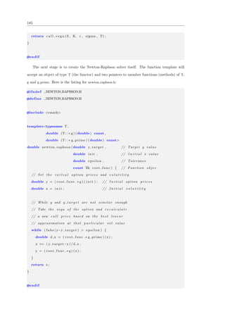
14.2.2 Implementing a Linear Congruential Generator
With the mathematical algorithm described, it is straightforward to create the header file listing
(lin con gen.h) for the Linear Congruential Generator. The LCG simply inherits from the RNG
abstract base class, adds a private member variable called max multiplier (used for pre-computing
a specific ratio required in the uniform draw implementation) and implements the two pure virtual
methods that were part of the RNG abstract base class:
#ifndef LINEAR CONGRUENTIAL GENERATOR H
#define LINEAR CONGRUENTIAL GENERATOR H
#include ”random . h”
class LinearCongruentialGenerator : public RandomNumberGenerator {
private :
double max multiplier ;
public :
LinearCongruentialGenerator (unsigned long num draws ,
unsigned long i n i t s e e d = 1) ;
virtual ˜ LinearCongruentialGenerator () {};
virtual unsigned long get random integer () ;
virtual void get uniform draws ( std : : vector<double> draws ) ;
};
#endif
The source file (lin con gen.cpp) contains the implementation of the linear congruential gen-
erator algorithm. We make heavy use of Numerical Recipes in C[20], the famed numerical
algorithms cookbook. The book itself is freely available online. I would strongly suggest reading
the chapter on random number generator (Chapter 7) as it describes many of the pitfalls with
using a basic linear congruential generator, which I do not have time to elucidate on in this
chapter. Here is the listing in full:
#ifndef LINEAR CONGRUENTIAL GENERATOR CPP
#define LINEAR CONGRUENTIAL GENERATOR CPP
#include ” l i n c o n g e n . h”](https://image.slidesharecdn.com/266803730-cpp-quant-finance-ebook-20131003-180810164750/85/C-For-Quantitative-Finance-195-320.jpg)

![196
}
// Create a vector of uniform draws between (0 ,1)
void LinearCongruentialGenerator : : get uniform draws ( std : : vector<double>&
draws ) {
for ( unsigned long i =0; i<num draws ; i++) {
draws [ i ] = get random integer () ∗ max multiplier ;
}
}
#endif
Firstly, we set all of the necessary constants (see [20] for the explanation of the chosen values).
Note that if we created another LCG we could inherit from the RNG base class and use different
constants:
// Define the constants for the Park & Miller algorithm
const unsigned long a = 16807; // 7ˆ5
const unsigned long m = 2147483647; // 2ˆ32 − 1
// Schrage ’ s algorithm constants
const unsigned long q = 127773;
const unsigned long r = 2836;
Secondly we implement the constructor for the LCG. If the seed is set to zero by the client,
we set it to unity, as the LCG algorithm does not work with a seed of zero. The max mutliplier is
a pre-computed scaling factor necessary for converting a random unsigned long into a uniform
value on on the open interval (0, 1) ⊂ R:
// Parameter constructor
LinearCongruentialGenerator : : LinearCongruentialGenerator (
unsigned long num draws ,
unsigned long i n i t s e e d
) : RandomNumberGenerator ( num draws , i n i t s e e d ) {
i f ( i n i t s e e d == 0) {
i n i t s e e d = 1;](https://image.slidesharecdn.com/266803730-cpp-quant-finance-ebook-20131003-180810164750/85/C-For-Quantitative-Finance-197-320.jpg)
![197
cur seed = 1;
}
max multiplier = 1.0 / ( 1. 0 + (m−1)) ;
}
We now concretely implement the two pure virtual functions of the RNG base class, namely
get random integer and get uniform draws. get random integer applies the LCG modulus algorithm
and modifies the current seed (as described in the algorithm above):
// Obtains a random unsigned long i n t e g e r
unsigned long LinearCongruentialGenerator : : get random integer () {
unsigned long k = 0;
k = cur seed / q ;
cur seed = a ∗ ( cur seed − k ∗ q) − r ∗ k ;
i f ( cur seed < 0) {
cur seed += m;
}
return cur seed ;
}
get uniform draws takes in a vector of the correct length (num draws) and loops over it con-
verting random integers generated by the LCG into uniform random variables on the interval
(0, 1):
// Create a vector of uniform draws between (0 ,1)
void LinearCongruentialGenerator : : get uniform draws ( std : : vector<double>&
draws ) {
for ( unsigned long i =0; i<num draws ; i++) {
draws [ i ] = get random integer () ∗ max multiplier ;
}
}
The concludes the implementation of the linear congruential generator. The final component
is to tie it all together with a main.cpp program.](https://image.slidesharecdn.com/266803730-cpp-quant-finance-ebook-20131003-180810164750/85/C-For-Quantitative-Finance-198-320.jpg)
![198
14.2.3 Implementation of the Main Program
Because we have already carried out most of the hard work in random.h, lin con gen.h, lin con gen
.cpp, the main implementation (main.cpp) is straightforward:
#include <iostream>
#include ” l i n c o n g e n . h”
int main ( int argc , char ∗∗ argv ) {
// Set the i n i t i a l seed and the dimensionality of the RNG
unsigned long i n i t s e e d = 1;
unsigned long num draws = 20;
std : : vector<double> random draws ( num draws , 0 .0 ) ;
// Create the LCG o b j e c t and create the random uniform draws
// on the open i n t e r v a l (0 ,1)
LinearCongruentialGenerator lcg ( num draws , i n i t s e e d ) ;
lcg . get uniform draws ( random draws ) ;
// Output the random draws to the console / stdout
for ( unsigned long i =0; i<num draws ; i++) {
std : : cout << random draws [ i ] << std : : endl ;
}
return 0;
}
Firstly, we set up the initial seed and the dimensionality of the random number genera-
tor. Then we pre-initialise the vector, which will ultimately contain the uniform draws. Then
we instantiate the linear congruential generator and pass the random draws vector into the
get uniform draws method. Finally we output the uniform variables. The output of the code
is as follows:
7.82637 e−06
0.131538
0.755605
0.45865
0.532767
0.218959](https://image.slidesharecdn.com/266803730-cpp-quant-finance-ebook-20131003-180810164750/85/C-For-Quantitative-Finance-199-320.jpg)


![202
tion is given by:
φ(x) =
1
√
2π
e− 1
2 x2
The cumulative density function is given by:
Φ(x) =
1
√
2π
x
−∞
e− t2
2 dt
The inverse cumulative density function of the standard normal distribution (also known as
the probit function) is somewhat more involved. No analytical formula exists for this particular
function and so it must be approximated by numerical methods. We will utilise the Beasley-
Springer-Moro algorithm, found in Korn[15].
Given that we are dealing with the standard normal distribution, the mean is simply µ = 0,
variance σ2
= 1 and standard deviation, σ = 1. The implementation for the header file (which
is a continuation of statistics .h above) is as follows:
class StandardNormalDistribution : public S t a t i s t i c a l D i s t r i b u t i o n {
public :
StandardNormalDistribution () ;
virtual ˜ StandardNormalDistribution () ;
// D i s t r i b u t i o n functions
virtual double pdf ( const double& x) const ;
virtual double cdf ( const double& x) const ;
// Inverse cumulative d i s t r i b u t i o n function ( aka the p r o b i t function )
virtual double i nv c d f ( const double& quantile ) const ;
// Descriptive s t a t s
virtual double mean () const ; // equal to 0
virtual double var () const ; // equal to 1
virtual double stdev () const ; // equal to 1
// Obtain a sequence of random draws from the standard normal
d i s t r i b u t i o n](https://image.slidesharecdn.com/266803730-cpp-quant-finance-ebook-20131003-180810164750/85/C-For-Quantitative-Finance-203-320.jpg)

![204
// Inverse cumulative d i s t r i b u t i o n function ( aka the p r o b i t function )
double StandardNormalDistribution : : i n v c df ( const double& quantile ) const {
// This i s the Beasley−Springer−Moro algorithm which can
// be found in Glasserman [ 2 0 0 4 ] . We won ’ t go into the
// d e t a i l s here , so have a look at the reference for more info
static double a [ 4 ] = { 2.50662823884 ,
−18.61500062529 ,
41.39119773534 ,
−25.44106049637};
static double b [ 4 ] = { −8.47351093090 ,
23.08336743743 ,
−21.06224101826 ,
3.13082909833};
static double c [ 9 ] = {0.3374754822726147 ,
0.9761690190917186 ,
0.1607979714918209 ,
0.0276438810333863 ,
0.0038405729373609 ,
0.0003951896511919 ,
0.0000321767881768 ,
0.0000002888167364 ,
0.0000003960315187};
i f ( quantile >= 0.5 && quantile <= 0.92) {
double num = 0 . 0 ;
double denom = 1 . 0 ;
for ( int i =0; i <4; i++) {
num += a [ i ] ∗ pow (( quantile − 0 .5 ) , 2∗ i + 1) ;
denom += b [ i ] ∗ pow (( quantile − 0 .5 ) , 2∗ i ) ;
}
return num/denom ;
} else i f ( quantile > 0.92 && quantile < 1) {](https://image.slidesharecdn.com/266803730-cpp-quant-finance-ebook-20131003-180810164750/85/C-For-Quantitative-Finance-205-320.jpg)
![205
double num = 0 . 0 ;
for ( int i =0; i <9; i++) {
num += c [ i ] ∗ pow (( log(−log (1− quantile ) ) ) , i ) ;
}
return num;
} else {
return −1.0∗ i nv c df (1− quantile ) ;
}
}
// Expectation /mean
double StandardNormalDistribution : : mean () const { return 0 . 0 ; }
// Variance
double StandardNormalDistribution : : var () const { return 1 . 0 ; }
// Standard Deviation
double StandardNormalDistribution : : stdev () const { return 1 . 0 ; }
// Obtain a sequence of random draws from t h i s d i s t r i b u t i o n
void StandardNormalDistribution : : random draws (
const std : : vector<double>& uniform draws ,
std : : vector<double>& dist draws
) {
// The simplest method to c a l c u l a t e t h i s i s with the Box−Muller method ,
// which has been used procedurally in many other chapters
// Check that the uniform draws and dist draws are the same s i z e and
// have an even number of elements ( necessary for B−M)
i f ( uniform draws . s i z e () != dist draws . s i z e () ) {
std : : cout << ”Draw vectors are of unequal s i z e . ” << std : : endl ;
return ;
}
// Check that uniform draws have an even number of elements ( necessary](https://image.slidesharecdn.com/266803730-cpp-quant-finance-ebook-20131003-180810164750/85/C-For-Quantitative-Finance-206-320.jpg)
![206
for B−M)
i f ( uniform draws . s i z e () % 2 != 0) {
std : : cout << ”Uniform draw vector s i z e not an even number . ” << std : :
endl ;
return ;
}
// Slow , but easy to implement
for ( int i =0; i<uniform draws . s i z e () / 2; i++) {
dist draws [2∗ i ] = sqrt ( −2.0∗ log ( uniform draws [2∗ i ] ) ) ∗
sin (2∗M PI∗ uniform draws [2∗ i +1]) ;
dist draws [2∗ i +1] = sqrt ( −2.0∗ log ( uniform draws [2∗ i ] ) ) ∗
cos (2∗M PI∗ uniform draws [2∗ i +1]) ;
}
return ;
}
#endif
I’ll discuss briefly some of the implementations here. The cumulative distribution function
(cdf) is referenced from Joshi[12]. It is an approximation, rather than closed-form solution. The
inverse CDF (inv cdf) makes use of the Beasley-Springer-Moro algorithm, which was implemented
via the algorithm given in Korn[15]. A similar method can be found in Joshi[11]. Once again
the algorithm is an approximation to the real function, rather than a closed form solution. The
final method is random draws. In this instance we are using the Box-Muller algorithm. However,
we could instead utilise the more efficient Ziggurat algorithm, although we won’t do so here.
14.3.3 The Main Listing
We will now utilise the new statistical distribution classes with a simple random number generator
in order to output statistical values:
#include ” s t a t i s t i c s . h”
#include <iostream>
#include <vector>
int main ( int argc , char ∗∗ argv ) {](https://image.slidesharecdn.com/266803730-cpp-quant-finance-ebook-20131003-180810164750/85/C-For-Quantitative-Finance-207-320.jpg)
![207
// Create the Standard Normal D i s t r i b u t i o n and random draw vectors
StandardNormalDistribution snd ;
std : : vector<double> uniform draws (20 , 0 . 0) ;
std : : vector<double> normal draws (20 , 0 .0 ) ;
// Simple random number generation method based on RAND
for ( int i =0; i<uniform draws . s i z e () ; i++) {
uniform draws [ i ] = rand () / static cast<double>(RANDMAX) ;
}
// Create standard normal random draws
// Notice that the uniform draws are unaffected . We have separated
// out the uniform creation from the normal draw creation , which
// w i l l allow us to create s o p h i s t i c a t e d random number generators
// without i n t e r f e r i n g with the s t a t i s t i c a l c l a s s e s
snd . random draws ( uniform draws , normal draws ) ;
// Output the values of the standard normal random draws
for ( int i =0; i<normal draws . s i z e () ; i++) {
std : : cout << normal draws [ i ] << std : : endl ;
}
return 0;
}
The output from the program is as follows (a sequence of normally distributed random vari-
ables):
3.56692
3.28529
0.192324
−0.723522
1.10093
0.217484
−2.22963
−1.06868
−0.35082
0.806425](https://image.slidesharecdn.com/266803730-cpp-quant-finance-ebook-20131003-180810164750/85/C-For-Quantitative-Finance-208-320.jpg)

![Chapter 15
Jump-Diffusion Models
This chapter will deal with a particular assumption of the Black-Scholes model and how to refine
it to produce more accurate pricing models. In the Black-Scholes model the stock price evolves
as a geometric Brownian motion. Crucially, this allows continuous Delta hedging and thus a
fixed no-arbitrage price for any option on the stock.
If we relax the assumption of GBM and introduce the concept of discontinuous jumps in the
stock price then it becomes impossible to perfectly hedge and leads to market incompleteness.
This means that options prices are only bounded rather than fixed. In this article we will consider
the effect on options prices when such jumps occur and implement a semi-closed form pricer in
C++ based on the analytical formula derived by Merton[16].
15.1 Modelling Jump-Diffusion Processes
This section closely follows the chapter on Jump Diffusions in Joshi[12], where more theoretical
details are provided.
In order to model such stock ”jumps” we require certain properties. Firstly, the jumps
should occur in an instantaneous fashion, neglecting the possibility of a Delta hedge. Secondly,
we require that the probability of any jump occuring in a particular interval of time should
be approximately proportional to the length of that time interval. The statistical method that
models such a situation is given by the Poisson process[12].
A Poisson process states the probability of an event occuring in a given time interval ∆t is
given by λ∆t+ , where λ is the intensity of the process and is an error term. The integer-valued
number of events that have occured at time t is given by N(t). A necessary property is that the
probability of a jump occuring is independent of the number of jumps already occured, i.e. all
209](https://image.slidesharecdn.com/266803730-cpp-quant-finance-ebook-20131003-180810164750/85/C-For-Quantitative-Finance-210-320.jpg)
![210
future jumps should have no ”memory” of past jumps. The probability of j jumps occuring by
time t is given by:
P(N(t) = j) =
(λt)j
j!
e−λt
(15.1)
Thus, we simply need to modify our underlying GBM model for the stock via the addition of
jumps. This is achieved by allowing the stock price to be multiplied by a random factor J:
dSt = µStdt + σStdWt + (J − 1)StdN(t) (15.2)
Where dN(t) is Poisson distributed with factor λdt.
15.2 Prices of European Options under Jump-Diffusions
After an appropriate application of risk neutrality[12] we have that log ST , the log of the final
price of the stock at option expiry, is given by:
log(ST ) = log(S0) + µ +
1
2
σ2
T + σ
√
TN(0, 1) +
N(T )
j=1
logJj (15.3)
This is all we need to price European options under a Monte Carlo framework. To carry
this out we simply generate multiple final spot prices by drawing from a normal distribution
and a Poisson distribution, and then selecting the Jj values to form the jumps. However, this is
somewhat unsatisfactory as we are specifically choosing the Jj values for the jumps. Shouldn’t
they themselves also be random variables distributed in some manner?
In 1976, Robert Merton[16] was able to derive a semi-closed form solution for the price of
European options where the jump values are themselves normally distributed. If the price of an
option priced under Black-Scholes is given by BS(S0, σ, r, T, K) with S0 initial spot, σ constant
volatility, r constant risk-free rate, T time to maturity and K strike price, then in the jump-
diffusion framework the price is given by[12]:
∞
n=0
e−λ T
(λ T)n
n!
BS(S0, σn, rn, T, K) (15.4)](https://image.slidesharecdn.com/266803730-cpp-quant-finance-ebook-20131003-180810164750/85/C-For-Quantitative-Finance-211-320.jpg)


![219
// This c a r r i e s out the actual c o r r e l a t i o n modification . I t i s easy to see
that i f
// rho = 0.0 , then dist draws i s unmodified , whereas i f rho = 1.0 , then
dist draws
// i s simply s e t equal to uncorr draws . Thus with 0 < rho < 1 we have a
// weighted average of each s e t .
void CorrelatedSND : : c o r r e l a t i o n c a l c ( std : : vector<double>& dist draws ) {
for ( int i =0; i<dist draws . s i z e () ; i++) {
dist draws [ i ] = rho ∗ (∗ uncorr draws ) [ i ] + dist draws [ i ] ∗ sqrt (1−rho
∗rho ) ;
}
}
void CorrelatedSND : : random draws ( const std : : vector<double>& uniform draws ,
std : : vector<double>>& dist draws ) {
// The f o l l o w i n g f u n c t i o n a l i t y i s l i f t e d d i r e c t l y from
// s t a t i s t i c s . h , which i s f u l l y commented !
i f ( uniform draws . s i z e () != dist draws . s i z e () ) {
std : : cout << ”Draws vectors are of unequal s i z e in standard normal d i s t
. ”
<< std : : endl ;
return ;
}
i f ( uniform draws . s i z e () % 2 != 0) {
std : : cout << ”Uniform draw vector s i z e not an even number . ” << std : :
endl ;
return ;
}
for ( int i =0; i<uniform draws . s i z e () / 2; i++) {
dist draws [2∗ i ] = sqrt ( −2.0∗ log ( uniform draws [2∗ i ] ) ) ∗
sin (2∗M PI∗ uniform draws [2∗ i +1]) ;
dist draws [2∗ i +1] = sqrt ( −2.0∗ log ( uniform draws [2∗ i ] ) ) ∗
cos (2∗M PI∗ uniform draws [2∗ i +1]) ;
}](https://image.slidesharecdn.com/266803730-cpp-quant-finance-ebook-20131003-180810164750/85/C-For-Quantitative-Finance-220-320.jpg)

![221
// random number generation !
for ( int i =0; i<snd uniform draws . s i z e () ; i++) {
snd uniform draws [ i ] = rand () / static cast<double>(RANDMAX) ;
}
// Create standard normal random draws
snd . random draws ( snd uniform draws , snd normal draws ) ;
/∗ CORRELATION SND ∗/
/∗ =============== ∗/
// Correlation c o e f f i c i e n t
double rho = 0 . 5 ;
// Create the c o r r e l a t e d standard normal d i s t r i b u t i o n
CorrelatedSND csnd ( rho , &snd normal draws ) ;
std : : vector<double> csnd uniform draws ( vals , 0 .0 ) ;
std : : vector<double> csnd normal draws ( vals , 0 .0 ) ;
// Uniform generation for the c o r r e l a t e d SND
for ( int i =0; i<csnd uniform draws . s i z e () ; i++) {
csnd uniform draws [ i ] = rand () / static cast<double>(RANDMAX) ;
}
// Now create the −correlated − standard normal draw s e r i e s
csnd . random draws ( csnd uniform draws , csnd normal draws ) ;
// Output the values of the standard normal random draws
for ( int i =0; i<snd normal draws . s i z e () ; i++) {
std : : cout << snd normal draws [ i ] << ” , ” << csnd normal draws [ i ] << std
: : endl ;
}
return 0;
}
The above code is somewhat verbose, but that is simply a consequence of not encapsulating](https://image.slidesharecdn.com/266803730-cpp-quant-finance-ebook-20131003-180810164750/85/C-For-Quantitative-Finance-222-320.jpg)


![230
// Calculate the v o l a t i l i t y path
void c a l c v o l p a t h ( const std : : vector<double>& vol draws ,
std : : vector<double>& vol path ) ;
// Calculate the a s se t price path
void calc spot path ( const std : : vector<double>& spot draws ,
const std : : vector<double>& vol path ,
std : : vector<double>& spot path ) ;
};
#endif
The listing for heston mc.cpp follows:
#ifndef HESTON MC CPP
#define HESTON MC CPP
#include ”heston mc . h”
// HestonEuler
// ===========
HestonEuler : : HestonEuler ( Option∗ pOption ,
double kappa , double theta ,
double xi , double rho ) :
pOption ( pOption ) , kappa ( kappa ) , theta ( theta ) , xi ( x i ) , rho ( rho ) {}
HestonEuler : : ˜ HestonEuler () {}
void HestonEuler : : c a l c v o l p a t h ( const std : : vector<double>& vol draws ,
std : : vector<double>& vol path ) {
s i z e t v e c s i z e = vol draws . s i z e () ;
double dt = pOption−>T/ static cast<double>( v e c s i z e ) ;
// I t e r a t e through the c o r r e l a t e d random draws vector and
// use the ’ Full Truncation ’ scheme to create the v o l a t i l i t y path
for ( int i =1; i<v e c s i z e ; i++) {
double v max = std : : max( vol path [ i −1] , 0. 0 ) ;](https://image.slidesharecdn.com/266803730-cpp-quant-finance-ebook-20131003-180810164750/85/C-For-Quantitative-Finance-231-320.jpg)
![231
vol path [ i ] = vol path [ i −1] + kappa ∗ dt ∗ ( theta − v max ) +
xi ∗ sqrt ( v max ∗ dt ) ∗ vol draws [ i −1];
}
}
void HestonEuler : : calc spot path ( const std : : vector<double>& spot draws ,
const std : : vector<double>& vol path ,
std : : vector<double>& spot path ) {
s i z e t v e c s i z e = spot draws . s i z e () ;
double dt = pOption−>T/ static cast<double>( v e c s i z e ) ;
// Create the spot price path making use of the v o l a t i l i t y
// path . Uses a s i m i l a r Euler Truncation method to the vol path .
for ( int i =1; i<v e c s i z e ; i++) {
double v max = std : : max( vol path [ i −1] , 0. 0 ) ;
spot path [ i ] = spot path [ i −1] ∗ exp ( ( pOption−>r − 0.5∗ v max ) ∗dt +
sqrt ( v max∗dt ) ∗ spot draws [ i −1]) ;
}
}
#endif
The calc vol path method takes references to a const vector of normal draws and a vector
to store the volatility path. It calculates the ∆t value (as dt), based on the option maturity
time. Then, the stochastic simulation of the volatility path is carried out by means of the Full
Truncation Euler Discretisation, outlined in the mathematical treatment above. Notice that ν+
i
is precalculated, for efficiency reasons.
The calc spot path method is similar to the calc vol path method, with the exception that it
accepts another vector, vol path that contains the volatility path values at each time increment.
The risk-free rate r is obtained from the option pointer and, once again, ν+
i is precalculated.
Note that all vectors are passed by reference in order to reduce unnecessary copying.
16.7.5 Main Program
This is where it all comes together. There are two components to this listing: The generate normal correlation paths
function and the main function. The former is designed to handle the ”boilerplate” code of gen-
erating the necessary uniform random draw vectors and then utilising the CorrelatedSND object](https://image.slidesharecdn.com/266803730-cpp-quant-finance-ebook-20131003-180810164750/85/C-For-Quantitative-Finance-232-320.jpg)
![232
to produce correlated standard normal distribution random draw vectors.
I wanted to keep this entire example of the Heston model tractable, so I have simply used
the C++ built-in rand function to produce the uniform standard draws. However, in a pro-
duction environment a Mersenne Twister uniform number generator (or something even more
sophisticated) would be used to produce high-quality pseudo-random numbers. The output of
the function is to calculate the values for the spot normals and cor normals vectors, which are
used by the asset spot path and the volatility path respectively.
The main function begins by defining the parameters of the simulation, including the Monte
Carlo values and those necessary for the option and Heston model. The actual parameter values
are those give in the paper by Broadie and Kaya[3]. The next task is to create the pointers to
the PayOff and Option classes, as well as the HestonEuler instance itself.
After declaration of the various vectors used to hold the path values, a basic Monte Carlo
loop is created. For each asset simulation, the new correlated values are generated, leading to
the calculation of the vol path and the asset spot path. The option pay-off is calculated for
each path and added to the total, which is then subsequently averaged and discounted via the
risk-free rate. The option price is output to the terminal and finally the pointers are deleted.
Here is the listing for main.cpp:
#include <iostream>
#include ” payoff . h”
#include ” option . h”
#include ” co rr el ate d sn d . h”
#include ”heston mc . h”
void generate normal correlation paths (double rho ,
std : : vector<double>& spot normals , std : : vector<double>& cor normals ) {
unsigned vals = spot normals . s i z e () ;
// Create the Standard Normal D i s t r i b u t i o n and random draw vectors
StandardNormalDistribution snd ;
std : : vector<double> snd uniform draws ( vals , 0. 0 ) ;
// Simple random number generation method based on RAND
for ( int i =0; i<snd uniform draws . s i z e () ; i++) {
snd uniform draws [ i ] = rand () / static cast<double>(RANDMAX) ;](https://image.slidesharecdn.com/266803730-cpp-quant-finance-ebook-20131003-180810164750/85/C-For-Quantitative-Finance-233-320.jpg)
![233
}
// Create standard normal random draws
snd . random draws ( snd uniform draws , spot normals ) ;
// Create the c o r r e l a t e d standard normal d i s t r i b u t i o n
CorrelatedSND csnd ( rho , &spot normals ) ;
std : : vector<double> csnd uniform draws ( vals , 0 .0 ) ;
// Uniform generation for the c o r r e l a t e d SND
for ( int i =0; i<csnd uniform draws . s i z e () ; i++) {
csnd uniform draws [ i ] = rand () / static cast<double>(RANDMAX) ;
}
// Now create the −correlated − standard normal draw s e r i e s
csnd . random draws ( csnd uniform draws , cor normals ) ;
}
int main ( int argc , char ∗∗ argv ) {
// F i rs t we create the parameter l i s t
// Note that you could e a s i l y modify t h i s code to input the parameters
// e i t h e r from the command l i n e or via a f i l e
unsigned num sims = 100000; // Number of simulated a s s e t paths
unsigned num intervals = 1000; // Number of i n t e r v a l s for the a s s e t path
to be sampled
double S 0 = 1 0 0 . 0 ; // I n i t i a l spot price
double K = 1 0 0 . 0 ; // S t r i k e price
double r = 0.0319; // Risk−f r e e rate
double v 0 = 0.010201; // I n i t i a l v o l a t i l i t y
double T = 1 . 0 0 ; // One year u n t i l expiry
double rho = −0.7; // Correlation of a s se t and v o l a t i l i t y
double kappa = 6 . 2 1 ; // Mean−reversion rate
double theta = 0 . 0 1 9 ; // Long run average v o l a t i l i t y
double xi = 0 . 6 1 ; // ”Vol of vol ”](https://image.slidesharecdn.com/266803730-cpp-quant-finance-ebook-20131003-180810164750/85/C-For-Quantitative-Finance-234-320.jpg)
![234
// Create the PayOff , Option and Heston o b j e c t s
PayOff∗ pPayOffCall = new PayOffCall (K) ;
Option∗ pOption = new Option (K, r , T, pPayOffCall ) ;
HestonEuler h e s t e u l e r ( pOption , kappa , theta , xi , rho ) ;
// Create the spot and vol i n i t i a l normal and price paths
std : : vector<double> spot draws ( num intervals , 0 .0 ) ; // Vector of i n i t i a l
spot normal draws
std : : vector<double> vol draws ( num intervals , 0 .0 ) ; // Vector of i n i t i a l
c o r r e l a t e d vol normal draws
std : : vector<double> s p o t p r i c e s ( num intervals , S 0 ) ; // Vector of
i n i t i a l spot p r i c e s
std : : vector<double> v o l p r i c e s ( num intervals , v 0 ) ; // Vector of
i n i t i a l vol p r i c e s
// Monte Carlo options p r i c i n g
double payoff sum = 0 . 0 ;
for ( unsigned i =0; i<num sims ; i++) {
std : : cout << ” Calculating path ” << i+1 << ” of ” << num sims << std : :
endl ;
generate normal correlation paths ( rho , spot draws , vol draws ) ;
h e s t e u l e r . c a l c v o l p a t h ( vol draws , v o l p r i c e s ) ;
h e s t e u l e r . calc spot path ( spot draws , v o l p r i c e s , s p o t p r i c e s ) ;
payoff sum += pOption−>pay off −>operator () ( s p o t p r i c e s [ num intervals
−1]) ;
}
double o p t i o n p r i c e = ( payoff sum / static cast<double>(num sims ) ) ∗ exp
(−r ∗T) ;
std : : cout << ”Option Price : ” << o p t i o n p r i c e << std : : endl ;
// Free memory
delete pOption ;
delete pPayOffCall ;
return 0;
}](https://image.slidesharecdn.com/266803730-cpp-quant-finance-ebook-20131003-180810164750/85/C-For-Quantitative-Finance-235-320.jpg)
![235
For completeness, I have included the makefile utilised on my MacBook Air, running Mac
OSX 10.7.4:
heston : main . cpp heston mc . o co rr ela te d s nd . o s t a t i s t i c s . o option . o payoff .
o
clang++ −o heston main . cpp heston mc . o co rr ela te d s nd . o s t a t i s t i c s . o
option . o payoff . o −arch x86 64
heston mc . o : heston mc . cpp option . o
clang++ −c heston mc . cpp option . o −arch x86 64
co rr el at ed sn d . o : cor re la te d sn d . cpp s t a t i s t i c s . o
clang++ −c c orr el at ed s nd . cpp s t a t i s t i c s . o −arch x86 64
s t a t i s t i c s . o : s t a t i s t i c s . cpp
clang++ −c s t a t i s t i c s . cpp −arch x86 64
option . o : option . cpp payoff . o
clang++ −c option . cpp payoff . o −arch x86 64
payoff . o : payoff . cpp
clang++ −c payoff . cpp −arch x86 64
Here is the output of the program:
. .
. .
Calculating path 99997 of 100000
Calculating path 99998 of 100000
Calculating path 99999 of 100000
Calculating path 100000 of 100000
Option Price : 6.81982
The exact option price is 6.8061, as reported by Broadie and Kaya[3]. It can be made
somewhat more accurate by increasing the number of asset paths and discretisation intervals.
There are a few extensions that could be made at this stage. One is to allow the various
”schemes” to be implemented, rather than hard-coded as above. Another is to introduce time-
dependence into the parameters. The next step after creating a model of this type is to actually
calibrate to a set of market data such that the parameters may be determined.](https://image.slidesharecdn.com/266803730-cpp-quant-finance-ebook-20131003-180810164750/85/C-For-Quantitative-Finance-236-320.jpg)


![249
protected :
ConvectionDiffusionPDE ∗ pde ;
// Space d i s c r e t i s a t i o n
double x dom ; // S p a t i a l extent [ 0 . 0 , x dom ]
unsigned long J ; // Number of s p a t i a l d i f f e r e n c i n g points
double dx ; // S p a t i a l step s i z e ( c a l c u l a t e d from above )
std : : vector<double> x values ; // Stores the coordinates of the x
dimension
// Time d i s c r e t i s a t i o n
double t dom ; // Temporal extent [ 0 . 0 , t dom ]
unsigned long N; // Number of temporal d i f f e r e n c i n g points
double dt ; // Temporal step s i z e ( c a l c u l a t e d from above )
// Time−marching
double prev t , cur t ; // Current and previous times
// Differencing c o e f f i c i e n t s
double alpha , beta , gamma;
// Storage
std : : vector<double> new result ; // New s o l u t i o n ( becomes N+1)
std : : vector<double> o l d r e s u l t ; // Old s o l u t i o n ( becomes N)
// Constructor
FDMBase(double x dom , unsigned long J ,
double t dom , unsigned long N ,
ConvectionDiffusionPDE ∗ pde ) ;
// Override these v i r t u a l methods in derived c l a s s e s for
// s p e c i f i c FDM techniques , such as e x p l i c i t Euler , Crank−Nicolson , etc .
virtual void c a l c u l a t e s t e p s i z e s () = 0;
virtual void s e t i n i t i a l c o n d i t i o n s () = 0;
virtual void calculate boundary conditions () = 0;
virtual void calculate inner domain () = 0;](https://image.slidesharecdn.com/266803730-cpp-quant-finance-ebook-20131003-180810164750/85/C-For-Quantitative-Finance-250-320.jpg)

![251
ConvectionDiffusionPDE ∗ pde )
: FDMBase( x dom , J , t dom , N , pde ) {
c a l c u l a t e s t e p s i z e s () ;
s e t i n i t i a l c o n d i t i o n s () ;
}
void FDMEulerExplicit : : c a l c u l a t e s t e p s i z e s () {
dx = x dom/ static cast<double>(J−1) ;
dt = t dom/ static cast<double>(N−1) ;
}
void FDMEulerExplicit : : s e t i n i t i a l c o n d i t i o n s () {
// S p a t i a l s e t t i n g s
double cur spot = 0 . 0 ;
o l d r e s u l t . r e s i z e (J , 0 . 0 ) ;
new result . r e s i z e (J , 0 . 0 ) ;
x values . r e s i z e (J , 0. 0 ) ;
for ( unsigned long j =0; j<J ; j++) {
cur spot = static cast<double>( j ) ∗dx ;
o l d r e s u l t [ j ] = pde−>i n i t c o n d ( cur spot ) ;
x values [ j ] = cur spot ;
}
// Temporal s e t t i n g s
prev t = 0 . 0 ;
cur t = 0 . 0 ;
}
void FDMEulerExplicit : : calculate boundary conditions () {
new result [ 0 ] = pde−>boundary left ( prev t , x values [ 0 ] ) ;
new result [ J−1] = pde−>boundary right ( prev t , x values [ J −1]) ;
}
void FDMEulerExplicit : : calculate inner domain () {
// Only use inner r e s u l t i n d i c e s (1 to J−2)](https://image.slidesharecdn.com/266803730-cpp-quant-finance-ebook-20131003-180810164750/85/C-For-Quantitative-Finance-252-320.jpg)
![252
for ( unsigned long j =1; j<J−1; j++) {
// Temporary v a r i a b l e s used throughout
double d t s i g = dt ∗ ( pde−>d i f f c o e f f ( prev t , x values [ j ] ) ) ;
double d t s i g 2 = dt ∗ dx ∗ 0.5 ∗ ( pde−>c on v c oe ff ( prev t , x values [ j ] )
) ;
// Differencing c o e f f i c i e n t s ( see alpha , beta and gamma in t e x t )
alpha = d t s i g − d t s i g 2 ;
beta = dx ∗ dx − ( 2. 0 ∗ d t s i g ) + ( dt ∗ dx ∗ dx ∗
( pde−>z e r o c o e f f ( prev t , x values [ j ] ) ) ) ;
gamma = d t s i g + d t s i g 2 ;
// Update inner values of s p a t i a l d i s c r e t i s a t i o n grid ( E x p l i c i t Euler )
new result [ j ] = ( ( alpha ∗ o l d r e s u l t [ j −1]) +
( beta ∗ o l d r e s u l t [ j ] ) +
(gamma ∗ o l d r e s u l t [ j +1]) ) /(dx∗dx) −
( dt ∗( pde−>s o u r c e c o e f f ( prev t , x values [ j ] ) ) ) ;
}
}
void FDMEulerExplicit : : step march () {
std : : ofstream fdm out ( ”fdm . csv ” ) ;
while ( cur t < t dom ) {
cur t = prev t + dt ;
calculate boundary conditions () ;
calculate inner domain () ;
for ( int j =0; j<J ; j++) {
fdm out << x values [ j ] << ” ” << prev t << ” ”
<< new result [ j ] << std : : endl ;
}
o l d r e s u l t = new result ;
prev t = cur t ;
}
fdm out . c l o s e () ;](https://image.slidesharecdn.com/266803730-cpp-quant-finance-ebook-20131003-180810164750/85/C-For-Quantitative-Finance-253-320.jpg)

![254
the pointer to the PDE to obtain the initial condition as a function of spot. We also have a
useful ”helper” array, x values which stores the spot value at each discretisation point to save us
calculating it every time step. Finally, we set the current and previous times to zero:
void FDMEulerExplicit : : s e t i n i t i a l c o n d i t i o n s () {
// S p a t i a l s e t t i n g s
double cur spot = 0 . 0 ;
o l d r e s u l t . r e s i z e (J , 0. 0 ) ;
new result . r e s i z e (J , 0 . 0 ) ;
x values . r e s i z e (J , 0. 0 ) ;
for ( unsigned long j =0; j<J ; j++) {
cur spot = static cast<double>( j ) ∗dx ;
o l d r e s u l t [ j ] = pde−>i n i t c o n d ( cur spot ) ;
x values [ j ] = cur spot ;
}
// Temporal s e t t i n g s
prev t = 0 . 0 ;
cur t = 0 . 0 ;
}
Now that the initial conditions are set we can begin the time-marching. However, in each
time step we must first set the boundary conditions. In this instance the edge points (at index
0 and index J − 1) are set using the PDE boundary left and boundary right method. This is
an example of a Dirichlet condition. More sophisticated boundary conditions approximate the
derivative at these points (Neumann conditions), although we won’t be utilising these conditions
here:
void FDMEulerExplicit : : calculate boundary conditions () {
new result [ 0 ] = pde−>boundary left ( prev t , x values [ 0 ] ) ;
new result [ J−1] = pde−>boundary right ( prev t , x values [ J −1]) ;
}
The ”meat” of the FDM solver occurs in the calculate inner domain method. Let’s run through
how it works. A loop is carried out over the spatial cells - but only those away from the boundary,
hence the index 1 to J − 2. In order to save excessive repetitive calculation (and enhance
readability), we create two helper variables called dt sig and dt sig 2. If you refer back to the](https://image.slidesharecdn.com/266803730-cpp-quant-finance-ebook-20131003-180810164750/85/C-For-Quantitative-Finance-255-320.jpg)
![255
mathematical formalism at the start of the chapter, it will be apparent where these variables
arise from.
The next step is to calculate the α, β and γ coefficients which represent the algebraic re-
arrangement of the derivative discretisation. Again, these terms will be clear from the above
mathematical formalism. In fact, I’ve tried to make the C++ implementation as close as possi-
ble to the mathematical algorithm in order to make it easier to follow! Notice that we need to
obtain certain coefficients via pointer dereferencing of the underlying PDE.
Once α, β and γ are defined we can use the finite differencing to update the solution into the
new result vector. This formula will also be clear from the mathematical algorithm above:
void FDMEulerExplicit : : calculate inner domain () {
// Only use inner r e s u l t i n d i c e s (1 to J−2)
for ( unsigned long j =1; j<J−1; j++) {
// Temporary v a r i a b l e s used throughout
double d t s i g = dt ∗ ( pde−>d i f f c o e f f ( prev t , x values [ j ] ) ) ;
double d t s i g 2 = dt ∗ dx ∗ 0.5 ∗ ( pde−>c on v c oe ff ( prev t , x values [ j ] )
) ;
// Differencing c o e f f i c i e n t s ( see alpha , beta and gamma in t e x t )
alpha = d t s i g − d t s i g 2 ;
beta = dx ∗ dx − ( 2 .0 ∗ d t s i g ) + ( dt ∗ dx ∗ dx ∗
( pde−>z e r o c o e f f ( prev t , x values [ j ] ) ) ) ;
gamma = d t s i g + d t s i g 2 ;
// Update inner values of s p a t i a l d i s c r e t i s a t i o n grid ( E x p l i c i t Euler )
new result [ j ] = ( ( alpha ∗ o l d r e s u l t [ j −1]) +
( beta ∗ o l d r e s u l t [ j ] ) +
(gamma ∗ o l d r e s u l t [ j +1]) ) /(dx∗dx) −
( dt ∗( pde−>s o u r c e c o e f f ( prev t , x values [ j ] ) ) ) ;
}
}
Now that all of the prior pure virtual methods have been given an implementation in the
derived FDMEulerExplicit class it is possible to write the step march method to ”wrap everything
together”.
The method opens a file stream to disk and then carries out a while loop in time, only exiting
when the current time exceeds the maximum domain time. Within the loop time is advanced](https://image.slidesharecdn.com/266803730-cpp-quant-finance-ebook-20131003-180810164750/85/C-For-Quantitative-Finance-256-320.jpg)
![256
by the time-step dt. In each step the boundary conditions are reapplied, the inner domain new
solution values are calculated and then this new result is output to disk sequentially. The old
solution vector is then set to the new solution vector and the looping continues. Finally, we close
the file stream. This concludes the implementation of FDMEulerExplicit:
void FDMEulerExplicit : : step march () {
std : : ofstream fdm out ( ”fdm . csv ” ) ;
while ( cur t < t dom ) {
cur t = prev t + dt ;
calculate boundary conditions () ;
calculate inner domain () ;
for ( int j =0; j<J ; j++) {
fdm out << x values [ j ] << ” ” << prev t << ” ”
<< new result [ j ] << std : : endl ;
}
o l d r e s u l t = new result ;
prev t = cur t ;
}
fdm out . c l o s e () ;
}
17.3.5 Main Implementation
It is now time to tie all of the previous components together. The main implementation is actually
quite straightforward, which is a consequence of the design choices we made above. Firstly, we
include the relevant header files. Then we define the parameters of our European vanilla call
option. The next stage is to define the discretisation parameters for the finite difference solver.
In this instance we’re using a mesh 20x20 representing a domain [0.0, 1.0] × [0.0, 1.0] in size.
Once the option and FDM parameters have been declared, the next step is to create the
pay-off, call option, Black-Scholes PDE and the FDM solver objects. Since we’re dynamically
allocating some of our objects we need to make sure we call delete prior to the pointers going
out of scope.
After the declaration of all the relevant solver machinery, we call the public step march method
of the FDMEulerExplicit instance, which then carries out the solution, outputting it to fdm.csv.](https://image.slidesharecdn.com/266803730-cpp-quant-finance-ebook-20131003-180810164750/85/C-For-Quantitative-Finance-257-320.jpg)
![257
#include ” payoff . h”
#include ” option . h”
#include ”pde . h”
#include ”fdm . h”
int main ( int argc , char ∗∗ argv ) {
// Create the option parameters
double K = 0 . 5 ; // S t r i k e price
double r = 0 . 0 5 ; // Risk−f r e e rate (5%)
double v = 0 . 2 ; // V o l a t i l i t y of the underlying (20%)
double T = 1 . 0 0 ; // One year u n t i l expiry
// FDM d i s c r e t i s a t i o n parameters
double x dom = 1 . 0 ; // Spot goes from [ 0 . 0 , 1 . 0 ]
unsigned long J = 20;
double t dom = T; // Time period as for the option
unsigned long N = 20;
// Create the PayOff and Option o b j e c t s
PayOff∗ p a y o f f c a l l = new PayOffCall (K) ;
VanillaOption ∗ c a l l o p t i o n = new VanillaOption (K, r , T, v , p a y o f f c a l l ) ;
// Create the PDE and FDM o b j e c t s
BlackScholesPDE∗ bs pde = new BlackScholesPDE ( c a l l o p t i o n ) ;
FDMEulerExplicit fdm euler (x dom , J , t dom , N, bs pde ) ;
// Run the FDM s o l v e r
fdm euler . step march () ;
// Delete the PDE, PayOff and Option o b j e c t s
delete bs pde ;
delete c a l l o p t i o n ;
delete p a y o f f c a l l ;
return 0;
}](https://image.slidesharecdn.com/266803730-cpp-quant-finance-ebook-20131003-180810164750/85/C-For-Quantitative-Finance-258-320.jpg)


![Bibliography
[1] A. Alexandrescu. Modern C++ Design: Generic Programming and Design Patterns Applied.
Addison-Wesley, 2001.
[2] M. Baxter and A. Rennie. Financial Calculus. Cambridge University Press, 1999.
[3] M. Broadie and O. Kaya. Exact simulation of stochastic volatility and other affine jump
diffusion processes. Journal of Operations Research, 54:217–231, 2006.
[4] D.J. Duffy. Financial instrument pricing using C++. Wiley, 2004.
[5] D.J. Duffy. Introduction to C++ for financial engineers. Wiley, 2006.
[6] D.J. Duffy and J. Kienitz. Monte Carlo frameworks. Wiley, 2009.
[7] E. Gamma, R. Helm, R. Johnson, and J. Vlissides. Design Patterns: Elements of Reusable
Object-Oriented Software. Addison-Wesley, 1994.
[8] P. Glasserman. Monte Carlo Methods in Financial Engineering. Springer, 2003.
[9] G. H. Golub and C. F. van Loan. Matrix Computations (4th Ed). Johns Hopkins University
Press, 2012.
[10] J. Hull. Options, Futures and Other Derivatives, 8th Ed. Pearson, 2011.
[11] M. S. Joshi. C++ Design Patterns and Derivatives Pricing, 2nd Ed. Cambridge University
Press, 2008.
[12] M. S. Joshi. The Concepts and Practice of Mathematical Finance, 2nd Ed. Cambridge
University Press, 2008.
[13] N. M. Josuttis. The C++ Standard Library: A Tutorial and Reference (2nd Ed). Addison-
Wesley, 2012.
[14] A. Koenig and B. E. Moo. Accelerated C++. Addison-Wesley, 2000.
261](https://image.slidesharecdn.com/266803730-cpp-quant-finance-ebook-20131003-180810164750/85/C-For-Quantitative-Finance-262-320.jpg)
![262
[15] R. Korn. Monte Carlo Methods and Models in Finance and Insurance. CRC Press, 2010.
[16] R. Merton. Option pricing when the underlying stock returns are discontinuous. Journal of
Financial Economics, 3:125–144, 1976.
[17] S. Meyers. More Effective C++: 35 New Ways to Improve Your Programs and Designs.
Addison Wesley, 1995.
[18] S. Meyers. Effective STL: 50 Specific Ways to Improve the Use of the Standard Template
Library. Addison Wesley, 2001.
[19] S. Meyers. Effective C++: 55 Specific Ways to Improve Your Programs and Designs, 3rd
Ed. Addison Wesley, 2005.
[20] W. H. Press. Numerical Recipes in C, 2nd Ed. Cambridge University Press, 1992.
[21] S. E. Shreve. Stochastic Calculus for Finance I - The Binomial Asset Pricing Model.
Springer, 2004.
[22] S. E. Shreve. Stochastic Calculus for Finance II - Continuous Time Models. Springer, 2004.
[23] B. Stroustrup. The C++ Programming Language, 4th Ed. Addison-Wesley, 2013.
[24] H. Sutter. Exceptional C++. Addison-Wesley, 2000.
[25] L. N. Trefethen and D. Bau III. Numerical Linear Algebra. Society for Industrial and
Applied Mathematics, 1997.
[26] P. Wilmott. Paul Wilmott Introduces Quantitative Finance, 2nd Ed. John Wiley & Sons,
2007.](https://image.slidesharecdn.com/266803730-cpp-quant-finance-ebook-20131003-180810164750/85/C-For-Quantitative-Finance-263-320.jpg)

This document provides an introduction and overview of the contents and structure of a book on quantitative finance programming in C++. It outlines what topics will be covered in each chapter, including introductions to C++, object-oriented programming, generic programming, the standard template library, and matrix classes. It also lists prerequisites, software requirements, what topics are excluded, and where to find help. The document aims to prepare the reader for what to expect from the book.