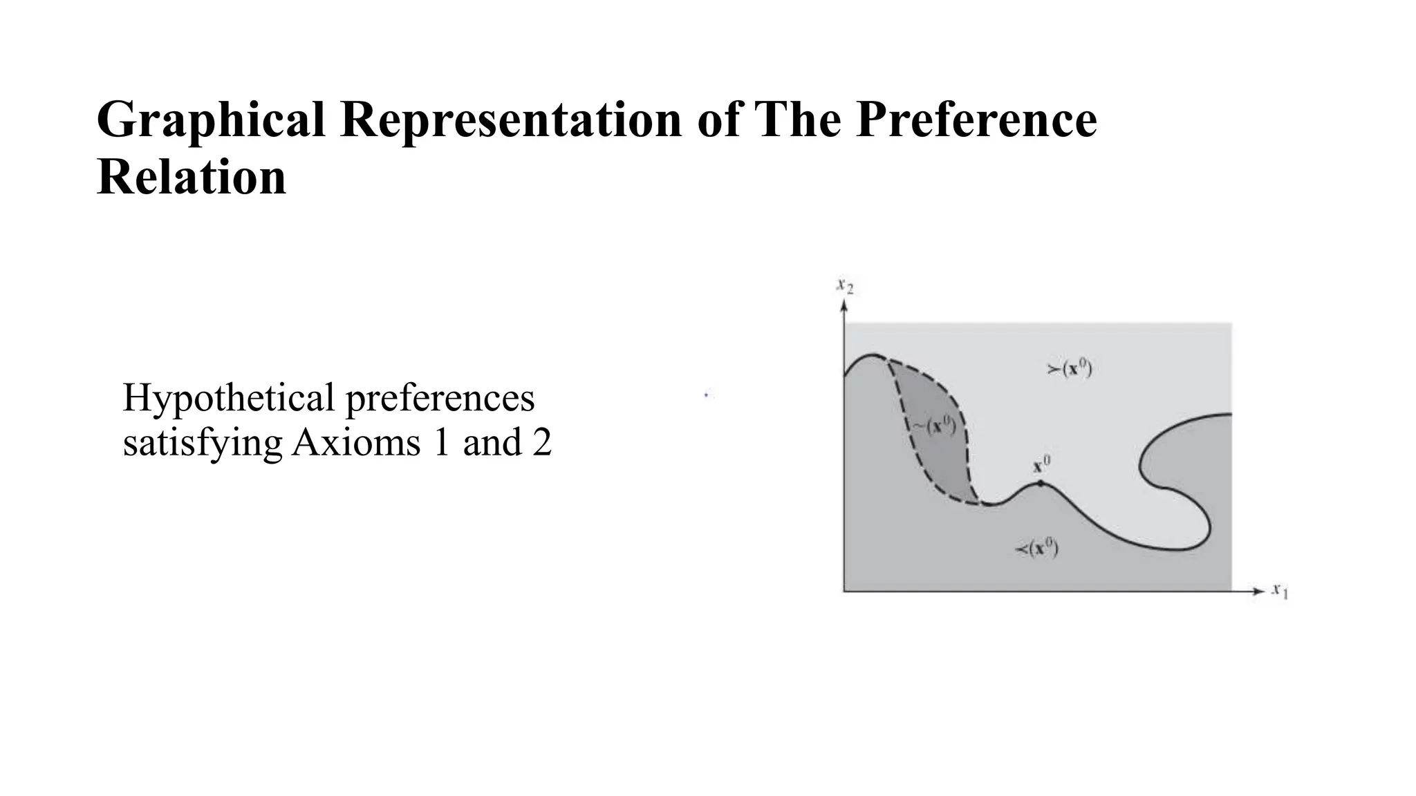
The document discusses consumer preference relations and utility theory. It defines consumer preference as a binary relation on a consumption set. It then lists six axioms that consumer preference relations must satisfy: completeness, transitivity, continuity, local nonsatiation, strict monotonicity, and convexity. It shows how preferences that satisfy these axioms can be represented by a continuous utility function. It also discusses properties of indirect utility functions and expenditure functions.

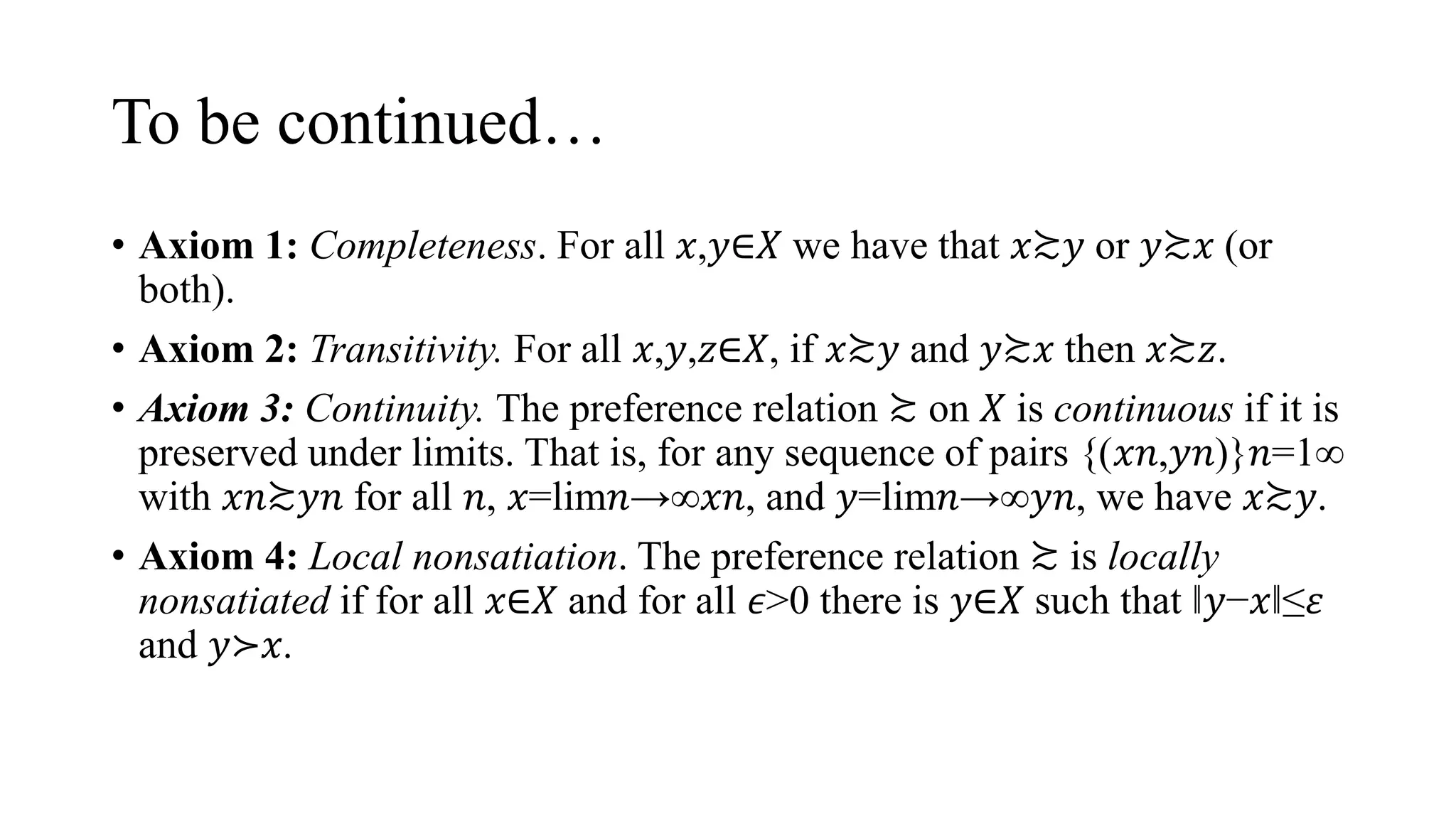
![To be continued…
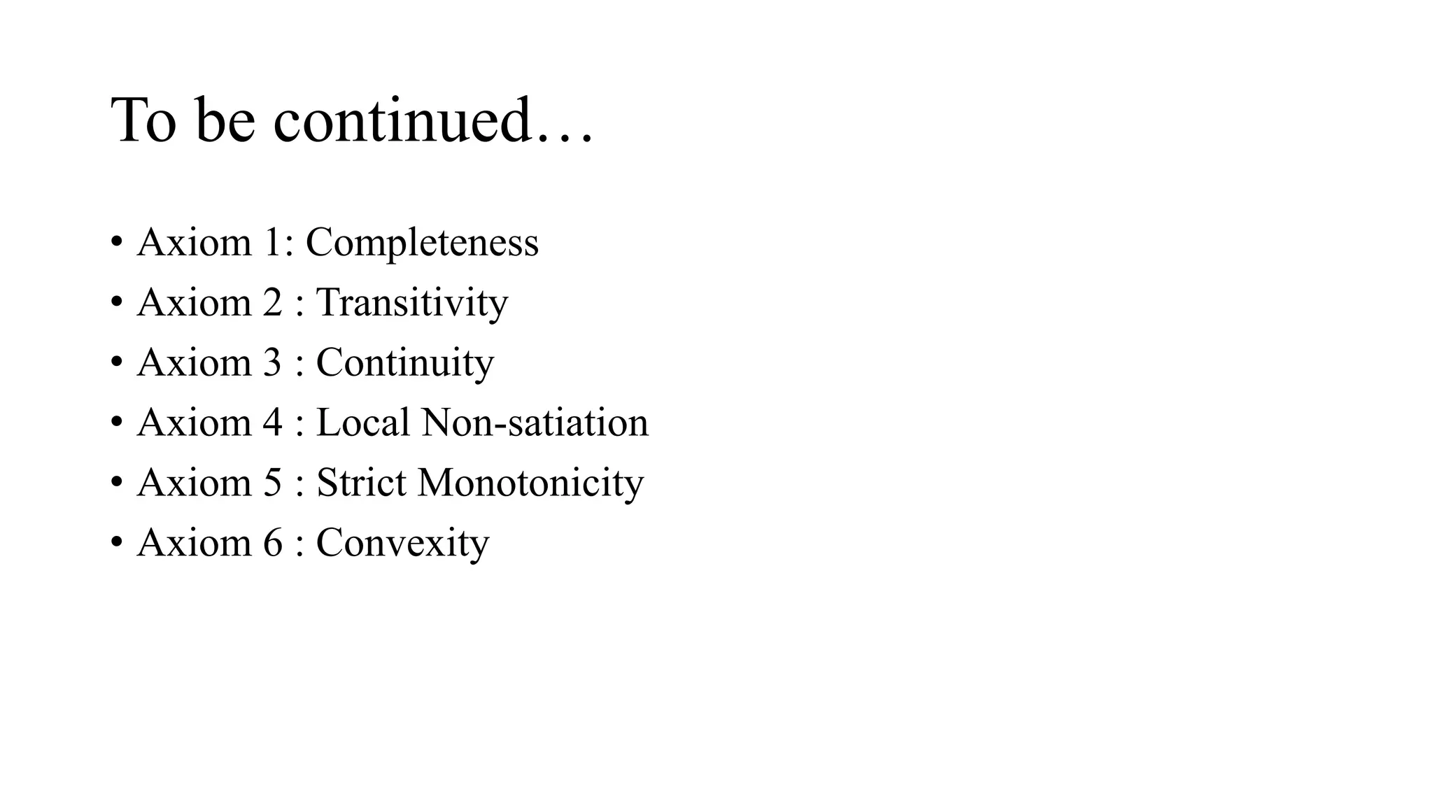
• Axiom 5: Strict monotonicity. The preference relation ≿ on 𝑋 is
monotone if for all 𝑥,𝑦∈ℝ+𝑛, 𝑥≥𝑦 implies 𝑥≿𝑦. It is strongly
monotone if 𝑥≫𝑦 implies 𝑥≻𝑦.
• Axiom 6: Convexity. The preference relation ≿ is convex if for every 𝑥
,𝑦,𝑧∈𝑋, the superior set (𝑦∈ℝ+𝑛∶𝑦≿𝑥) is convex. If, 𝑦≿𝑥 and 𝑧≿𝑥,
then 𝑡𝑦+(1 – 𝑡)𝑧≿𝑥, for all 𝑡∈[0,1]. Strict convexity implies that for
every 𝑥,𝑦≠𝑧∈𝑋, if 𝑦≿𝑥 and 𝑧≿𝑥, then 𝑡𝑦+(1 – 𝑡)𝑧≻𝑥, for all 𝑡∈(0,1).](https://image.slidesharecdn.com/chapter1ppt-220728181025-405ed7fc/75/CHAPTER-1-PPT-pptx-4-2048.jpg)


![αe Z for all nonnegative scalars α≥0. If α=1, then αe=(1,….,1) coincides with e. if
α>1, the point αe lies further out from the origin than e. for 0<α<1, the point αe
lies between the origin and e. for every x monotonicity implies that x.
Also for any such that ex, we have ex. monotonicity and continuity can then be
shown to imply that there is a unique value α(x)[0,α] such that α(x)e. By
continuity, the upper and lower contour sets of x are closed. Hence, the sets
A={α and B={ α arenonempty and closed.
By completeness of The nonemptyness and closedness of A and B, along with
the fact that is connected, imply that A Thus there exist a scalar αsuch that αe.](https://image.slidesharecdn.com/chapter1ppt-220728181025-405ed7fc/75/CHAPTER-1-PPT-pptx-16-2048.jpg)


![• To proof 2, We must show that v (p,y) = v (tp,ty) for
all t > 0.
•
• v(tp,ty) =[max u(x) s.t. tp·x ≤ ty], which is
equivalent to [max u(x) s.t. p·x ≤ y] because we may
divide both sides of the constraint by t > 0 without
affecting the set of bundles satisfying it.
• Now , v(tp,ty) =[max u(x) s.t. p·x ≤ y]=v(p,y).
• s.𝑡. 𝒑.𝑥 ≤ 𝑦
•](https://image.slidesharecdn.com/chapter1ppt-220728181025-405ed7fc/75/CHAPTER-1-PPT-pptx-30-2048.jpg)


![• Proof: Because u(·) is strictly increasing on ,
it attains a minimum at x = 0, but does not
attain a maximum. Moreover, because u(·) is
continuous, the set U of attainable utility
numbers must be an interval. Consequently, U
= [u(0), u¯)] for u¯ > u(0), and where u¯ may
be either finite or +∞.](https://image.slidesharecdn.com/chapter1ppt-220728181025-405ed7fc/75/CHAPTER-1-PPT-pptx-60-2048.jpg)
![• To prove 2, fix (p, u) ∈ × [u(0), u¯]. now, v(p, e(p,
u)) ≥ u. Again, to show that this must be an equality,
suppose to the contrary that v(p, e(p, u)) > u. There
are two cases to consider: u = u(0) and u > u(0). We
shall consider the second case only, leaving the first
as an exercise. Letting y = e(p, u), we then have v(p,
y) > u. Now, because e(p, u(0)) = 0 and because e(·) is
strictly increasing in utility by properties of the
expenditure function, y = e(p, u) > 0. Because v(·) is
continuous by properties of the utility function, we
may choose ε > 0 small enough so that y − ε > 0 and
v(p, y − ε) > u. Thus, income y − ε is sufficient, at
prices p, to achieve utility greater than u. Hence, we
must have e(p, u) ≤ y − ε. But this contradicts the fact
that y = e(p, u).](https://image.slidesharecdn.com/chapter1ppt-220728181025-405ed7fc/75/CHAPTER-1-PPT-pptx-61-2048.jpg)


![Introduction
Agriculture of Bangladesh:
• Comprises about 15.33% of the country’s GDP.
• Employs around 45% of the total labour force. [BBS,2016].
Bangladesh’s energy crisis and irrigation:
Irrigation is defined as a system that distributes water to targeted area.
Irrigation sector in Bangladesh suffers due to the countywide electricity crisis. Energy
infrastructure is quite small, inefficient, and poorly managed.
Solar power irrigation system brings a clean & simple alternative to the conventional fuel fired
engine or grid electricity driven pump in this regard to resolve the issue.
Solar Powered Irrigation System :
Using submergible pumps, PV cells are used to generate electricity , which is stored in
rechargeable batteries. Then current is passed by wire to DC pump which collects water and store
to reserve tank. Then water is passed to narrow canal to crops land.](https://image.slidesharecdn.com/chapter1ppt-220728181025-405ed7fc/75/CHAPTER-1-PPT-pptx-94-2048.jpg)
![Previous Study :
The number of published paper regarding solar irrigation plant in Bangladesh is very few as this
concept is quite new in the country.
Solar power generated electricity is environmentally feasible & ample opportunity in Bangladesh
& top priority in the 21st century. [Khalequzzaman,2007].
Off-grid water pumping by using solar energy is a viable option. [ Odeh et. al ,2009] .
Average annual sunlight hours in Bangladesh compared with other DCs like Germany & Spain ,
notable for development in solar energy sector. [ Shakir, Rahman, & Shahadat, 2012] .
Research Methodology :
• Qualitative statistical analysis using primary data.
• Secondary data were collected from Bangladesh Bank websites.
• NPV , IRR, & simple Payback period were investigated to determine the economic
feasibility of the project .](https://image.slidesharecdn.com/chapter1ppt-220728181025-405ed7fc/75/CHAPTER-1-PPT-pptx-95-2048.jpg)
![Data Analysis and Findings
Present irrigation scenario in Bangladesh [ Roy,2016]
Irrigation pumps run by electricity :
Total : 0.27 ml pumps
Area coverage : 1.7 ml hectares of land
Electricity consumption : 1500 MW.
Irrigation pumps run by diesel :
Total :1.34 ml pumps
Area coverage : 3.4 ml hectares of land
Fuel consumption : 1 ml tons diesel/ year worth $900 ml
Subsidy : $ 280 ml .](https://image.slidesharecdn.com/chapter1ppt-220728181025-405ed7fc/75/CHAPTER-1-PPT-pptx-96-2048.jpg)
![Solar Pump Implementation Status :
Approved : 241 pumps
Installed : 108 pumps
Under consideration : 133 pumps
Target : 50,000 by 2025 [ PDB]
Funding sources : Grant : IDCOL,BCCRF, ADB, USAID.
: Loan : IDA , JICA.
How Solar Water Pump Works : [ www.economicsdiscussions.com ]](https://image.slidesharecdn.com/chapter1ppt-220728181025-405ed7fc/75/CHAPTER-1-PPT-pptx-97-2048.jpg)
![How Solar Water Pumps works : [ www.economicsdiscussions.com ]](https://image.slidesharecdn.com/chapter1ppt-220728181025-405ed7fc/75/CHAPTER-1-PPT-pptx-98-2048.jpg)
![Cost analysis : [ Roy,2016 ]](https://image.slidesharecdn.com/chapter1ppt-220728181025-405ed7fc/75/CHAPTER-1-PPT-pptx-99-2048.jpg)
![Financial Structure
Sample of an 11 kwp solar water pump [BPDB-website,nov.2016]](https://image.slidesharecdn.com/chapter1ppt-220728181025-405ed7fc/75/CHAPTER-1-PPT-pptx-100-2048.jpg)
![Advantages of Solar water pump
The production of power is environment friendly,
No fuel cost is involved & lower maintenance cost,
Solar PV systems are durable,
No noise pollution is generated ,etc.
Why replace Diesel with Solar Pumps :
Frequent technical problems & high maintenance costs for diesel pumps.
Increasing cost of diesel & on-going subsidy burden on government.
Transportation of diesel to the field is challenging.
CO2 Emission in equivalent system : [ Ahammed ,2008]
Parameter Unit Value
solar energy kg/day 0
grid electricity kg/day 2566.24
diesel fuel kg/day 42.88](https://image.slidesharecdn.com/chapter1ppt-220728181025-405ed7fc/75/CHAPTER-1-PPT-pptx-101-2048.jpg)
![Challenges of Solar system :
High installation cost ,
Long installation time ,
Limited use ,
The water yield of the solar pump varies according to sunlight.
Which have major impact on potentiality of using solar energy for irrigation.
Policy Recommendations :
Social awareness focusing on the sustainable use of solar power plant.
Authority can encourage citizens announcing particular percentage of tax redemption to those
who installs solar pump. [Hoque ,2016 ].
Role of Government :
Proper regulations & subsidies should be implemented by GOB to successfully expand solar
powered irrigation system .](https://image.slidesharecdn.com/chapter1ppt-220728181025-405ed7fc/75/CHAPTER-1-PPT-pptx-102-2048.jpg)