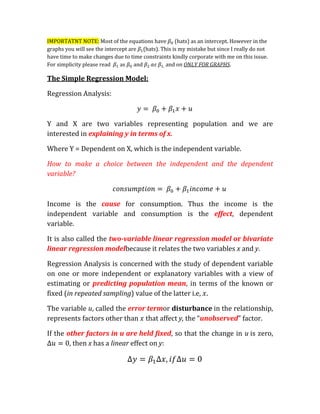
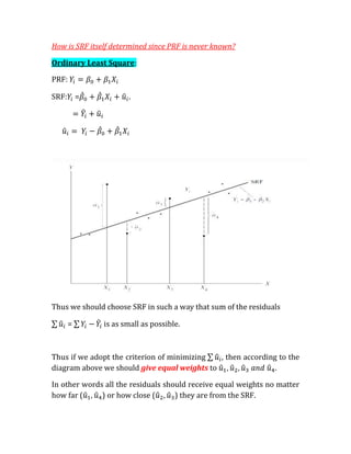
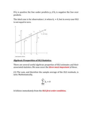
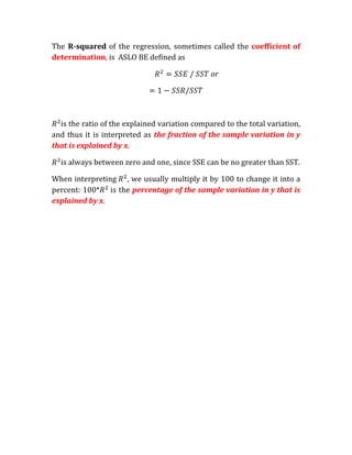
IMPORTATNT NOTE: Most of the equations have (hats) as an intercept. However in the
graphs you will see the intercept are (hats). This is my mistake but since I really do not
have time to make changes due to time constraints kindly corporate with me on this issue.
For simplicity please read    as and            and on ONLY FOR GRAPHS.

The Simple Regression Model:

Regression Analysis:


Y and X are two variables representing population and we are
interested in explaining y in terms of x.

Where Y = Dependent on X, which is the independent variable.

How to make a choice between the independent and the dependent
variable?


Income is the cause for consumption. Thus the income is the
independent variable and consumption is the effect, dependent
variable.

It is also called the two-variable linear regression model or bivariate
linear regression modelbecause it relates the two variables x and y.

Regression Analysis is concerned with the study of dependent variable
on one or more independent or explanatory variables with a view of
estimating or predicting population mean, in terms of the known or
fixed (in repeated sampling) value of the latter i.e,

The variable u, called the error termor disturbance in the relationship,
represents factors other than that affect y, the “unobserved” factor.

If the other factors in u are held fixed, so that the change in u is zero,
        , then x has a linear effect on y:
Thus, the change in y is simply      multiplied by the change in x.

Terminology- Notation:

Dependent Variable Independent Variable
  Explained Variable                       Explanatory Variable
  Predicted                                         Predicator
  RegressandRegressor
  Response                                           Stimulus
  Endogenous                                          Exogeneous
  Outcome                                            Covariate
  Controlled                                         Control Variables

          are two unknown but fixed parameters known as the
regression coefficients.

Eg: Suppose in a "total Population" we have 60 families living in a
community called XYZ and their weekly income (X) and weekly
consumption (Y) are both in dollars.
    X         80   100   120   140 160 180     200 220       240  260
    Y          55   65    79    80 102 110     120 135       137 150
               60   70    84    93 107 115     136 137       145 152
               65   74    90    95 110 120     140 140       155 175
               70   80    94   103 116 130     144 152       165 178
               75   85    98   108 118 135     145 157       175 180
                 0  88     0   113 125 140       0 160       189 185
                 0   0     0   115   0   0       0 162         0 191
Total         325 462    445   707 678 750     685 1043      966 1211
Conditional
Means of
Y, E(Y/X)      65   77    89   101   113   125 137     149   161   173


The 60 families of X are divided into 10 income groups from $80-$260.

The values of X are "fixed" and 10 Y subpopulation.

There is a considerable variation in each income group
Geometrically, then a population regression curve is simply the locus of
the conditional means of the dependent variable for the fixed values
of the explanatory variable (s).


The conditional mean

Where          denotes some function of the explanatory variable X.

E(Y/ ) is a linear function of      say of a type:

E         =


Meaning of term Liner:

    1. Liner in Variables i.e. X i.e. E(Y/              is not Liner.

    2. Liner in Parameters i.e.              .

    E         =             is not linear.
Eg: Linear in Parameters:


But for now whenever we refer to the term "linear" regression we only
mean linear in parameters the

Two way scatter plot of income and consumption


                                                                   Population
                                                                   Regression
                                                                   Line
The Population Regression Line passes between the "Average" values
of consumption E(Y/X) which is also known as the conditional
expected value.

The CEV tells us the expected value of weekly consumption expenditure
or a family whose income is $80, $100…

Unconditional Expected Value: The unconditional expected value of
weekly consumption expenditure is given by E(Y) it disregards the
income levels of various families.

E(Y) = 7272/60 = $121.20

It tells us the expected value of weekly consumption expenditure of
"any" family.

Thus;

Conditional mean E(Y/X) is a function of             where     =      ,
         and so on.

It is a liner function, AND is also known asthe conditional Expected
Function, Population Regression Function or Population Function.

E        =

Where              are two unknown but fixed parameters known as
the regression coefficients.

And     is the intercept and   is the slope.

The main objective of the regression analysis is to estimate the values
of the unknown's           on the basis of observations Y and X.

We saw previously that as family's income increases, family's
consumption expenditure on average increases too.

But what about the individual family?
For example see that as income increases from $80 to $100 we see
particular families consumption is $65, which is less than consumption
expenditure of two families whose weekly income is $ 80.

Thus we express this deviation of an individual   as:

                or             ) or

                                                                 .

The expenditure of an individual family given its income level can be
expressed as:

      1. E      = Systematic or deterministic and
      2.   = Nonsystematic and cannot be determined


       =


Taking the expected value on both sides:


           /   )+     /   ).


Before we make any assumption of u and x. We make an important
assumption i.e. as long as we include the intercept in the equation;
nothing is lost by assuming that the average value of u in the
"population" is zero.i.e. E(u) = 0.


Relationship between u and x:

We assume u and x are not correlated or u and x are not linearly related.
It is possible for u to be uncorrelated with x while being correlated with
the functions of x such as the .

Thus the better assumption involves that the expected value of u given
x is zero or E ( / = E(u) = 0.

This is called the zero conditional mean assumption.

The sample regression function:

So far we have only talked about the population of Y values
corresponding to the fixed X's.

When collecting data it is almost impossible to collect data on the entire
population.

Thus for most practical situations we have is a sample of Y values
corresponding to some fixed X's.

Thus our task is to estimate PRF based on the sample information.
OR;

                Where;            is   the    estimator    of        and
                      .

Thenumerical value obtained by the estimator is known as the
"Estimate".

Expressing SRF is stochastic term can be written as:

                    .

Where     is the residual term.

Conceptually    is analogus to     and can be regarded as the estimate of
  .

So far:

PRF:                and

SRF:


In terms of SRF:


In terms of PRF:
            )+

It is almost impossible for SRF and PRF to be the same due to sampling
problems thus our main objective is to choose                so that it
replicates           as close as possible.
How is SRF itself determined since PRF is never known?

Ordinary Least Square:

PRF:

SRF: =                .


Thus we should choose SRF in such a way that sum of the residuals

    =          is as small as possible.


Thus if we adopt the criterion of minimizing  , then according to the
diagram above we should give equal weights to

In other words all the residuals should receive equal weights no matter
how far (     ) or how close (      ) they are from the SRF.
And such a minimization is possible by adopting least square criteria
which states that SRF can be fixed in such a way that


   is as small as possible where;

                                                               .

   Thus our goal is to choose            in such a way that        is as
   small as possible which is done by OLS.

   Let                   =

   So we want to minimize                                  .

   Taking partial derivative with respect to           .

         = -2                                  .

         = -2                                      .


    =

                                           .

Plugging the values of

         ( -( -     )-       )=0

Upon rearranging gives:
( - )=            -


             - )( -        –


Provided that

   Thus

                               =               or


  equals the population covariance divided by the variance of
when                           .

Which concludes:

        If   and   are positively correlated then     is positive and
        If   and   are negatively correlated then      is negative.

Fitted Value and Residuals:

We assume that the intercept and slope                  , have been obtained
for a given sample of data.

Given              , we can obtain the fitted value   for each observation.

By definition each fitted value is on the OLS line.

The OLS residuals associated with observation i,            is the difference
between and the its fitted value.
If is positive the line under predicts        if   is negative the line over
predicts.

The ideal case is for observation   is when          , but in every case OLS
is not equal to zero.


Algebraic Prosperities of OLS Statistics:

There are several useful algebraic properties of OLS estimates and their
associated statistics. We now cover the three most important of these.

(1) The sum, and therefore the sample average of the OLS residuals, is
zero. Mathematically,


It follows immediately from the OLS first order condition.
This means OLS estimates             are chosen to make the residuals
add up to zero (for any data set). This says nothing about the residual
for any particular observation

(2) The sample covariance between the regressor and the OLS residuals
is zero. This can be written as:


The sample average of the OLS residuals is zero.

Example:


Thus                     and u captures all the factors not included in the
model eg: aptitude, ability as so on.

(3) The point (      is always on the OLS regression line.

Writing each as its fitted value, plus its residual, provides another way
to interpret an OLS regression.

For each i, write:            .
From property (1) above, the average of the residuals is zero;
equivalently, the sample average of the fitted values, , is the same as
the sample average of the   , or = .

Further, properties (1) and (2) can be used to show that the sample
covariance between             is zero.

Thus, we can view OLS as decomposing each       into two parts, a fitted
value and a residual.

The fitted values and residuals are uncorrelated in the sample.


Precision Or Standard Errors of Least Square Estimates:

Thus far we know that least square estimates are functions of SAMPLE
data.

And our estimates             will change with each change in sample.

Therefore a proper measure of reliability and precision is needed. And
such precision/ reliability is measured by STANDARD ERROR.

Define the total sum of squares (SST), the explained sum of squares
(SSE), and the residual sum of squares (SSR) (also known as the sum
of squared residuals), as follows:

SST =
SSE =

SSR =               .
SST is a measure of the total sample variation in the ; that is, it
measures how spread out the is in the sample.

If we divide SST by n-1 we obtain the sample variance of y.
Similarly, SSE measures the sample variation in the    (where we use the
fact that       ), and

SSR measures the sample variation in the .

The total variation in y can always be expressed as the sum of the
explained variation and the unexplained variation SSR. Thus,

                          SST = SSE +SSR.
PROOF:


Since the covariance between the residuals and the fitted value is zero.
We have

                         SST = SSE +SSR.


Goodness of Fit:

So far, we have no way of measuring how well the explanatory or
independent variable, x, explains the dependent variable, y.

It is often useful to compute a number that summarizes how well the
OLS regression line fits the data.

Assuming that the total sum of squares, SST, is not equal to zero—which
is true except in the very unlikely event that all the equal the same
value—we can divide SST on both sides to obtain:


Alternatively:
The R-squared of the regression, sometimes called the coefficient of
determination, is ASLO BE defined as

                                               or


  is the ratio of the explained variation compared to the total variation,
and thus it is interpreted as the fraction of the sample variation in y
that is explained by x.

  is always between zero and one, since SSE can be no greater than SST.

When interpreting , we usually multiply it by 100 to change it into a
percent: 100* is the percentage of the sample variation in y that is
explained by x.

2.1 the simple regression model

  • 1.
    IMPORTATNT NOTE: Mostof the equations have (hats) as an intercept. However in the graphs you will see the intercept are (hats). This is my mistake but since I really do not have time to make changes due to time constraints kindly corporate with me on this issue. For simplicity please read as and and on ONLY FOR GRAPHS. The Simple Regression Model: Regression Analysis: Y and X are two variables representing population and we are interested in explaining y in terms of x. Where Y = Dependent on X, which is the independent variable. How to make a choice between the independent and the dependent variable? Income is the cause for consumption. Thus the income is the independent variable and consumption is the effect, dependent variable. It is also called the two-variable linear regression model or bivariate linear regression modelbecause it relates the two variables x and y. Regression Analysis is concerned with the study of dependent variable on one or more independent or explanatory variables with a view of estimating or predicting population mean, in terms of the known or fixed (in repeated sampling) value of the latter i.e, The variable u, called the error termor disturbance in the relationship, represents factors other than that affect y, the “unobserved” factor. If the other factors in u are held fixed, so that the change in u is zero, , then x has a linear effect on y:
  • 2.
    Thus, the changein y is simply multiplied by the change in x. Terminology- Notation: Dependent Variable Independent Variable Explained Variable Explanatory Variable Predicted Predicator RegressandRegressor Response Stimulus Endogenous Exogeneous Outcome Covariate Controlled Control Variables are two unknown but fixed parameters known as the regression coefficients. Eg: Suppose in a "total Population" we have 60 families living in a community called XYZ and their weekly income (X) and weekly consumption (Y) are both in dollars. X 80 100 120 140 160 180 200 220 240 260 Y 55 65 79 80 102 110 120 135 137 150 60 70 84 93 107 115 136 137 145 152 65 74 90 95 110 120 140 140 155 175 70 80 94 103 116 130 144 152 165 178 75 85 98 108 118 135 145 157 175 180 0 88 0 113 125 140 0 160 189 185 0 0 0 115 0 0 0 162 0 191 Total 325 462 445 707 678 750 685 1043 966 1211 Conditional Means of Y, E(Y/X) 65 77 89 101 113 125 137 149 161 173 The 60 families of X are divided into 10 income groups from $80-$260. The values of X are "fixed" and 10 Y subpopulation. There is a considerable variation in each income group
  • 3.
    Geometrically, then apopulation regression curve is simply the locus of the conditional means of the dependent variable for the fixed values of the explanatory variable (s). The conditional mean Where denotes some function of the explanatory variable X. E(Y/ ) is a linear function of say of a type: E = Meaning of term Liner: 1. Liner in Variables i.e. X i.e. E(Y/ is not Liner. 2. Liner in Parameters i.e. . E = is not linear.
  • 4.
    Eg: Linear inParameters: But for now whenever we refer to the term "linear" regression we only mean linear in parameters the Two way scatter plot of income and consumption Population Regression Line
  • 5.
    The Population RegressionLine passes between the "Average" values of consumption E(Y/X) which is also known as the conditional expected value. The CEV tells us the expected value of weekly consumption expenditure or a family whose income is $80, $100… Unconditional Expected Value: The unconditional expected value of weekly consumption expenditure is given by E(Y) it disregards the income levels of various families. E(Y) = 7272/60 = $121.20 It tells us the expected value of weekly consumption expenditure of "any" family. Thus; Conditional mean E(Y/X) is a function of where = , and so on. It is a liner function, AND is also known asthe conditional Expected Function, Population Regression Function or Population Function. E = Where are two unknown but fixed parameters known as the regression coefficients. And is the intercept and is the slope. The main objective of the regression analysis is to estimate the values of the unknown's on the basis of observations Y and X. We saw previously that as family's income increases, family's consumption expenditure on average increases too. But what about the individual family?
  • 6.
    For example seethat as income increases from $80 to $100 we see particular families consumption is $65, which is less than consumption expenditure of two families whose weekly income is $ 80. Thus we express this deviation of an individual as: or ) or . The expenditure of an individual family given its income level can be expressed as: 1. E = Systematic or deterministic and 2. = Nonsystematic and cannot be determined = Taking the expected value on both sides: / )+ / ). Before we make any assumption of u and x. We make an important assumption i.e. as long as we include the intercept in the equation; nothing is lost by assuming that the average value of u in the "population" is zero.i.e. E(u) = 0. Relationship between u and x: We assume u and x are not correlated or u and x are not linearly related.
  • 7.
    It is possiblefor u to be uncorrelated with x while being correlated with the functions of x such as the . Thus the better assumption involves that the expected value of u given x is zero or E ( / = E(u) = 0. This is called the zero conditional mean assumption. The sample regression function: So far we have only talked about the population of Y values corresponding to the fixed X's. When collecting data it is almost impossible to collect data on the entire population. Thus for most practical situations we have is a sample of Y values corresponding to some fixed X's. Thus our task is to estimate PRF based on the sample information.
  • 8.
    OR; Where; is the estimator of and . Thenumerical value obtained by the estimator is known as the "Estimate". Expressing SRF is stochastic term can be written as: . Where is the residual term. Conceptually is analogus to and can be regarded as the estimate of . So far: PRF: and SRF: In terms of SRF: In terms of PRF: )+ It is almost impossible for SRF and PRF to be the same due to sampling problems thus our main objective is to choose so that it replicates as close as possible.
  • 9.
    How is SRFitself determined since PRF is never known? Ordinary Least Square: PRF: SRF: = . Thus we should choose SRF in such a way that sum of the residuals = is as small as possible. Thus if we adopt the criterion of minimizing , then according to the diagram above we should give equal weights to In other words all the residuals should receive equal weights no matter how far ( ) or how close ( ) they are from the SRF.
  • 10.
    And such aminimization is possible by adopting least square criteria which states that SRF can be fixed in such a way that is as small as possible where; . Thus our goal is to choose in such a way that is as small as possible which is done by OLS. Let = So we want to minimize . Taking partial derivative with respect to . = -2 . = -2 . = . Plugging the values of ( -( - )- )=0 Upon rearranging gives:
  • 11.
    ( - )= - - )( - – Provided that Thus = or equals the population covariance divided by the variance of when . Which concludes: If and are positively correlated then is positive and If and are negatively correlated then is negative. Fitted Value and Residuals: We assume that the intercept and slope , have been obtained for a given sample of data. Given , we can obtain the fitted value for each observation. By definition each fitted value is on the OLS line. The OLS residuals associated with observation i, is the difference between and the its fitted value.
  • 12.
    If is positivethe line under predicts if is negative the line over predicts. The ideal case is for observation is when , but in every case OLS is not equal to zero. Algebraic Prosperities of OLS Statistics: There are several useful algebraic properties of OLS estimates and their associated statistics. We now cover the three most important of these. (1) The sum, and therefore the sample average of the OLS residuals, is zero. Mathematically, It follows immediately from the OLS first order condition.
  • 13.
    This means OLSestimates are chosen to make the residuals add up to zero (for any data set). This says nothing about the residual for any particular observation (2) The sample covariance between the regressor and the OLS residuals is zero. This can be written as: The sample average of the OLS residuals is zero. Example: Thus and u captures all the factors not included in the model eg: aptitude, ability as so on. (3) The point ( is always on the OLS regression line. Writing each as its fitted value, plus its residual, provides another way to interpret an OLS regression. For each i, write: .
  • 14.
    From property (1)above, the average of the residuals is zero; equivalently, the sample average of the fitted values, , is the same as the sample average of the , or = . Further, properties (1) and (2) can be used to show that the sample covariance between is zero. Thus, we can view OLS as decomposing each into two parts, a fitted value and a residual. The fitted values and residuals are uncorrelated in the sample. Precision Or Standard Errors of Least Square Estimates: Thus far we know that least square estimates are functions of SAMPLE data. And our estimates will change with each change in sample. Therefore a proper measure of reliability and precision is needed. And such precision/ reliability is measured by STANDARD ERROR. Define the total sum of squares (SST), the explained sum of squares (SSE), and the residual sum of squares (SSR) (also known as the sum of squared residuals), as follows: SST = SSE = SSR = . SST is a measure of the total sample variation in the ; that is, it measures how spread out the is in the sample. If we divide SST by n-1 we obtain the sample variance of y.
  • 15.
    Similarly, SSE measuresthe sample variation in the (where we use the fact that ), and SSR measures the sample variation in the . The total variation in y can always be expressed as the sum of the explained variation and the unexplained variation SSR. Thus, SST = SSE +SSR. PROOF: Since the covariance between the residuals and the fitted value is zero.
  • 16.
    We have SST = SSE +SSR. Goodness of Fit: So far, we have no way of measuring how well the explanatory or independent variable, x, explains the dependent variable, y. It is often useful to compute a number that summarizes how well the OLS regression line fits the data. Assuming that the total sum of squares, SST, is not equal to zero—which is true except in the very unlikely event that all the equal the same value—we can divide SST on both sides to obtain: Alternatively:
  • 17.
    The R-squared ofthe regression, sometimes called the coefficient of determination, is ASLO BE defined as or is the ratio of the explained variation compared to the total variation, and thus it is interpreted as the fraction of the sample variation in y that is explained by x. is always between zero and one, since SSE can be no greater than SST. When interpreting , we usually multiply it by 100 to change it into a percent: 100* is the percentage of the sample variation in y that is explained by x.