Econometrics ch6

1. 405405 ECONOMETRICSECONOMETRICS
Chapter # 5:Chapter # 5: TWO-VARIABLE REGRESSION:TWO-VARIABLE REGRESSION:
INTERVAL ESTIMATION AND HYPOTHESIS TESTINGINTERVAL ESTIMATION AND HYPOTHESIS TESTING
Domodar N. GujaratiDomodar N. Gujarati
Prof. M. El-SakkaProf. M. El-Sakka
Dept of Economics. Kuwait UniversityDept of Economics. Kuwait University

2. Introduction
• The theory of estimation consists of two parts:The theory of estimation consists of two parts: point estimationpoint estimation andand intervalinterval
estimation.estimation. We have discussed point estimation thoroughly in the previousWe have discussed point estimation thoroughly in the previous
two chapters. In this chapter we first consider interval estimation and thentwo chapters. In this chapter we first consider interval estimation and then
take up the topic of hypothesis testing, a topic related to interval estimation.take up the topic of hypothesis testing, a topic related to interval estimation.

3. INTERVAL ESTIMATION: SOME BASIC IDEAS
• Look at the estimated MPC inLook at the estimated MPC in YˆYˆii = 24.4545 + 0.5091X= 24.4545 + 0.5091Xii ,, which is a singlewhich is a single
(point) estimate(point) estimate of the unknown populationof the unknown population MPCMPC ββ22.. How reliable is thisHow reliable is this
estimate? A single estimate is likely to differ from the true value, althoughestimate? A single estimate is likely to differ from the true value, although
inin repeated sampling its mean value is expected to be equal to the true value.repeated sampling its mean value is expected to be equal to the true value.
• InIn statistics the reliabilitystatistics the reliability of a point estimator is measuredof a point estimator is measured by its standardby its standard
errorerror. Therefore, we may. Therefore, we may construct an interval around the point estimatorconstruct an interval around the point estimator,,
say within two or three standard errorssay within two or three standard errors on either sideon either side of the point estimator,of the point estimator,
such that this interval has, say, 95 percent probability of including the truesuch that this interval has, say, 95 percent probability of including the true
parameter value.parameter value.
• Assume that we want to find out how “close” is, say,Assume that we want to find out how “close” is, say, βˆβˆ22 to βto β22.. We try to findWe try to find
out two positive numbersout two positive numbers δ and αδ and α,, the latter lying betweenthe latter lying between 0 and 10 and 1, such, such
that the probability that the random intervalthat the probability that the random interval ((βˆβˆ22 − δ, βˆ− δ, βˆ22 + δ)+ δ) contains thecontains the
true βtrue β22 isis 1 − α1 − α. Symbolically,. Symbolically,
• Pr (Pr (βˆβˆ22 − δ ≤ β− δ ≤ β22 ≤ βˆ≤ βˆ22 + δ) = 1 − α+ δ) = 1 − α (5.2.1)(5.2.1)
• Such an interval, if it exists, is known as a confidence interval.Such an interval, if it exists, is known as a confidence interval.

4. • 1 −1 − αα isis known as theknown as the confidence coefficientconfidence coefficient; and; and
• α (0 < α < 1)α (0 < α < 1) is known as theis known as the levellevel of significanceof significance..
• The endpoints of the confidence interval are known as theThe endpoints of the confidence interval are known as the confidence limitsconfidence limits
(also known as critical values(also known as critical values),), βˆβˆ22 − δ− δ being thebeing the lowerlower confidence limit andconfidence limit and
βˆβˆ22 + δ+ δ thethe upperupper confidence limitconfidence limit..
• IfIf α = 0.05, or 5 percent, (5.2.1) would read: Theα = 0.05, or 5 percent, (5.2.1) would read: The probability that theprobability that the
(random)(random) interval shown there includes the trueinterval shown there includes the true ββ22 isis 0.950.95, or 95 percent., or 95 percent.
The interval estimator thus gives aThe interval estimator thus gives a range of valuesrange of values within which thewithin which the truetrue ββ22
may lie.may lie.

5. • It is very important to know the following aspects of interval estimation:It is very important to know the following aspects of interval estimation:
• 1. Equation (5.2.1) does not say that the probability of1. Equation (5.2.1) does not say that the probability of ββ22 lying betweenlying between thethe
given limits isgiven limits is 1 −1 − αα.. What (5.2.1) states is that the probability ofWhat (5.2.1) states is that the probability of
constructing an intervalconstructing an interval that containsthat contains ββ22 isis 1 − α1 − α..
• 2. The interval (5.2.1) is2. The interval (5.2.1) is a random intervala random interval; that is, it will vary from one; that is, it will vary from one
sample to the next because it is based onsample to the next because it is based on βˆβˆ22, which is random., which is random.
• 3. (5.2.1) means: If in repeated sampling confidence intervals like it are3. (5.2.1) means: If in repeated sampling confidence intervals like it are
constructed a great many times on the 1 −constructed a great many times on the 1 − αα probability basis, then, in theprobability basis, then, in the
long run, on the average,long run, on the average, such intervals will enclose in 1 − α of the cases thesuch intervals will enclose in 1 − α of the cases the
true value of the parametertrue value of the parameter..
• 4. The interval (5.2.1) is random so long as4. The interval (5.2.1) is random so long as βˆβˆ22 is not knownis not known.. OnceOnce βˆβˆ22 isis
known,known, the interval (5.2.1) is no longer randomthe interval (5.2.1) is no longer random;; it isit is fixedfixed. In. In this situationthis situation
ββ22 is either in the fixed interval or outside itis either in the fixed interval or outside it. Therefore, the. Therefore, the probability isprobability is
either 1 or 0, if the 95% confidence interval were obtained as (0.4268 ≤either 1 or 0, if the 95% confidence interval were obtained as (0.4268 ≤ β2 ≤β2 ≤
0.5914), we cannot say the probability is 95%0.5914), we cannot say the probability is 95% that this interval includes thethat this interval includes the
truetrue ββ22. That probability is either 1 or 0.. That probability is either 1 or 0.

6. CONFIDENCE INTERVALS FOR REGRESSION
COEFFICIENTS β1 AND β2
• Confidence Interval forConfidence Interval for ββ22
• With the normality assumption forWith the normality assumption for uuii, the OLS estimators, the OLS estimators βˆβˆ11 and βˆand βˆ22 areare
themselvesthemselves normally distributednormally distributed with means and variances given therein.with means and variances given therein.
Therefore, for example, the VariableTherefore, for example, the Variable
• is a standardized normal variable. Therefore,is a standardized normal variable. Therefore, we can use the normalwe can use the normal
distribution to make probabilistic statements about βdistribution to make probabilistic statements about β22.. If σIf σ22
is known, anis known, an
important property of a normally distributed variable with meanimportant property of a normally distributed variable with mean μμ andand
variancevariance σσ22
is that the area under the normal curve betweenis that the area under the normal curve between μ ± σμ ± σ is aboutis about
68 percent68 percent,, that between the limitsthat between the limits μ ± 2σμ ± 2σ is about 95 percent, and thatis about 95 percent, and that
betweenbetween μ ± 3σμ ± 3σ is about 99.7 percent.is about 99.7 percent.

7. • ButBut σσ22
is rarely knownis rarely known, and in practice it is determined by the unbiased, and in practice it is determined by the unbiased
• estimatorestimator σσˆˆ22
. If we replace σ by σˆ, (5.3.1) may be written as:. If we replace σ by σˆ, (5.3.1) may be written as:
• where thewhere the se (se (βˆβˆ22)) now refers to the estimated standard error. Therefore,now refers to the estimated standard error. Therefore,
instead of using the normal distribution, we can use theinstead of using the normal distribution, we can use the t distributiont distribution toto
establish a confidence interval forestablish a confidence interval for ββ22 as follows:as follows:
• Pr (−Pr (−ttα/2α/2 ≤≤ t ≤ tt ≤ tα/2α/2) = 1 − α) = 1 − α (5.3.3)(5.3.3)
• wherewhere ttα/2α/2 is the value of theis the value of the tt variable obtained from thevariable obtained from the tt distribution fordistribution for α/2α/2
level of significancelevel of significance and n − 2 df;and n − 2 df; it is often called theit is often called the criticalcritical t valuet value atat α/2α/2 levellevel
of significance.of significance.

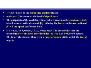
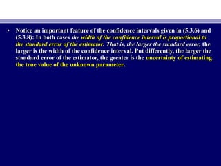
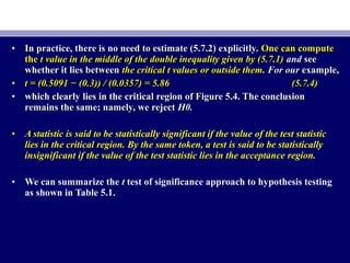
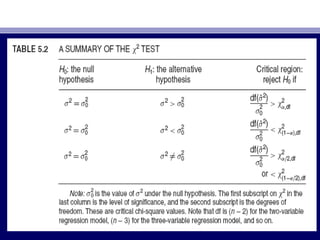
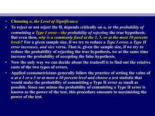
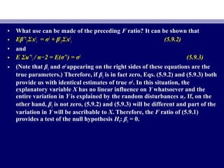
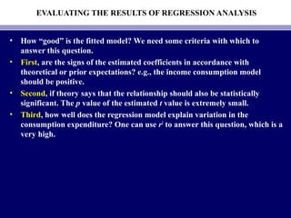
8. • Substitution of (5.3.2) into (5.3.3)Substitution of (5.3.2) into (5.3.3) YieldsYields
• Rearranging (5.3.4), we obtainRearranging (5.3.4), we obtain
• Pr [Pr [βˆβˆ22 −− tt α/2α/2 se (se (βˆβˆ22) ≤ β) ≤ β22 ≤ βˆ≤ βˆ22 ++ ttα/2α/2 se (se (βˆβˆ22)] = 1 − α)] = 1 − α (5.3.5)(5.3.5)
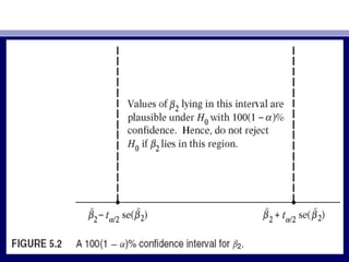
• Equation (5.3.5) provides a 100(1 −Equation (5.3.5) provides a 100(1 − α) percent confidence interval for βα) percent confidence interval for β22,,
which can be written more compactly aswhich can be written more compactly as
• 100(1 −100(1 − α)% confidence interval for βα)% confidence interval for β22::
• βˆβˆ22 ±± ttα/2α/2 se (se (βˆ2)βˆ2) (5.3.6)(5.3.6)
• Arguing analogously, and using (4.3.1) and (4.3.2), we can then write:Arguing analogously, and using (4.3.1) and (4.3.2), we can then write:
• Pr [Pr [βˆβˆ11 −− ttα/2α/2 se (se (βˆβˆ11) ≤ β) ≤ β11 ≤ βˆ≤ βˆ11 ++ ttα/2α/2 se (se (βˆβˆ11)] = 1 − α)] = 1 − α (5.3.7)(5.3.7)
• or, more compactly,or, more compactly,
• 100(1 −100(1 − α)% confidence interval for β1:α)% confidence interval for β1:
• βˆβˆ11 ±± ttα/2α/2 se (se (βˆβˆ11)) (5.3.8)(5.3.8)

9. • Notice an important feature of the confidence intervals given in (5.3.6) andNotice an important feature of the confidence intervals given in (5.3.6) and
(5.3.8): In both cases(5.3.8): In both cases thethe width of the confidence interval is proportional towidth of the confidence interval is proportional to
the standard error of the estimatorthe standard error of the estimator. That is, the larger the standard error,. That is, the larger the standard error, thethe
larger is the width of the confidence interval. Put differently, the larger thelarger is the width of the confidence interval. Put differently, the larger the
standard error of the estimator, the greater is thestandard error of the estimator, the greater is the uncertainty of estimatinguncertainty of estimating
the true value of the unknown parameterthe true value of the unknown parameter..

10. • We found thatWe found that βˆβˆ22 = 0.5091,= 0.5091, se (βˆse (βˆ22)) = 0.0357, and= 0.0357, and dfdf = 8. If we= 8. If we assumeassume αα ==
5%, that is, 95% confidence coefficient, then the5%, that is, 95% confidence coefficient, then the tt table showstable shows that for 8 df thethat for 8 df the
criticalcritical ttα/2α/2 == t0.025t0.025 = 2.306. Substituting these values in= 2.306. Substituting these values in (5.3.5), the 95%(5.3.5), the 95%
confidence interval forconfidence interval for ββ22 is asis as follows:follows:
• 00.4268 ≤ β.4268 ≤ β22 ≤ 0.5914≤ 0.5914 (5.3.9)(5.3.9)
• Or, using (5.3.6), it isOr, using (5.3.6), it is
• 00.5091 ± 2.306(0.0357).5091 ± 2.306(0.0357)
• that is,that is,
• 00.5091 ± 0.0823.5091 ± 0.0823 (5.3.10)(5.3.10)
• The interpretation of this confidence interval is: Given the confidenceThe interpretation of this confidence interval is: Given the confidence
coefficient of 95%, in 95 out of 100 cases intervals like (0.4268, 0.5914) willcoefficient of 95%, in 95 out of 100 cases intervals like (0.4268, 0.5914) will
contain the truecontain the true ββ22.. But,But, we cannot saywe cannot say that the probability is 95 percent thatthat the probability is 95 percent that
the specific interval (0.4268 to 0.5914) contains the truethe specific interval (0.4268 to 0.5914) contains the true ββ22 because thisbecause this
intervalinterval is now fixedis now fixed; therefore,; therefore, ββ22 either lies in it or does not.either lies in it or does not.

11. • Confidence Interval forConfidence Interval for β1β1
• Following (5.3.7), we can verify that the 95% confidence interval forFollowing (5.3.7), we can verify that the 95% confidence interval for ββ11 ofof
the consumption–income example isthe consumption–income example is
• 99.6643 ≤ β.6643 ≤ β11 ≤ 39.2448≤ 39.2448 (5.3.11)(5.3.11)
• Or, using (5.3.8), we find it isOr, using (5.3.8), we find it is
• 2424.4545 ± 2.306(6.4138).4545 ± 2.306(6.4138)
• that is,that is,
• 2424.4545 ± 14.7902.4545 ± 14.7902 (5.3.12)(5.3.12)
• In the long run, in 95 out of 100 cases intervals like (5.3.11) will contain theIn the long run, in 95 out of 100 cases intervals like (5.3.11) will contain the
truetrue ββ11; again the probability that this particular fixed interval includes the; again the probability that this particular fixed interval includes the
truetrue ββ11 is either 1 or 0.is either 1 or 0.

12. CONFIDENCE INTERVAL FOR σ2
• As pointed before, under the normality assumption, the variableAs pointed before, under the normality assumption, the variable
• χχ22
= (= (n− 2)n− 2) σσˆˆ22
//σσ22
(5.4.1)(5.4.1)
• follows thefollows the χχ22
distribution withdistribution with n − 2 dfn − 2 df. Therefore, we can use the. Therefore, we can use the χχ22
distributiondistribution to establish a confidence interval forto establish a confidence interval for σσ22
• Pr (Pr (χχ22
1−1−α/2α/2 ≤ χ≤ χ22
≤ χ≤ χ22
α/2α/2 )) = 1 − α= 1 − α (5.4.2)(5.4.2)
• WhereWhere χχ22
1−1−α/2α/2 andand χχ22
α/2α/2 are two critical values ofare two critical values of χχ22
obtainedobtained from the chi-squarefrom the chi-square
table fortable for n − 2 dfn − 2 df..
• SubstitutingSubstituting χχ22
from (5.4.1) into (5.4.2) and rearranging the terms, wefrom (5.4.1) into (5.4.2) and rearranging the terms, we obtainobtain
• which gives the 100(1 −which gives the 100(1 − α)% confidence interval for σα)% confidence interval for σ22
..

13. • To illustrate, weTo illustrate, we obtainobtain σσˆˆ22
= 42.1591= 42.1591 and df = 8. If α is chosen at 5 percent,and df = 8. If α is chosen at 5 percent,
the chi-square tablethe chi-square table for 8 df gives the following critical values:for 8 df gives the following critical values:
• χχ22
00.025.025 = 17.5346,= 17.5346, andand χχ22
00.975.975 = 2.1797.= 2.1797.
• These values show that the probability of a chi-square value exceedingThese values show that the probability of a chi-square value exceeding
17.534617.5346 is 2.5 percent and that ofis 2.5 percent and that of 2.17972.1797 isis 97.597.5 percent. Therefore, thepercent. Therefore, the
interval between these two values is the 95% confidence interval forinterval between these two values is the 95% confidence interval for χχ22
, as, as
shown diagrammatically in Figure 5.1.shown diagrammatically in Figure 5.1.
• Substituting the data of our example into (5.4.3 the 95% confidence intervalSubstituting the data of our example into (5.4.3 the 95% confidence interval
forfor σσ22
is as follows:is as follows:
• 1919.2347 ≤ σ.2347 ≤ σ22
≤ 154.7336≤ 154.7336 (5.4.4)(5.4.4)
• The interpretation of this interval is: If we establish 95% confidence limitsThe interpretation of this interval is: If we establish 95% confidence limits
onon σσ22
and if we maintain a priori that these limits will include true σand if we maintain a priori that these limits will include true σ22
,, we shallwe shall
be right in the long run 95 percent of the time.be right in the long run 95 percent of the time.

14. (Note the skewed characteristic of the chi-square distribution.)

15. HYPOTHESIS TESTING: THE CONFIDENCE-INTERVAL
APPROACH
• Two-Sided or Two-Tail TestTwo-Sided or Two-Tail Test
• To illustrate the confidence-interval approach,To illustrate the confidence-interval approach, look atlook at the consumption–the consumption–
income example, the estimated (MPC),income example, the estimated (MPC), βˆβˆ22, is 0.5091, is 0.5091. Suppose we postulate. Suppose we postulate
that:that:
• HH00:: ββ22 = 0.3= 0.3 and Hand H11:: ββ22 ≠≠ 0.30.3
• that is, the true MPC isthat is, the true MPC is 0.30.3 under the null hypothesisunder the null hypothesis but it is less than orbut it is less than or
greater thangreater than 0.30.3 under the alternative hypothesis. The alternative hypothesisunder the alternative hypothesis. The alternative hypothesis
is ais a two-sided hypothesistwo-sided hypothesis. It reflects the fact that. It reflects the fact that we do not have a strongwe do not have a strong
expectationexpectation about the direction in which the alternative hypothesis shouldabout the direction in which the alternative hypothesis should
move from the null hypothesis.move from the null hypothesis.
• Is the observedIs the observed βˆβˆ22 compatible with Hcompatible with H00? To answer this question, let us refer? To answer this question, let us refer toto
the confidence interval (5.3.9). We know that in the long run intervals likethe confidence interval (5.3.9). We know that in the long run intervals like
((0.4268, 0.59140.4268, 0.5914) will contain the true) will contain the true ββ22 with 95 percent probability.with 95 percent probability.

16. • Consequently,Consequently, in the long run such intervals provide a range or limits withinin the long run such intervals provide a range or limits within
which the truewhich the true ββ22 may lie with a confidence coefficientmay lie with a confidence coefficient of, say, 95%.of, say, 95%.
• Therefore, ifTherefore, if ββ22 underunder HH00 falls within the 100(1 − α)% confidencefalls within the 100(1 − α)% confidence interval,interval, wewe
do not reject the null hypothesisdo not reject the null hypothesis; if it lies outside the interval, we; if it lies outside the interval, we may rejectmay reject
itit. This range is illustrated schematically in Figure 5.2.. This range is illustrated schematically in Figure 5.2.
• Decision Rule: Construct a 100(1 − α)% confidence interval for βDecision Rule: Construct a 100(1 − α)% confidence interval for β22. If the β. If the β22
under Hunder H00 falls within this confidence interval, do not reject Hfalls within this confidence interval, do not reject H00, but if it falls, but if it falls
outside this interval, reject Houtside this interval, reject H00..
• Following this rule,Following this rule, HH00:: ββ22 = 0.3= 0.3 clearly liesclearly lies outside theoutside the 95%95% confidenceconfidence
interval given in (5.3.9). Therefore, we can reject the hypothesis that theinterval given in (5.3.9). Therefore, we can reject the hypothesis that the
true MPC istrue MPC is 0.30.3, with 95% confidence., with 95% confidence.

18. • In statistics, when we reject the null hypothesis, we say that our finding isIn statistics, when we reject the null hypothesis, we say that our finding is
statistically significantstatistically significant. On the other hand, when we do not reject the null. On the other hand, when we do not reject the null
hypothesis, we say that our finding ishypothesis, we say that our finding is not statistically significantnot statistically significant..
• One-Sided or One-Tail TestOne-Sided or One-Tail Test
• If we have a strong theoretical expectationIf we have a strong theoretical expectation that the alternative hypothesis isthat the alternative hypothesis is
one-sided or unidirectional rather than two-sided. Thus, for ourone-sided or unidirectional rather than two-sided. Thus, for our
consumption–income example, one could postulate thatconsumption–income example, one could postulate that
• HH00: β: β22 ≤ 0.3 and H≤ 0.3 and H11: β: β22 > 0.3> 0.3
• Perhaps economic theory or prior empirical work suggests that thePerhaps economic theory or prior empirical work suggests that the
marginal propensity to consume is greater than 0.3. Although the proceduremarginal propensity to consume is greater than 0.3. Although the procedure
to test this hypothesis can be easily derived from (5.3.5), the actualto test this hypothesis can be easily derived from (5.3.5), the actual
mechanics are better explained in terms of the test-of-significance approachmechanics are better explained in terms of the test-of-significance approach
discussed next.discussed next.

19. HYPOTHESIS TESTING:
THE TEST-OF-SIGNIFICANCE APPROACH
• Testing the Significance of Regression Coefficients: TheTesting the Significance of Regression Coefficients: The t Testt Test
• AnAn alternative to the confidence-intervalalternative to the confidence-interval method is the test-of-significancemethod is the test-of-significance
approach. It is a procedure by which sample results are used to verify theapproach. It is a procedure by which sample results are used to verify the
truth or falsity of a null hypothesis. The decision to accept or rejecttruth or falsity of a null hypothesis. The decision to accept or reject HH00 isis
made on the basis of the valuemade on the basis of the value of the test statistic obtained from the data atof the test statistic obtained from the data at
hand. Recallhand. Recall
• follows thefollows the t distribution with n − 2 df.t distribution with n − 2 df.

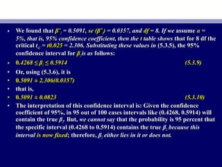
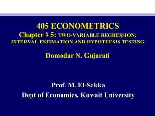
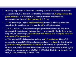
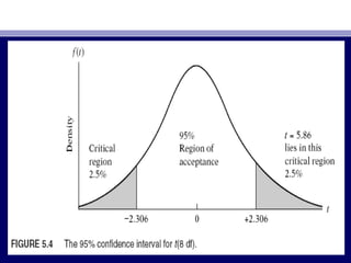
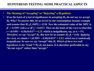
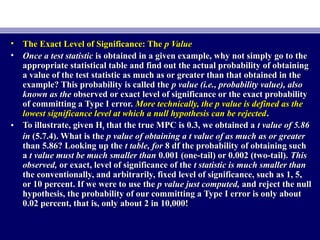
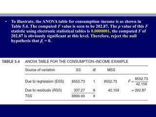
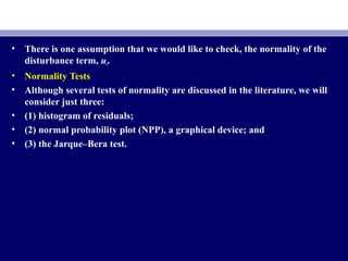
20. • The confidence-interval statementsThe confidence-interval statements such as the following can be made:such as the following can be made:
• Pr [−tPr [−tα/2α/2 ≤≤ ((βˆβˆ22 − β*− β*22)/se ()/se (βˆβˆ22) ≤) ≤ ttα/2α/2 ]=]= 1 − α1 − α (5.7.1)(5.7.1)
• wherewhere β*β*22 is the value ofis the value of ββ22 under Hunder H00.. Rearranging (5.7.1), we obtainRearranging (5.7.1), we obtain
• Pr [Pr [β*β*22 − t− tα/2α/2 se (se (βˆ2) ≤ βˆβˆ2) ≤ βˆ22 ≤ β*≤ β*22 + t+ tα/2α/2 se (se (βˆβˆ22)] = 1 − α)] = 1 − α (5.7.2)(5.7.2)
• which gives the confidence interval inwhich gives the confidence interval in with 1 − α probability.with 1 − α probability.
• (5.7.2) is known as(5.7.2) is known as the region of acceptancethe region of acceptance and theand the region(s) outside theregion(s) outside the
confidence interval is (are)confidence interval is (are) called the region(s) of rejection (ofcalled the region(s) of rejection (of HH00) or the) or the
critical regioncritical region(s).(s).
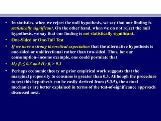
• Using consumption–income example. We know thatUsing consumption–income example. We know that βˆβˆ22 = 0.5091, se (βˆ= 0.5091, se (βˆ22) =) =
0.0357, and df = 8. If we assume α = 5 percent, t0.0357, and df = 8. If we assume α = 5 percent, tα/2α/2 = 2.306. If we let:= 2.306. If we let:
• HH00: β: β22 = β*= β*22 = 0= 0.3 and H1: β.3 and H1: β22 ≠≠ 0.3, (5.7.2) becomes0.3, (5.7.2) becomes
• Pr (0Pr (0.2177 ≤.2177 ≤ βˆβˆ22 ≤ 0.3823) = 0.95≤ 0.3823) = 0.95 (5.7.3)(5.7.3)
• Since the observedSince the observed βˆβˆ22 lies in thelies in the critical region, we reject the null hypothesiscritical region, we reject the null hypothesis
that truethat true ββ22 = 0.3.= 0.3.

22. • In practice, there is no need to estimate (5.7.2) explicitly.In practice, there is no need to estimate (5.7.2) explicitly. One can computeOne can compute
thethe t value in the middle of the double inequality given by (5.7.1)t value in the middle of the double inequality given by (5.7.1) andand seesee
whether it lies betweenwhether it lies between the critical t values or outside themthe critical t values or outside them. For our. For our example,example,
• t = (0.5091 − (0.3)) / (0.0357) = 5.86t = (0.5091 − (0.3)) / (0.0357) = 5.86 (5.7.4)(5.7.4)
• which clearly lies in the critical region of Figure 5.4. The conclusionwhich clearly lies in the critical region of Figure 5.4. The conclusion
remains the same; namely, we rejectremains the same; namely, we reject H0.H0.
• A statistic is said to be statistically significant if the value of the test statistic
lies in the critical region. By the same token, a test is said to be statistically
insignificant if the value of the test statistic lies in the acceptance region.
• We can summarize the t test of significance approach to hypothesis testing
as shown in Table 5.1.

25. • Testing the Significance ofTesting the Significance of σσ22
: The χ: The χ22
TestTest
• As another illustration of the test-of-significance methodology, consider theAs another illustration of the test-of-significance methodology, consider the
following variable:following variable:
• χχ22
== n − 2 (n − 2 (σσˆˆ22
// σσ22
)) (5.4.1)(5.4.1)
• which, as noted previously, follows thewhich, as noted previously, follows the χχ22
distribution with n − 2 df. For thedistribution with n − 2 df. For the
hypothetical example,hypothetical example, σσˆˆ22
= 42.1591 and df = 8. If we postulate that= 42.1591 and df = 8. If we postulate that
• HH00: σ: σ22
= 85 vs. H= 85 vs. H11: σ: σ22
≠≠ 85, Eq.85, Eq.
• (5.4.1) provides the test statistic for H(5.4.1) provides the test statistic for H00. Substituting. Substituting the appropriate values inthe appropriate values in
(5.4.1), it can be found that under(5.4.1), it can be found that under HH00, χ, χ22
= 3.97. If= 3.97. If we assumewe assume α = 5%, theα = 5%, the
critical χcritical χ22
values are 2.1797 and 17.5346.values are 2.1797 and 17.5346.
• Since theSince the computedcomputed χχ22
lies between these limits,lies between these limits, we do not rejectwe do not reject HH00. The. The χχ22
test of significance approach totest of significance approach to hypothesis testing is summarized in Tablehypothesis testing is summarized in Table
5.2.5.2.

27. HYPOTHESIS TESTING: SOME PRACTICALASPECTSHYPOTHESIS TESTING: SOME PRACTICALASPECTS
• The Meaning of “Accepting” or “Rejecting” a HypothesisThe Meaning of “Accepting” or “Rejecting” a Hypothesis
• If on the basis of a test of significance in accepting HIf on the basis of a test of significance in accepting H00, do not say we accept, do not say we accept
HH00. Why? To answer this, let us revert to our consumption–income example. Why? To answer this, let us revert to our consumption–income example
and assume thatand assume that HH00: β: β22 (MPC) = 0.50. Now(MPC) = 0.50. Now the estimated value of the MPC isthe estimated value of the MPC is
βˆβˆ22 = 0.5091 with a se (βˆ= 0.5091 with a se (βˆ22) = 0.0357. Then) = 0.0357. Then on the basis of theon the basis of the t test we find thatt test we find that
t = (0.5091 − 0.50)/0.0357 =t = (0.5091 − 0.50)/0.0357 = 0.25,0.25, which is insignificant, say, atwhich is insignificant, say, at α = 5%.α = 5%.
Therefore, we say “accept” HTherefore, we say “accept” H00. But. But now let us assumenow let us assume HH00: β: β22 = 0.48. Applying= 0.48. Applying
the t test, we obtain t = (0.5091 − 0.48)/0.0357 =the t test, we obtain t = (0.5091 − 0.48)/0.0357 = 0.820.82, which too is statistically, which too is statistically
insignificant. So now we sayinsignificant. So now we say “accept” this“accept” this HH00. Which of these two null. Which of these two null
hypotheses is the “truth”? We dohypotheses is the “truth”? We do not know. It is therefore preferable to saynot know. It is therefore preferable to say
“do not reject” rather than “accept.”“do not reject” rather than “accept.”

28. • The “Zero” Null Hypothesis and the “2-The “Zero” Null Hypothesis and the “2-t” Rule of Thumbt” Rule of Thumb
• A null hypothesis that is commonly tested in empirical work isA null hypothesis that is commonly tested in empirical work is HH00: β: β22 = 0,= 0,
that is, the slope coefficient is zero.that is, the slope coefficient is zero.
• This null hypothesis can be easily tested by the confidence interval or theThis null hypothesis can be easily tested by the confidence interval or the t-t-
test approach discussed in the preceding sections. But very often such formaltest approach discussed in the preceding sections. But very often such formal
testing can be shortcut by adopting the “2-testing can be shortcut by adopting the “2-t” rule of significance, whicht” rule of significance, which maymay
be stated asbe stated as

29. • The rationale for this rule is not too difficult to grasp. From (5.7.1) we knowThe rationale for this rule is not too difficult to grasp. From (5.7.1) we know
that we will rejectthat we will reject HH00: β: β22 = 0 if= 0 if
• t =t = βˆβˆ22 // se (se (βˆβˆ22) >) > ttα/2α/2 whenwhen βˆβˆ22 > 0> 0
oror
• t =t = βˆβˆ22 // se (se (βˆβˆ22) < −) < −ttα/2α/2 whenwhen βˆβˆ22 < 0< 0
or whenor when
• ||t| =t| = || βˆβˆ22 // se (se (βˆ2)βˆ2) || > t> tα/2α/2 (5.8.1)(5.8.1)
for the appropriate degrees of freedom.for the appropriate degrees of freedom.
• Now if we examine theNow if we examine the t, we see that for df oft, we see that for df of about 20 or more a computedabout 20 or more a computed tt
value in excess of 2 (in absolute terms), say,value in excess of 2 (in absolute terms), say, 2.1, is statistically significant at2.1, is statistically significant at
the 5 percent level, implying rejection of the null hypothesis.the 5 percent level, implying rejection of the null hypothesis.

30. • Forming the Null and Alternative HypothesesForming the Null and Alternative Hypotheses
• Very often the phenomenon under study will suggest the nature of the nullVery often the phenomenon under study will suggest the nature of the null
and alternative hypotheses. Consider the capital market line (CML) ofand alternative hypotheses. Consider the capital market line (CML) of
portfolio theory,portfolio theory,
• EEii = β= β11 + β+ β22σσii ,,
• where E = expected return onwhere E = expected return on portfolio andportfolio and σ = the standard deviation ofσ = the standard deviation of
return, a measure of risk. Sincereturn, a measure of risk. Since return and risk are expected to be positivelyreturn and risk are expected to be positively
related, natural alternative hypothesis to the null hypothesis thatrelated, natural alternative hypothesis to the null hypothesis that ββ22 = 0= 0
would be βwould be β22 > 0. That is, one would not choose to consider values> 0. That is, one would not choose to consider values ofof ββ22 lessless
than zero.than zero.
• Consider the case of the demand for money. Studies have shown that theConsider the case of the demand for money. Studies have shown that the
income elasticity of demand for money has typically ranged between 0.7income elasticity of demand for money has typically ranged between 0.7
and 1.3. Therefore, in a new study of demand for money, if one postulatesand 1.3. Therefore, in a new study of demand for money, if one postulates
that the income-elasticity coefficientthat the income-elasticity coefficient ββ22 is 1, the alternative hypothesis couldis 1, the alternative hypothesis could
be thatbe that ββ22 ≠≠ 1, a two-sided alternative hypothesis.1, a two-sided alternative hypothesis.
• Thus, theoretical expectations or prior empirical work or both can be reliedThus, theoretical expectations or prior empirical work or both can be relied
upon to formulate hypotheses.upon to formulate hypotheses.

31. • ChoosingChoosing α, the Level of Significanceα, the Level of Significance
• To reject or not reject the HTo reject or not reject the H00 depends critically ondepends critically on α,α, or theor the probability ofprobability of
committing acommitting a Type I error—theType I error—the probability of rejectingprobability of rejecting the true hypothesis.the true hypothesis.
But even then,But even then, why is α commonly fixed at the 1, 5, or at the most 10 percentwhy is α commonly fixed at the 1, 5, or at the most 10 percent
levelslevels? For a given sample size, if we try to reduce a? For a given sample size, if we try to reduce a Type I error, a Type IIType I error, a Type II
error increases, and viceerror increases, and vice versa. That is, given the sample size, if we try toversa. That is, given the sample size, if we try to
reduce the probability of rejecting the true hypothesis, we at the same timereduce the probability of rejecting the true hypothesis, we at the same time
increase the probability of accepting the false hypothesis.increase the probability of accepting the false hypothesis.
• Now the only way we can decide about the tradeoff is to find out the relativeNow the only way we can decide about the tradeoff is to find out the relative
costs of the two types of errors.costs of the two types of errors.
• Applied econometricians generally follow the practice of setting the value ofApplied econometricians generally follow the practice of setting the value of
α at a 1 or a 5 or at most a 10 percent level and choose a testα at a 1 or a 5 or at most a 10 percent level and choose a test statistic thatstatistic that
would make the probability of committing a Type II error as small aswould make the probability of committing a Type II error as small as
possible. Since one minus the probability of committing a Type II error ispossible. Since one minus the probability of committing a Type II error is
known as the power of the test, this procedure amounts to maximizing theknown as the power of the test, this procedure amounts to maximizing the
power of the test.power of the test.

32. • The Exact Level of Significance: TheThe Exact Level of Significance: The p Valuep Value
• Once a test statisticOnce a test statistic is obtained in a given example, why not simply go to theis obtained in a given example, why not simply go to the
appropriate statistical table and find out the actual probability of obtainingappropriate statistical table and find out the actual probability of obtaining
a value of the test statistic as much as or greater than that obtained in thea value of the test statistic as much as or greater than that obtained in the
example? This probability is called theexample? This probability is called the p value (i.e., probability value), alsop value (i.e., probability value), also
known as theknown as the observed or exact level of significance or the exact probabilityobserved or exact level of significance or the exact probability
of committing a Type I error.of committing a Type I error. More technically, the p value is defined as theMore technically, the p value is defined as the
lowest significance level at which a null hypothesis can be rejectedlowest significance level at which a null hypothesis can be rejected..
• To illustrate, given HTo illustrate, given H00 that the true MPC is 0.3, we obtained athat the true MPC is 0.3, we obtained a t value of 5.86t value of 5.86
inin (5.7.4). What is the(5.7.4). What is the p value of obtaining a t value of as much as or greaterp value of obtaining a t value of as much as or greater
than 5.86? Looking up thethan 5.86? Looking up the t table, fort table, for 8 df the probability of obtaining such8 df the probability of obtaining such
aa t value must be much smaller thant value must be much smaller than 0.001 (one-tail) or 0.002 (two-tail).0.001 (one-tail) or 0.002 (two-tail). ThisThis
observed,observed, or exact, level of significance of theor exact, level of significance of the t statistic is much smaller thant statistic is much smaller than
the conventionally, and arbitrarily, fixed level of significance, such as 1, 5,the conventionally, and arbitrarily, fixed level of significance, such as 1, 5,
or 10 percent. If we were to use theor 10 percent. If we were to use the p value just computed,p value just computed, and reject the nulland reject the null
hypothesis, the probability of our committing a Type I error is only abouthypothesis, the probability of our committing a Type I error is only about
0.02 percent, that is, only about 2 in 10,000!0.02 percent, that is, only about 2 in 10,000!

33. REGRESSION ANALYSIS AND ANALYSIS OF VARIANCEREGRESSION ANALYSIS AND ANALYSIS OF VARIANCE
• In Chapter 3, the following identity is developed:In Chapter 3, the following identity is developed:
• ΣΣyy22
ii =yˆ=yˆ22
ii ++ ΣΣuˆuˆ22
ii == βˆβˆ22
22 ΣΣxx22
ii ++ ΣΣuˆuˆ22
ii (3.5.2)(3.5.2)
• that is, TSS = ESS + RSS. A study of these components of TSS is known asthat is, TSS = ESS + RSS. A study of these components of TSS is known as
the analysis of variance (ANOVA).the analysis of variance (ANOVA).
• Associated with any sum of squares is its df, the number of independentAssociated with any sum of squares is its df, the number of independent
observations on which it is based. TSS hasobservations on which it is based. TSS has n − 1dfn − 1df because we lose 1 df inbecause we lose 1 df in
computing the sample meancomputing the sample mean Y¯. RSS hasY¯. RSS has n − 2dfn − 2df..
• ESS has 1 df which follows from the fact thatESS has 1 df which follows from the fact that
• ESS =ESS = βˆβˆ22
22 ΣΣxx22
ii is a function of βˆis a function of βˆ22
only, since xonly, since x22
ii is known.is known.
• Let us arrange the various sums of squares and their associated dfdf in Table
5.3, which is the standard form of the AOV table, sometimes called the
ANOVA table. Given the entries of Table 5.3, we now consider the following
variable:

34. • F = (MSS of ESS) / (MSS of RSS)
• = βˆ2
2 ΣΣ x2
i / (ΣΣ uˆ2
i / (n− 2)) (5.9.1)
• = βˆ2
2 ΣΣ x2
i / σˆ2
• If we assume that the disturbances ui are normally distributed, and if H0 is
that β2 = 0, then it can be shown that the F variable of (5.9.1) follows the F
distribution with 1 df in the numerator and (n − 2) df in the denominator.

35. • What use can be made of the preceding F ratio? It can be shown that
• Eβˆ2
2 ΣΣx2
i = σ2
+ β2
2 ΣΣx2
i (5.9.2)
• and
• E ΣΣuˆ2
i / n−2 = E(σˆ2
) = σ2
(5.9.3)
• (Note that β2 and σ2
appearing on the right sides of these equations are the
true parameters.) Therefore, if β2 is in fact zero, Eqs. (5.9.2) and (5.9.3) both
provide us with identical estimates of true σ2
. In this situation, the
explanatory variable X has no linear influence on Y whatsoever and the
entire variation in Y is explained by the random disturbances ui. If, on the
other hand, β2 is not zero, (5.9.2) and (5.9.3) will be different and part of the
variation in Y will be ascribable to X. Therefore, the F ratio of (5.9.1)
provides a test of the null hypothesis H0: β2 = 0.

36. • To illustrate, the ANOVA table for consumption–income is as shown in
Table 5.4. The computed F value is seen to be 202.87. The p value of this F
statistic using electronic statistical tables is 0.0000001, the computed F of
202.87 is obviously significant at this level. Therefore, reject the null
hypothesis that β2 = 0.

37. REPORTING THE RESULTS OF REGRESSION ANALYSIS
• Employing the consumption–income example of as an illustration:
• Yˆi = 24.4545 + 0.5091Xi
• se = (6.4138) (0.0357) r2 = 0.9621 (5.11.1)
• t = (3.8128) (14.2605) df = 8
• p = (0.002571) (0.000000289) F1,8 = 202.87
• Thus, for 8 df the probability of obtaining a t value of 3.8128 or greater is
0.0026 and the probability of obtaining a t value of 14.2605 or larger is
about 0.0000003.
• Under the null hypothesis that the true population intercept value is zero,
the p value of obtaining a t value of 3.8128 or greater is only about 0.0026.
Therefore, if we reject this null hypothesis, the probability of our
committing a Type I error is about 26 in 10,000. The true population
intercept is different from zero.

38. • If the true MPC were in fact zero, our chances of obtaining an MPC of
0.5091 would be practically zero. Hence we can reject the null hypothesis
that the true MPC is zero.
• Earlier we showed the intimate connection between the F and t statistics,
namely, F1, k = t2
k . Under the null hypothesis that the true β2 = 0, the F
value is 202.87, and the t value is about 14.24, as expected, the former value
is the square of the latter value.

39. EVALUATING THE RESULTS OF REGRESSION ANALYSIS
• How “good” is the fitted model? We need some criteria with which to
answer this question.
• First, are the signs of the estimated coefficients in accordance with
theoretical or prior expectations? e.g., the income consumption model
should be positive.
• Second, if theory says that the relationship should also be statistically
significant. The p value of the estimated t value is extremely small.
• Third, how well does the regression model explain variation in the
consumption expenditure? One can use r2
to answer this question, which is a
very high.

40. • There is one assumption that we would like to check, the normality of the
disturbance term, ui.
• Normality Tests
• Although several tests of normality are discussed in the literature, we will
consider just three:
• (1) histogram of residuals;
• (2) normal probability plot (NPP), a graphical device; and
• (3) the Jarque–Bera test.

41. • Histogram of Residuals.
• A histogram of residuals is a simple graphic device that is used to learn
something about the shape of the probability density function PDF of a
random variable.
• If you mentally superimpose the bell shaped normal distribution curve on
the histogram, you will get some idea as to whether normal (PDF)
approximation may be appropriate.

42. • Normal Probability Plot.
• A comparatively simple graphical device is the normal probability plot
(NPP). If the variable is in fact from the normal population, the NPP will be
approximately a straight line. The NPP is shown in Figure 5.7. We see that
residuals from our illustrative example are approximately normally
distributed, because a straight line seems to fit the data reasonably well.

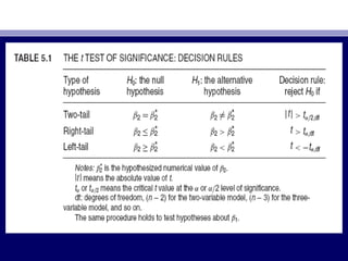
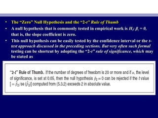
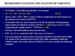
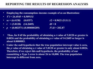
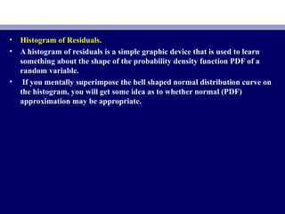
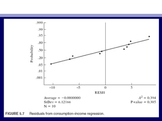
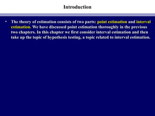
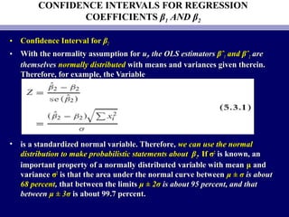
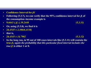
44. • Jarque–Bera (JB) Test of Normality.
• The JB test of normality is an asymptotic, or large-sample, test. It is also
based on the OLS residuals. This test first computes the skewness and
kurtosis, measures of the OLS residuals and uses the following test statistic:
• JB = n[S2
/ 6 + (K − 3)2
/ 24] (5.12.1)
• where n = sample size, S = skewness coefficient, and K = kurtosis coefficient.
For a normally distributed variable, S = 0 and K = 3. In that case the value
of the JB statistic is expected to be 0.

45. • The JB statistic follows the chi-square distribution with 2 df.
• If the computed p value of the JB statistic in an application is sufficiently
low, which will happen if the value of the statistic is very different from 0,
one can reject the hypothesis that the residuals are normally distributed. But if
the p value is reasonably high, which will happen if the value of the statistic
is close to zero, we do not reject the normality assumption.
• The sample size in our consumption–income example is rather small. If we
mechanically apply the JB formula to our example, the JB statistic turns
out to be 0.7769. The p value of obtaining such a value from the chi-square
distribution with 2 df is about 0.68, which is quite high. In other words, we
may not reject the normality assumption for our example. Of course, bear
in mind the warning about the sample size.

46. A CONCLUDING EXAMPLE
• Let us return to Example 3.2 about food expenditure in India. Using the
data given in (3.7.2) and adopting the format of (5.11.1), we obtain the
following expenditure equation:
• FoodExpˆi = 94.2087 + 0.4368 TotalExpi
• se = (50.8563) (0.0783)
• t = (1.8524) (5.5770)
• p = (0.0695) (0.0000)*
• r 2 = 0.3698; df = 53
• F1,53 = 31.1034 (p value = 0.0000)*

47. • As expected, there is a positive relationship between expenditure on food
and total expenditure. If total expenditure went up by a rupee, on average,
expenditure on food increased by about 44 paise.
• If total expenditure were zero, the average expenditure on food would be
about 94 rupees.
• The r2
value of about 0.37 means that 37 percent of the variation in food
expenditure is explained by total expenditure, a proxy for income.
• Suppose we want to test the null hypothesis that there is no relationship
between food expenditure and total expenditure, that is, the true slope
coefficient β2 = 0.

48. • The estimated value of β2 is 0.4368. If the null hypothesis were true, what is
the probability of obtaining a value of 0.4368? Under the null hypothesis,
we observe from (5.12.2) that the t value is 5.5770 and the p value of
obtaining such a t value is practically zero. In other words, we can reject the
null hypothesis. But suppose the null hypothesis were that β2 = 0.5. Now
what? Using the t test we obtain:
• t = 0.4368 − 0.5 / 0.0783 = −0.8071
• The probability of obtaining a |t | of 0.8071 is greater than 20 percent.
Hence we do not reject the hypothesis that the true β2is 0.5.

49. • Notice that, under the null hypothesis, the true slope coefficient is zero.
• The F value is 31.1034. Under the same null hypothesis, we obtained a t
value of 5.5770. If we square this value, we obtain 31.1029, which is about
the same as the F value, again showing the close relationship between the t
and the F statistic.
• Using the estimated residuals from the regression, what can we say about
the probability distribution of the error term? The information is given in
Figure 5.8. As the figure shows, the residuals from the food expenditure
regression seem to be symmetrically distributed.
• Application of the Jarque–Bera test shows that the JB statistic is about
0.2576, and the probability of obtaining such a statistic under the normality
assumption is about 88 percent. Therefore, we do not reject the hypothesis
that the error terms are normally distributed. But keep in mind that the
sample size of 55 observations may not be large enough.