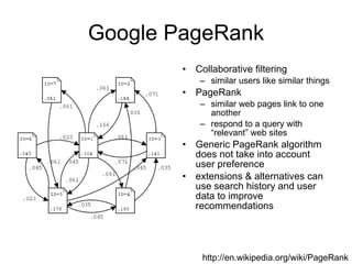
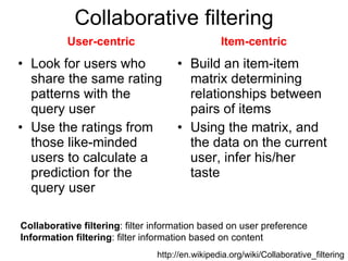
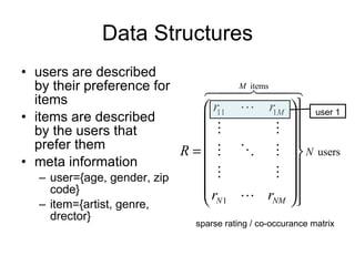
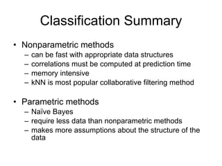
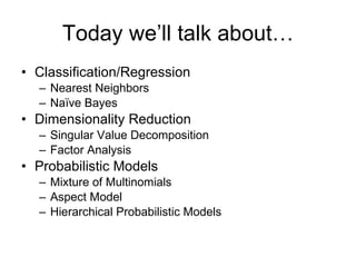
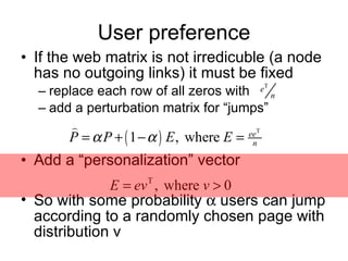
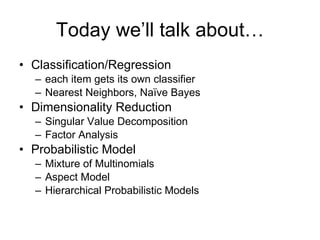
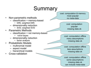
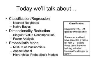
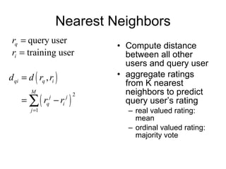
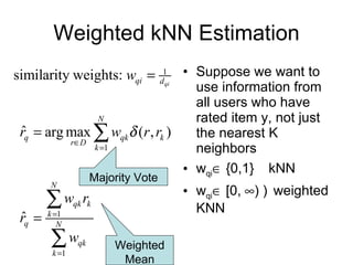
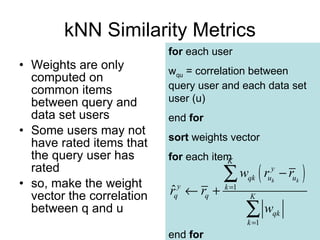
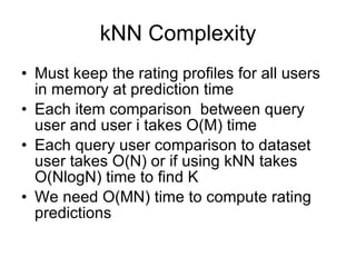
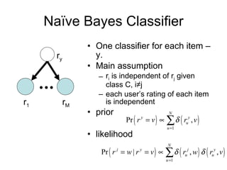
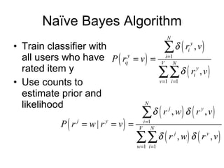
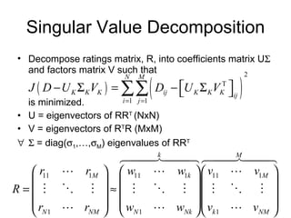
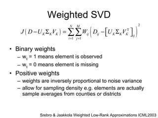
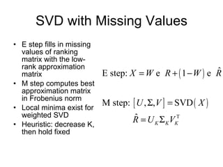
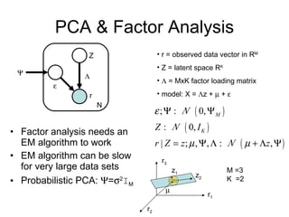
The document discusses several collaborative filtering techniques for making recommendations: 1) Nearest neighbor techniques like k-NN make predictions based on the ratings of similar users. They require storing all user data but can be fast with appropriate data structures. 2) Naive Bayes classifiers treat each item's ratings independently; they make strong assumptions but require less data. 3) Dimensionality reduction techniques like SVD decompose the user-item rating matrix to find latent factors. Weighted SVD handles missing data. 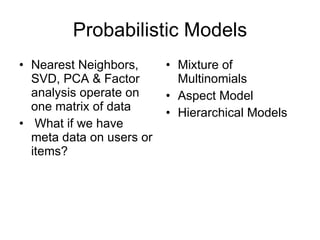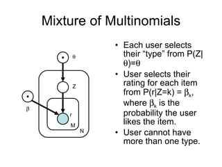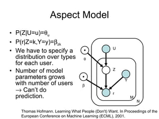4) Probabilistic models like mixtures of multinomials and aspect models represent additional user metadata but have more parameters.

1. Collaborative Filtering CS294 Practical Machine Learning Week 14 Pat Flaherty [email_address]

2. Amazon.com Book Recommendations If amazon.com doesn’t know me, then I get generic recommendations As I make purchases, click items, rate items and make lists my recommendations get “better”

3. Google PageRank Collaborative filtering similar users like similar things PageRank similar web pages link to one another respond to a query with “relevant” web sites Generic PageRank algorithm does not take into account user preference extensions & alternatives can use search history and user data to improve recommendations http://en.wikipedia.org/wiki/PageRank

4. Netflix Movie Recommendation http://www.netflixprize.com/ “ The Netflix Prize seeks to substantially improve the accuracy of predictions about how much someone is going to love a movie based on their movie preferences.”

5. Collaborative filtering Look for users who share the same rating patterns with the query user Use the ratings from those like-minded users to calculate a prediction for the query user Build an item-item matrix determining relationships between pairs of items Using the matrix, and the data on the current user, infer his/her taste http://en.wikipedia.org/wiki/Collaborative_filtering User-centric Item-centric Collaborative filtering : filter information based on user preference Information filtering : filter information based on content

6. Data Structures users are described by their preference for items items are described by the users that prefer them meta information user={age, gender, zip code} item={artist, genre, drector} sparse rating / co-occurance matrix user 1

7. Today we’ll talk about… Classification/Regression Nearest Neighbors Naïve Bayes Dimensionality Reduction Singular Value Decomposition Factor Analysis Probabilistic Model Mixture of Multinomials Aspect Model Hierarchical Probabilistic Models Classification Each item y=1,…,M gets its own classifier. Some users will not have recorded a rating for item y - discard those users from the training set when learning the classier for item y.

8. Nearest Neighbors Compute distance between all other users and query user aggregate ratings from K nearest neighbors to predict query user’s rating real valued rating: mean ordinal valued rating: majority vote

9. Weighted kNN Estimation Suppose we want to use information from all users who have rated item y, not just the nearest K neighbors w qi  {0,1}  kNN w qi  [0,  )  weighted KNN Majority Vote Weighted Mean

10. kNN Similarity Metrics Weights are only computed on common items between query and data set users Some users may not have rated items that the query user has rated so, make the weight vector the correlation between q and u for each user w qu = correlation between query user and each data set user (u) end for sort weights vector for each item end for

11. kNN Complexity Must keep the rating profiles for all users in memory at prediction time Each item comparison between query user and user i takes O(M) time Each query user comparison to dataset user takes O(N) or if using kNN takes O(NlogN) time to find K We need O(MN) time to compute rating predictions

12. Data set size examples MovieLens database 100k dataset = 1682 movies & 943 users 1mn dataset = 3900 movies & 6040 users Book crossings dataset after a 4 week long webcrawl 278,858 users & 271,378 books KDtrees & sparse matrix data structures can be used to improve efficiency

13. Naïve Bayes Classifier One classifier for each item – y. Main assumption r i is independent of r j given class C, i ≠j each user’s rating of each item is independent prior likelihood r 1 r M r y

14. Naïve Bayes Algorithm Train classifier with all users who have rated item y Use counts to estimate prior and likelihood

15. Classification Summary Nonparametric methods can be fast with appropriate data structures correlations must be computed at prediction time memory intensive kNN is most popular collaborative filtering method Parametric methods Naïve Bayes require less data than nonparametric methods makes more assumptions about the structure of the data

16. Today we’ll talk about… Classification/Regression Nearest Neighbors Naïve Bayes Dimensionality Reduction Singular Value Decomposition Factor Analysis Probabilistic Models Mixture of Multinomials Aspect Model Hierarchical Probabilistic Models

17. Singular Value Decomposition Decompose ratings matrix, R, into coefficients matrix U  and factors matrix V such that is minimized. U = eigenvectors of RR T (NxN) V = eigenvectors of R T R (MxM)  = diag(  1 ,…,  M ) eigenvalues of RR T

18. Weighted SVD Binary weights w ij = 1 means element is observed w ij = 0 means element is missing Positive weights weights are inversely proportional to noise variance allow for sampling density e.g. elements are actually sample averages from counties or districts Srebro & Jaakkola Weighted Low-Rank Approximations ICML2003

19. SVD with Missing Values E step fills in missing values of ranking matrix with the low-rank approximation matrix M step computes best approximation matrix in Frobenius norm Local minima exist for weighted SVD Heuristic: decrease K, then hold fixed

20. PageRank View the web as a directed graph Solve for the eigenvector with  =1 for the link matrix word id  web page list

21. PageRank Eigenvector Initialize r(P) to 1/n and iterate Or solve an eigenvector problem Link analysis, eigenvectors & stability http://ai.stanford.edu/~ang/papers/ijcai01-linkanalysis.pdf

22. Convergence If P is stochastic all rows sum to 1 non reducible (can’t get stuck), non periodic Then the dominant eigenvalue is 1 the left eigenvector is the stationary distribution of the Markov chain Intuitively, PageRank is the long-run proportion of time spent at that site by a web user randomly clicking links

23. User preference If the web matrix is not irredicuble (a node has no outgoing links) it must be fixed replace each row of all zeros with add a perturbation matrix for “jumps” Add a “personalization” vector So with some probability  users can jump according to a randomly chosen page with distribution v

24. PCA & Factor Analysis Factor analysis needs an EM algorithm to work EM algorithm can be slow for very large data sets Probabilistic PCA:  =  2 I M r = observed data vector in R M Z = latent space R K  = MxK factor loading matrix model: X =  z +  +  Z r     M =3 K =2 r 1 r 3 r 2 z 1 z 2 N

25. Matrix methods in general: recommendation does not depend on the particular item under consideration – only the similarity between query and dataset users one person may be a reliable recommender for another person with respect to a subset of items , but not necessarily for all possible items Thomas Hofmann. Learning What People (Don't) Want. In Proceedings of the European Conference on Machine Learning (ECML), 2001.

26. Dimensionality Reduction Summary Singular Value Decomposition requires one or more eigenvectors (one is fast, more is slow) Weighted SVD handles rating confidence measures handles missing data PageRank only need to solve a maximum eigenvector problem (iteration) “ user” preferences incorporated into Markov chain matrix for the web Factor Analysis extends Principle components analysis with a rating noise term

27. Today we’ll talk about… Classification/Regression each item gets its own classifier Nearest Neighbors, Naïve Bayes Dimensionality Reduction Singular Value Decomposition Factor Analysis Probabilistic Model Mixture of Multinomials Aspect Model Hierarchical Probabilistic Models

28. Probabilistic Models Nearest Neighbors, SVD, PCA & Factor analysis operate on one matrix of data What if we have meta data on users or items? Mixture of Multinomials Aspect Model Hierarchical Models

29. Mixture of Multinomials Each user selects their “type” from P(Z|  )=  User selects their rating for each item from P(r|Z=k) =  k , where  k is the probability the user likes the item. User cannot have more than one type. Z r  M N 

30. Aspect Model P(Z|U=u)=  u P(r|Z=k,Y=y)=  zk We have to specify a distribution over types for each user. Number of model parameters grows with number of users  Can’t do prediction. Z r  M N U Y  Thomas Hofmann. Learning What People (Don't) Want. In Proceedings of the European Conference on Machine Learning (ECML), 2001.

31. Hierarchical Models Meta data can be represented by additional random variables and connected to the model with prior & conditional probability distributions. Each user gets a distribution over groups,  u For each item, choose a group (Z=k), then choose a rating from that distribution Pr(r=v|Z=k)=  k Users can have more than one type (admixture). Z r  M N  

32. Cross Validation Before deploying a collaborative filtering algorithm we must make sure that it does well on new data Many machine learning methods fail at this stage real users change their behavior real data is not as nice as curated data sets

33. Support Vector Machine SVM is current state of the art classification algorithm We conclude that the quality of collaborative filtering recommendations is highly dependent on the quality of the data . Furthermore, we can see that kNN is dominant over SVM on the two standard datasets. On the real-life corporate dataset with high level of sparsity, kNN fails as it is unable to form reliable neighborhoods. In this case SVM outperforms kNN. http://db.cs.ualberta.ca/webkdd05/proc/paper25-mladenic.pdf

34. Data Quality If the accuracy of the algorithm depends on the quality of the data we need to look at how to select a good data set. Topic for next week… Active Learning, Sampling, Classical Experiment Design, Optimal Experiment Design, Sequential Experiment Design

35. Summary Non-parametric methods classification + memory-based kNN, weighted kNN dimensionality reduction SVD, weighted SVD Parametric Methods classification + not memory-based naïve bayes dimensionality reduction factor analysis Probabilistic Models multinomial model aspect model hierarchical models Cross-validation cost: computation & memory most popular no meta-data cost: computation popular missing data ok cost: computation offline many assumptions missing data ok cost: computation offline less assumptions missing data ok cost: computation offline some assumptions missing data ok can include meta-data

36. Boosting Methods Many simple methods can be combined to produce an accurate method with good generality

37. Clustering Methods Each user is an M-dimensional vector of item ratings Group users together Pros only need to modify N terms in distance matrix Cons regroup each time data set changes week 6 clustering lecture