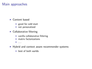
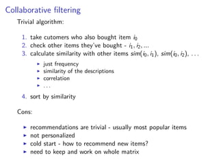
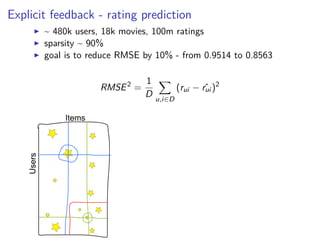
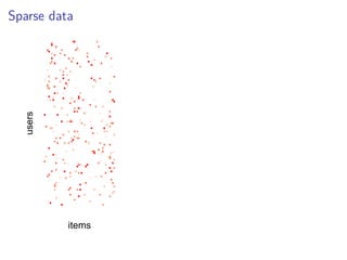
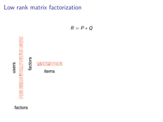
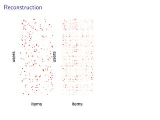
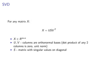
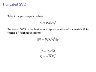
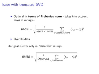
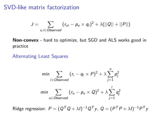
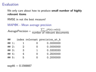
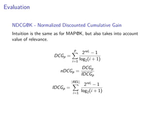
Matrix Factorizations for Recommender Systems
Dmitriy Selivanov
2017-08-26
Recommender systems are everywhere
Figure 1:
Recommender systems are everywhere
Figure 2:
Recommender systems are everywhere
Figure 3:
Recommender systems are everywhere
Figure 4:
Goals
Personalized offers
recommended items for a customer given history of activities
(transactions, browsing history, favourites)
Similar items
substitutions
frequently bought together
. . .
Exploration
Live demo
http://94.204.253.34/reco-playlist/
http://94.204.253.34/reco-similar-artists/
Main approaches
Content based
good for cold start
not personalized
Collaborative filtering
vanilla collaborative fitlering
matrix factorizations
. . .
Hybrid and context aware recommender systems
best of both worlds
Collaborative filtering
Trivial algorithm:
1. take cutomers who also bought item i0
2. check other items they’ve bought - i1, i2, ...
3. calculate similarity with other items sim(i0, i1), sim(i0, i2), . . .
just frequency
similarity of the descriptions
correlation
. . .
4. sort by similarity
Cons:
recommendations are trivial - usually most popular items
not personalized
cold start - how to recommend new items?
need to keep and work on whole matrix
User-based collaborative filtering
1. for a user u0 calculate sim(u0, U) and take top K
2. aggregate their opinions about items
weighted sum of their ratings
Cons:
cold start
nothing to recommend to new/untypical users
need to keep and work on whole matrix
Item-based collaborative filtering
1. for a item i0 calculate sim(i0, I) and take top K
2. show most similar items
Cons:
not personalized
cold start
Latent methods
Users can be described by small number of latent factors puk
Items can be described by small number of latent factors qki
Figure 5:
Netflix prize
Figure 6:
Explicit feedback - rating prediction
~ 480k users, 18k movies, 100m ratings
sparsity ~ 90%
goal is to reduce RMSE by 10% - from 0.9514 to 0.8563
RMSE2
=
1
D u,i∈D
(rui − ˆrui )2
Sparse data
items
users
Low rank matrix factorization
R = P ∗ Q
factors
users
items
factors
Reconstruction
items
users
items
users
SVD
For any matrix X:
X = USV T
X ∈ Rm∗n
U, V - columns are orthonormal bases (dot product of any 2
columns is zero, unit norm)
S - matrix with singular values on diagonal
Truncated SVD
Take k largest singular values:
X ≈ UkSkV T
k
Truncated SVD is the best rank k approximation of the matrix X in
terms of Frobenius norm:
||X − UkSkV T
k ||F
P = Uk
√
Sk
Q =
√
SkV T
k
Issue with truncated SVD
Optimal in terms of Frobenius norm - takes into account
zeros in ratings -
RMSE =
1
users × items u∈users,i∈items
(rui − ˆrui )2
Overfits data
Our goal is error only in “observed” ratings:
RMSE =
1
Observed u,i∈Observed
(rui − ˆrui )2
SVD-like matrix factorization
J =
u,i∈Observed
(rui − pu × qi )2
+ λ(||Q|| + ||P||)
Non-convex - hard to optimize, but SGD and ALS works good in
practice
Alternating Least Squares
min
i∈Observed
(ri − qi × P)2
+ λ
u
j=1
p2
j
min
u∈Observed
(ru − pu × Q)2
+ λ
i
j=1
q2
j
Ridge regression: P = (QT Q + λI)−1QT y, Q = (PT P + λI)−1PT y
Types of feedback
Explicit
Ratings, likes/dislikes, purchases
cleaner data
smaller
hard to collect
Implicit
Browsing, clicks, purchases, . . .
dirty data
larger datasets
generally gives better results
Implicit feedback
missed entries in matrix are mix of negative preferences and
positive preferences
consider them as negative with low confidence
observed entries are positive preferences
should have high confidence
Model - “Collaborative Filtering for Implicit Feedback Datasets”
Preferences
Pij =
1 if Rij > 0
0 otherwise
Confidence Cui = 1 + f (Rui )
Objective
J
u=user i=item
Cui (Pui − XuYi ) + λ(||X||F + ||Y ||F )
Alternating Least Squares for implicit feedback
For fixed Y :
dL/dxu = −2
i=item
cui (pui − xT
u yi )yi + 2λxu =
−2
i=item
cui (pui − yT
i xu)yi + 2λxu =
−2Y T
Cu
p(u) + 2Y T
Cu
Yxu + 2λxu
Setting dL/dxu = 0 for optimal solution gives us
(Y T CuY + λI)xu = Y T Cup(u)
xu can be obtained by solving system of linear equations:
xu = solve(Y T
Cu
Y + λI, Y T
Cu
p(u))
Alternating Least Squares for implicit feedback
Similarly for fixed X:
dL/dyi = −2XT Ci p(i) + 2XT Ci Yyi + 2λyi
yi = solve(XT Ci X + λI, XT Ci p(i))
Another optimization:
XT Ci X = XT X + XT (Ci − I)X
Y T CuY = Y T Y + Y T (Cu − I)Y
XT X and Y T Y can be precomputed
Evaluation
We only care about how to produce small number of highly
relevant items
RMSE in not the best measure!
MAP@K - Mean average precision
AveragePrecision =
n
k=1
(P(k)×rel(k))
number of relevant documents
## index relevant precision_at_k
## 1: 1 0 0.0000000
## 2: 2 0 0.0000000
## 3: 3 1 0.3333333
## 4: 4 0 0.2500000
## 5: 5 0 0.2000000
map@5 = 0.1566667
Evaluation
NDCG@K - Normalized Discounted Cumulative Gain
Intuition is the same as for MAP@K, but also takes into account
value of relevance.
DCGp =
p
i=1
2reli − 1
log2(i + 1)
nDCGp =
DCGp
IDCGp
IDCGp =
|REL|
i=1
2reli − 1
log2(i + 1)
Questions?
http://dsnotes.com/tags/recommender-systems/
http://94.204.253.34/reco-playlist/
http://94.204.253.34/reco-similar-artists/
Contacts:
selivanov.dmitriy@gmail.com
https://github.com/dselivanov

Recsys matrix-factorizations

  • 1.
    Matrix Factorizations forRecommender Systems Dmitriy Selivanov 2017-08-26
  • 2.
    Recommender systems areeverywhere Figure 1:
  • 3.
    Recommender systems areeverywhere Figure 2:
  • 4.
    Recommender systems areeverywhere Figure 3:
  • 5.
    Recommender systems areeverywhere Figure 4:
  • 6.
    Goals Personalized offers recommended itemsfor a customer given history of activities (transactions, browsing history, favourites) Similar items substitutions frequently bought together . . . Exploration
  • 7.
  • 8.
    Main approaches Content based goodfor cold start not personalized Collaborative filtering vanilla collaborative fitlering matrix factorizations . . . Hybrid and context aware recommender systems best of both worlds
  • 9.
    Collaborative filtering Trivial algorithm: 1.take cutomers who also bought item i0 2. check other items they’ve bought - i1, i2, ... 3. calculate similarity with other items sim(i0, i1), sim(i0, i2), . . . just frequency similarity of the descriptions correlation . . . 4. sort by similarity Cons: recommendations are trivial - usually most popular items not personalized cold start - how to recommend new items? need to keep and work on whole matrix
  • 10.
    User-based collaborative filtering 1.for a user u0 calculate sim(u0, U) and take top K 2. aggregate their opinions about items weighted sum of their ratings Cons: cold start nothing to recommend to new/untypical users need to keep and work on whole matrix
  • 11.
    Item-based collaborative filtering 1.for a item i0 calculate sim(i0, I) and take top K 2. show most similar items Cons: not personalized cold start
  • 12.
    Latent methods Users canbe described by small number of latent factors puk Items can be described by small number of latent factors qki Figure 5:
  • 13.
  • 14.
    Explicit feedback -rating prediction ~ 480k users, 18k movies, 100m ratings sparsity ~ 90% goal is to reduce RMSE by 10% - from 0.9514 to 0.8563 RMSE2 = 1 D u,i∈D (rui − ˆrui )2
  • 15.
  • 16.
    Low rank matrixfactorization R = P ∗ Q factors users items factors
  • 17.
  • 18.
    SVD For any matrixX: X = USV T X ∈ Rm∗n U, V - columns are orthonormal bases (dot product of any 2 columns is zero, unit norm) S - matrix with singular values on diagonal
  • 19.
    Truncated SVD Take klargest singular values: X ≈ UkSkV T k Truncated SVD is the best rank k approximation of the matrix X in terms of Frobenius norm: ||X − UkSkV T k ||F P = Uk √ Sk Q = √ SkV T k
  • 20.
    Issue with truncatedSVD Optimal in terms of Frobenius norm - takes into account zeros in ratings - RMSE = 1 users × items u∈users,i∈items (rui − ˆrui )2 Overfits data Our goal is error only in “observed” ratings: RMSE = 1 Observed u,i∈Observed (rui − ˆrui )2
  • 21.
    SVD-like matrix factorization J= u,i∈Observed (rui − pu × qi )2 + λ(||Q|| + ||P||) Non-convex - hard to optimize, but SGD and ALS works good in practice Alternating Least Squares min i∈Observed (ri − qi × P)2 + λ u j=1 p2 j min u∈Observed (ru − pu × Q)2 + λ i j=1 q2 j Ridge regression: P = (QT Q + λI)−1QT y, Q = (PT P + λI)−1PT y
  • 22.
    Types of feedback Explicit Ratings,likes/dislikes, purchases cleaner data smaller hard to collect Implicit Browsing, clicks, purchases, . . . dirty data larger datasets generally gives better results
  • 23.
    Implicit feedback missed entriesin matrix are mix of negative preferences and positive preferences consider them as negative with low confidence observed entries are positive preferences should have high confidence Model - “Collaborative Filtering for Implicit Feedback Datasets” Preferences Pij = 1 if Rij > 0 0 otherwise Confidence Cui = 1 + f (Rui ) Objective J u=user i=item Cui (Pui − XuYi ) + λ(||X||F + ||Y ||F )
  • 24.
    Alternating Least Squaresfor implicit feedback For fixed Y : dL/dxu = −2 i=item cui (pui − xT u yi )yi + 2λxu = −2 i=item cui (pui − yT i xu)yi + 2λxu = −2Y T Cu p(u) + 2Y T Cu Yxu + 2λxu Setting dL/dxu = 0 for optimal solution gives us (Y T CuY + λI)xu = Y T Cup(u) xu can be obtained by solving system of linear equations: xu = solve(Y T Cu Y + λI, Y T Cu p(u))
  • 25.
    Alternating Least Squaresfor implicit feedback Similarly for fixed X: dL/dyi = −2XT Ci p(i) + 2XT Ci Yyi + 2λyi yi = solve(XT Ci X + λI, XT Ci p(i)) Another optimization: XT Ci X = XT X + XT (Ci − I)X Y T CuY = Y T Y + Y T (Cu − I)Y XT X and Y T Y can be precomputed
  • 26.
    Evaluation We only careabout how to produce small number of highly relevant items RMSE in not the best measure! MAP@K - Mean average precision AveragePrecision = n k=1 (P(k)×rel(k)) number of relevant documents ## index relevant precision_at_k ## 1: 1 0 0.0000000 ## 2: 2 0 0.0000000 ## 3: 3 1 0.3333333 ## 4: 4 0 0.2500000 ## 5: 5 0 0.2000000 map@5 = 0.1566667
  • 27.
    Evaluation NDCG@K - NormalizedDiscounted Cumulative Gain Intuition is the same as for MAP@K, but also takes into account value of relevance. DCGp = p i=1 2reli − 1 log2(i + 1) nDCGp = DCGp IDCGp IDCGp = |REL| i=1 2reli − 1 log2(i + 1)
  • 28.