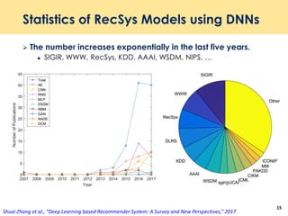
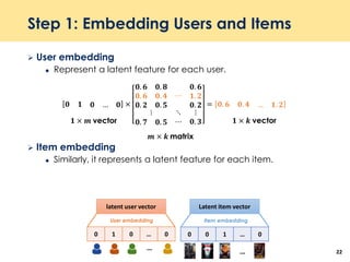
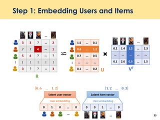
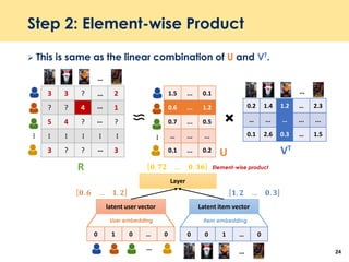
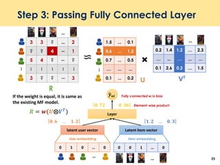
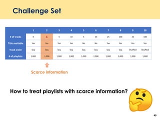
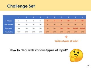
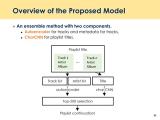
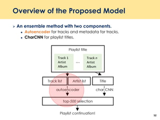
Downloaded 147 times


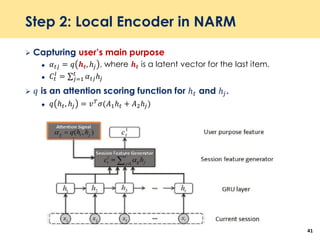
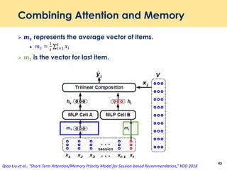
![Step 1: Global Encoder in NARM
Capturing user’s sequential behavior
ℎ 𝑡 = 1 − 𝑧𝑡 ℎ 𝑡−1 + 𝑧𝑡
ℎ 𝑡
𝑧𝑡 = 𝜎(𝑊𝑧 𝑥 𝑡 + 𝑈𝑧ℎ 𝑡−1) where 𝑧𝑡 is update gate
ℎ 𝑡 = tanh[𝑊𝑥 𝑡 + 𝑈 𝑟𝑡 ⊙ ℎ 𝑡−1 ]
𝑟𝑡 = 𝜎(𝑊𝑟 𝑥 𝑡 + 𝑈𝑟ℎ 𝑡−1)
40](https://image.slidesharecdn.com/recentadvancesindeeprecommendersystems-190925060403/85/Recent-advances-in-deep-recommender-systems-40-320.jpg)
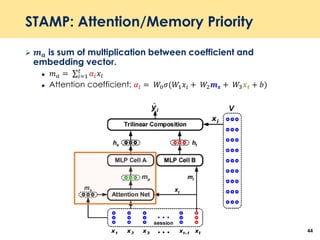
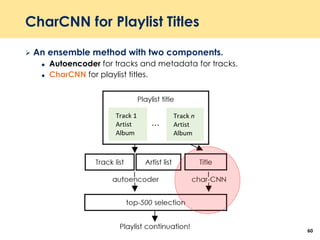
![Step 3: Decoder in NARM
Concatenated vector 𝑐𝑡 = 𝑐𝑡
𝑔
; 𝑐𝑡
𝑙
= [ℎ 𝑡
𝑔
; σ 𝑗−1
𝑡
𝛼 𝑡𝑗ℎ 𝑡
𝑙
]
Use an alternative bi-linear similarity function.
𝑆𝑖 = 𝑒𝑚𝑏𝑖
𝑇
𝐵𝑐𝑡 where 𝐵 is a 𝐷 × |𝐻| matrix.
|𝐷| is the dimension of each item.
42](https://image.slidesharecdn.com/recentadvancesindeeprecommendersystems-190925060403/85/Recent-advances-in-deep-recommender-systems-42-320.jpg)


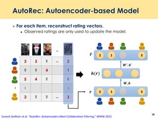
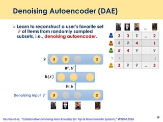
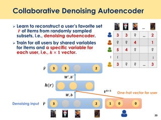
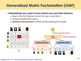
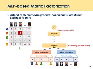
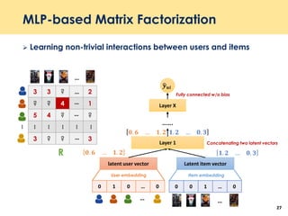
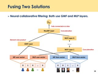
The document discusses recent advancements in deep learning-based recommender systems, highlighting the basics and methodologies such as collaborative filtering and matrix factorization. It explains various deep learning techniques used for product, movie, and music recommendations, along with challenges in modeling user-item interactions. Additionally, it explores specific models like AutoRec and Prod2Vec that utilize deep learning for improving recommendation accuracy.