Download as PDF, PPTX


![Prof. Pier Luca Lanzi
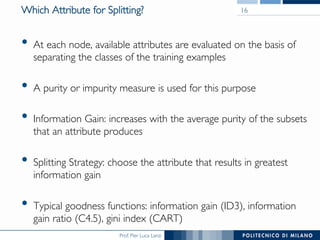
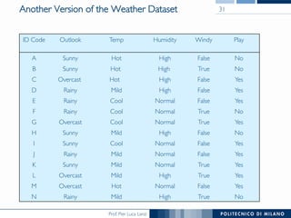
Information Gain Ratio for Weather Data 38
Outlook Temperature
Info: 0.693 Info: 0.911
Gain: 0.940-0.693 0.247 Gain: 0.940-0.911 0.029
Split info: info([5,4,5]) 1.577 Split info: info([4,6,4]) 1.362
Gain ratio: 0.247/1.577 0.156 Gain ratio: 0.029/1.362 0.021
Humidity Windy
Info: 0.788 Info: 0.892
Gain: 0.940-0.788 0.152 Gain: 0.940-0.892 0.048
Split info: info([7,7]) 1.000 Split info: info([8,6]) 0.985
Gain ratio: 0.152/1 0.152 Gain ratio: 0.048/0.985 0.049](https://image.slidesharecdn.com/dm2015-11-classificationtrees-150707165301-lva1-app6892/85/DMTM-2015-11-Decision-Trees-38-320.jpg)


![Prof. Pier Luca Lanzi
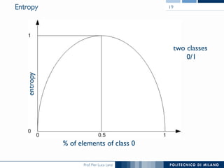
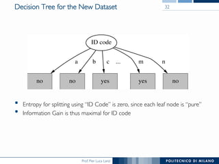
The Temperature Attribute
• First, sort the temperature values, including the class labels
• Then, check all the cut points and choose the one with the best
information gain
• E.g. temperature < 71.5: yes/4, no/2!
temperature ≥ 71.5: yes/5, no/3
• Info([4,2],[5,3]) = 6/14 info([4,2]) + 8/14 info([5,3]) = 0.939
• Place split points halfway between values
• Can evaluate all split points in one pass!
64 65 68 69 70 71 72 72 75 75 80 81 83 85
Yes No Yes Yes Yes No No Yes Yes Yes No Yes Yes No](https://image.slidesharecdn.com/dm2015-11-classificationtrees-150707165301-lva1-app6892/85/DMTM-2015-11-Decision-Trees-42-320.jpg)


![Prof. Pier Luca Lanzi
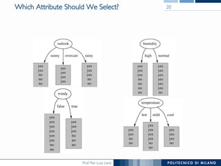
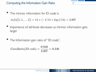
Mean and Variance
• Mean and variance for a Bernoulli trial: p, p (1–p)
• Expected error rate f=S/N has mean p and variance p(1–p)/N
• For large enough N, f follows a Normal distribution
• c% confidence interval [–z ≤ X ≤ z] for random variable with 0
mean is given by:
• With a symmetric distribution,
64](https://image.slidesharecdn.com/dm2015-11-classificationtrees-150707165301-lva1-app6892/85/DMTM-2015-11-Decision-Trees-64-320.jpg)
![Prof. Pier Luca Lanzi
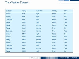
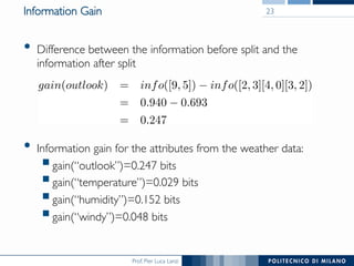
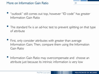
Confidence Limits
• Confidence limits for the
normal distribution with 0
mean and a variance of 1,
• Thus,
• To use this we have to
reduce our random
variable f to have 0 mean
and unit variance
65
Pr[X ≥ z] z
0.1% 3.09
0.5% 2.58
1% 2.33
5% 1.65
10% 1.28
20% 0.84
25% 0.69
40% 0.25](https://image.slidesharecdn.com/dm2015-11-classificationtrees-150707165301-lva1-app6892/85/DMTM-2015-11-Decision-Trees-65-320.jpg)


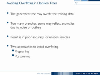
![Prof. Pier Luca Lanzi
Regression Trees for Prediction
• Decision trees can also be used to predict the value of a
numerical target variable
• Regression trees work similarly to decision trees, by analyzing
several splits attempted, choosing the one that minimizes impurity
• Differences from Decision Trees
! Prediction is computed as the average of numerical target
variable in the subspace (instead of the majority vote)
! Impurity is measured by sum of squared deviations from leaf
mean (instead of information-based measures)
! Find split that produces greatest separation in
[y – E(y)]2
! Find nodes with minimal within variance and therefore
! Performance is measured by RMSE (root mean squared error)
72](https://image.slidesharecdn.com/dm2015-11-classificationtrees-150707165301-lva1-app6892/85/DMTM-2015-11-Decision-Trees-72-320.jpg)


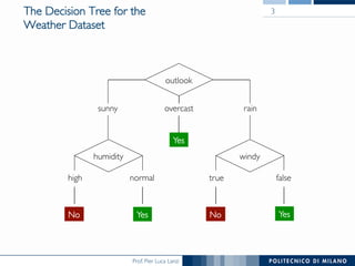
The document discusses decision trees and their construction. It begins by presenting the weather dataset with various attribute values and classifications. It then shows the decision tree constructed for this dataset, with internal nodes testing attributes and leaf nodes assigning a 'play' classification. The document goes on to explain the top-down induction of decision trees, considering attributes, stopping criteria, and how the best splitting attribute is determined using measures like information gain and information gain ratio to select the attribute that provides the most information about the target classification. It also addresses handling of numerical attributes through discretization.