Download as PDF, PPTX

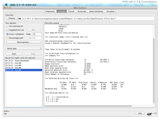
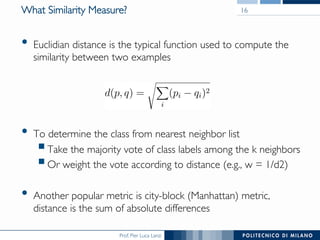
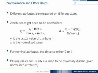
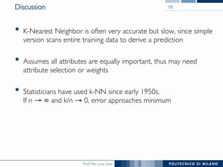
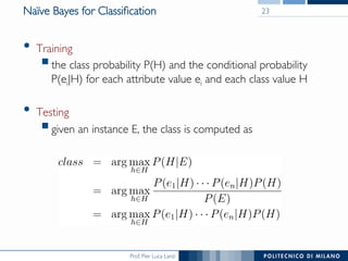
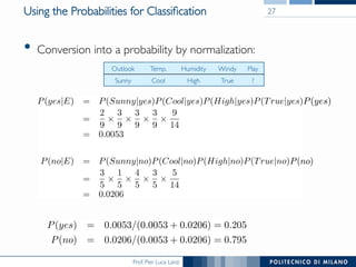
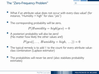
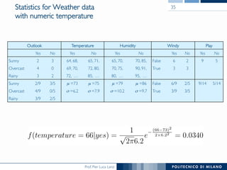
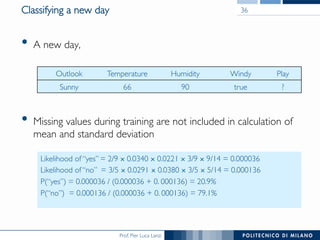
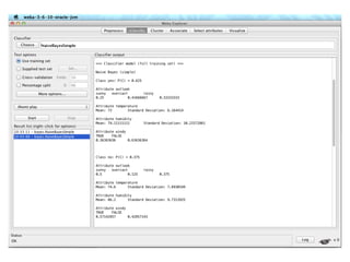
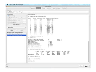
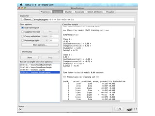
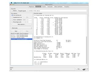
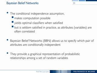

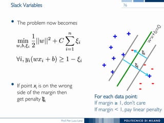
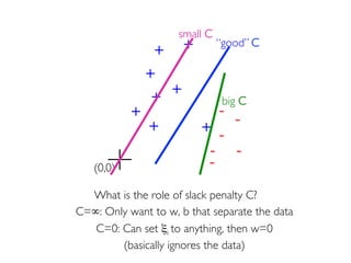
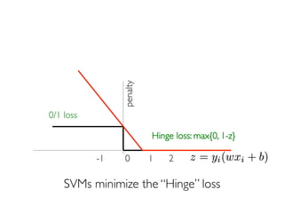
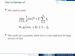


The document discusses various classification methods in data mining and instance-based learning, focusing on k-nearest neighbors and naïve Bayes classifiers. It explains how these methods operate, including distance metrics, training, testing, and their assumptions about data attributes. Additionally, it touches on logistic regression, Bayesian belief networks, and support vector machines, highlighting their mathematical foundations and practical applications.