Download as PDF, PPTX

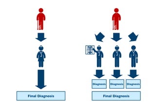
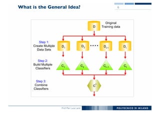
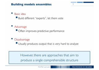

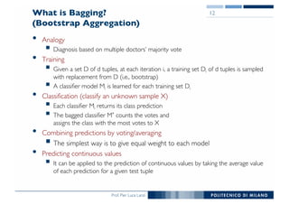
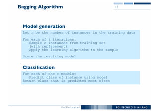
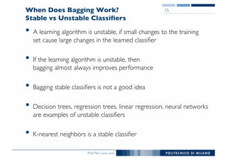


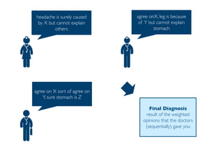
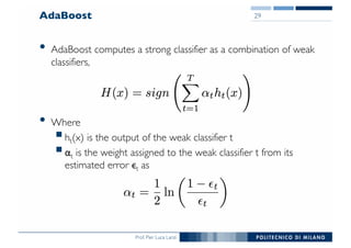
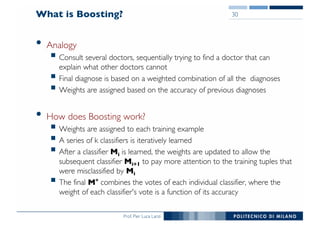
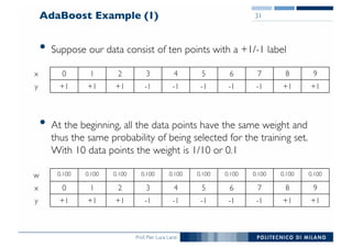
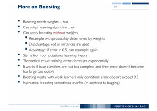
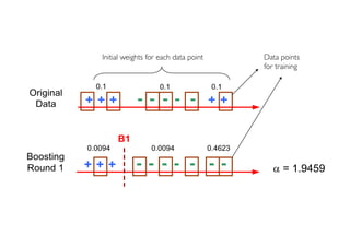
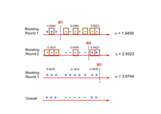
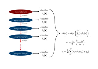
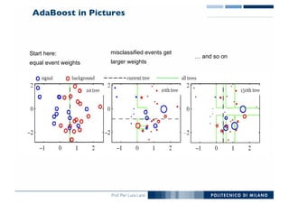


The document outlines ensemble methods in data mining, specifically focusing on bagging and boosting techniques like Random Forests and AdaBoost. Ensemble methods involve creating multiple classifiers from training data and aggregating their predictions to improve predictive performance, although they can complicate model analysis. Bagging stabilizes classifiers by reducing variance, while boosting sequentially enhances weak classifiers into a strong one by adjusting instance weights based on previous errors.


