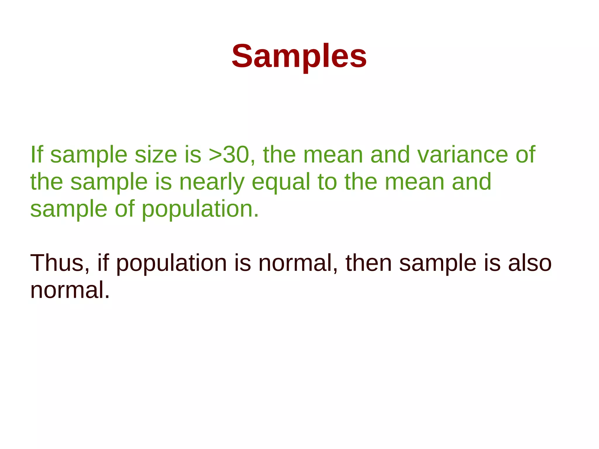
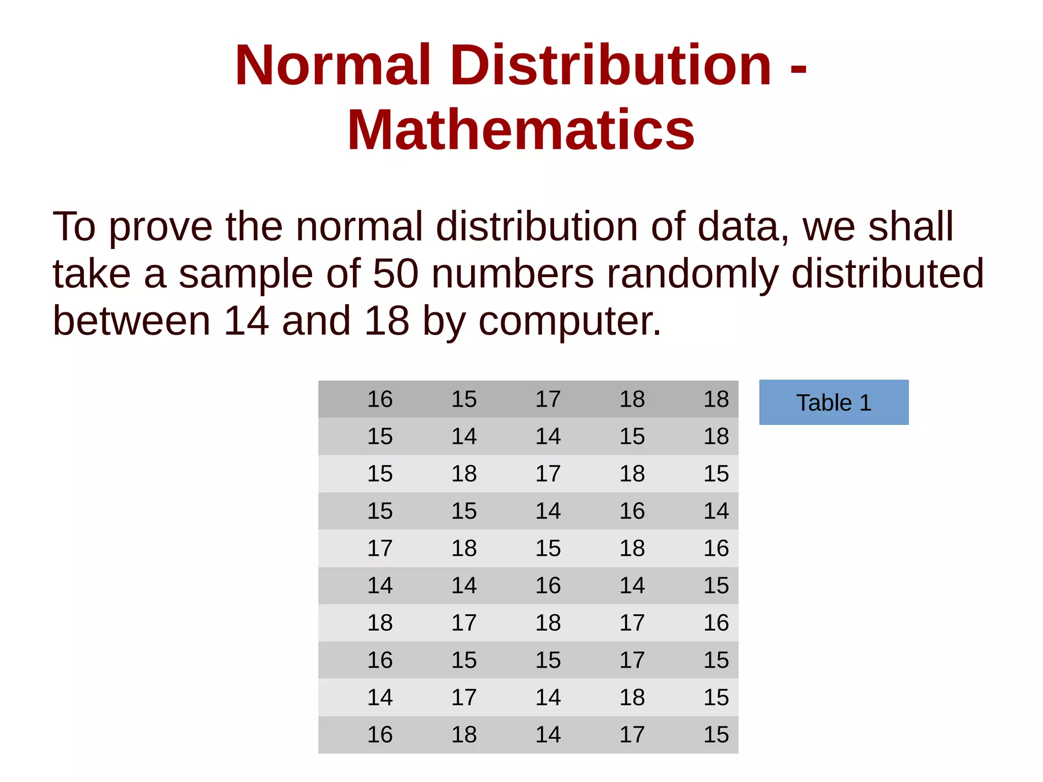
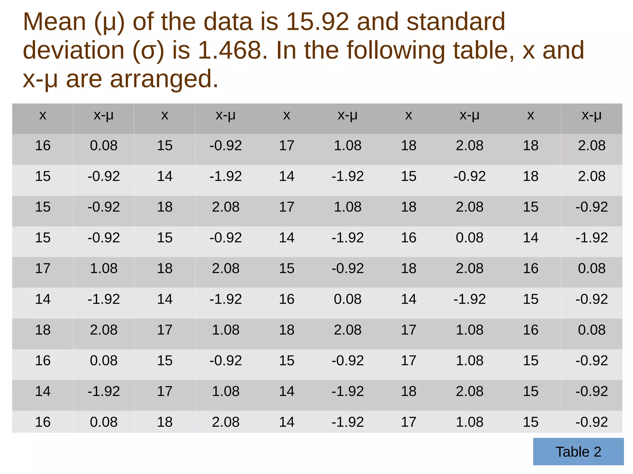
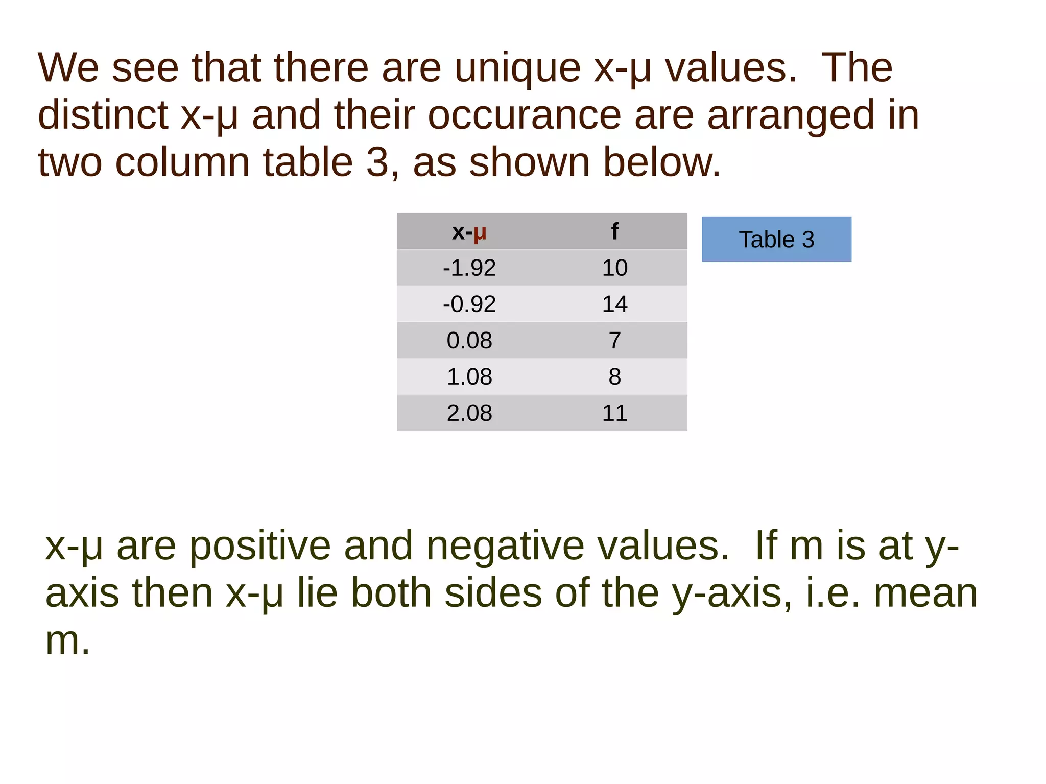
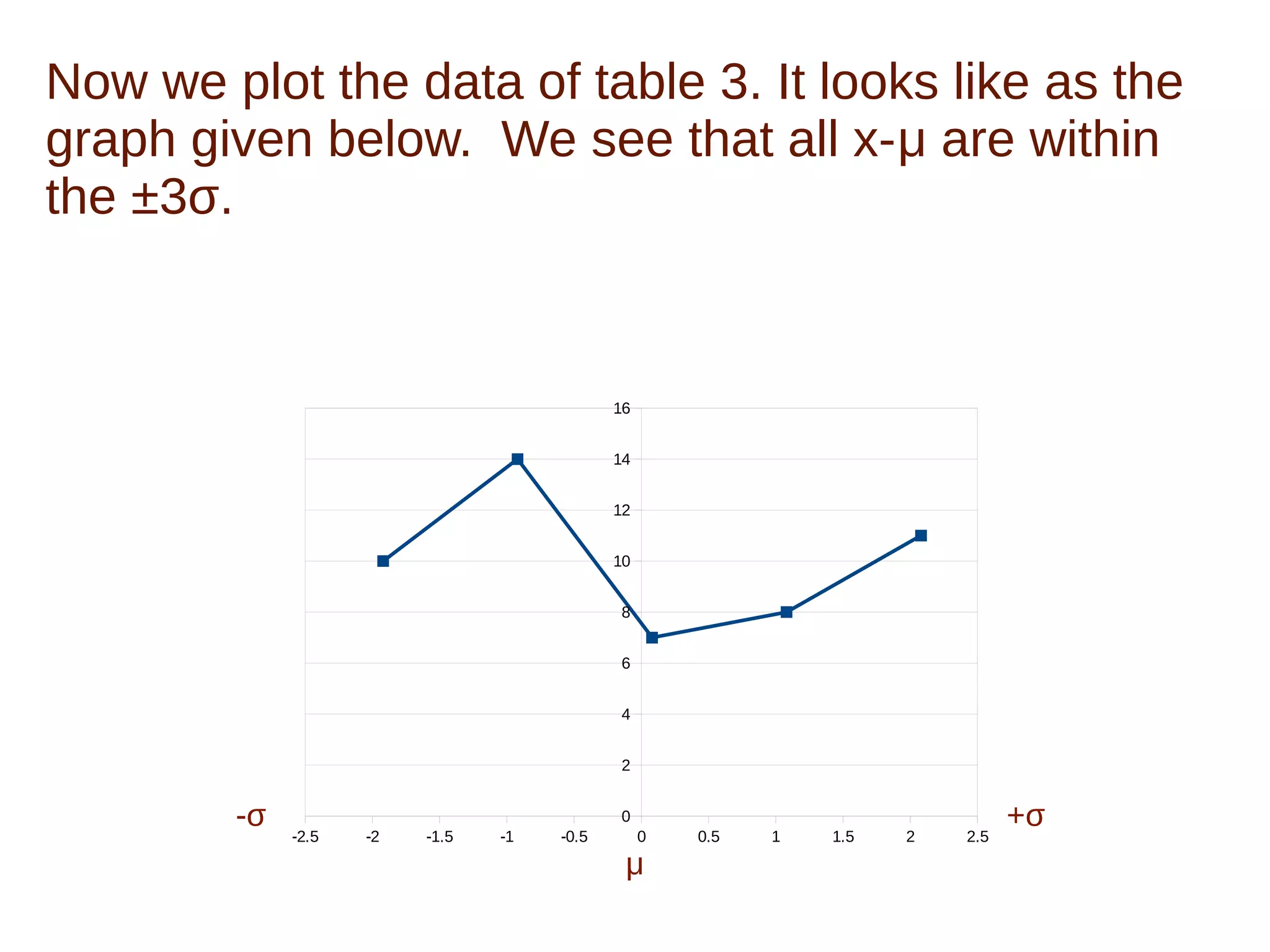
The document discusses the characteristics of normal data distribution, emphasizing its symmetry around the mean and the 99.7% of data within three standard deviations. It defines population and sample data, explaining the statistical properties that can be derived from each, particularly when sample sizes exceed 30. The text illustrates the normal distribution through mathematical examples and data plotting, concluding that real data typically produces an inverted bell shape in the distribution graph.

1. Distribution of Normal Data

2. Distribution of Normal Data
A data is said to be normal data if it is
symmetricaly distributed about its mean value and
99.7% of data is withing three times of standar
deviation about both side of mean.
The distibution curve of normal data about mean
is like inverted bell.

3. Population
Population is collection of all possible data.
Number of elements in population are very large.
Size of population is always kept large to
eliminate biasing for selection of particular
element.

4. Population
For example, if you have 10 billion random
numbers between 0 and 1, then probability of
biased selection of 0.0001001 is very small,
practically zero.
Mean or variance of population either given or
not. If mean and variance is not given, we can
not compute it mathematically due to large size of
data.

5. Samples
Sample is data that is collected from the
population.
Size of population is small, hence there is
probability of biased selection. We can compute
mean and variable of the sample.

6. Samples
If sample size is >30, the mean and variance of
the sample is nearly equal to the mean and
sample of population.
Thus, if population is normal, then sample is also
normal.

7. Normal Distribution -
Mathematics
To prove the normal distribution of data, we shall
take a sample of 50 numbers randomly distributed
between 14 and 18 by computer.
16 15 17 18 18
15 14 14 15 18
15 18 17 18 15
15 15 14 16 14
17 18 15 18 16
14 14 16 14 15
18 17 18 17 16
16 15 15 17 15
14 17 14 18 15
16 18 14 17 15
Table 1

8. x x-μ x x-μ x x-μ x x-μ x x-μ
16 0.08 15 -0.92 17 1.08 18 2.08 18 2.08
15 -0.92 14 -1.92 14 -1.92 15 -0.92 18 2.08
15 -0.92 18 2.08 17 1.08 18 2.08 15 -0.92
15 -0.92 15 -0.92 14 -1.92 16 0.08 14 -1.92
17 1.08 18 2.08 15 -0.92 18 2.08 16 0.08
14 -1.92 14 -1.92 16 0.08 14 -1.92 15 -0.92
18 2.08 17 1.08 18 2.08 17 1.08 16 0.08
16 0.08 15 -0.92 15 -0.92 17 1.08 15 -0.92
14 -1.92 17 1.08 14 -1.92 18 2.08 15 -0.92
16 0.08 18 2.08 14 -1.92 17 1.08 15 -0.92
Mean (μ) of the data is 15.92 and standard
deviation (σ) is 1.468. In the following table, x and
x-μ are arranged.
Table 2

9. x-μ f
-1.92 10
-0.92 14
0.08 7
1.08 8
2.08 11
We see that there are unique x-μ values. The
distinct x-μ and their occurance are arranged in
two column table 3, as shown below.
x-μ are positive and negative values. If m is at y-
axis then x-μ lie both sides of the y-axis, i.e. mean
m.
Table 3

10. -2.5 -2 -1.5 -1 -0.5 0 0.5 1 1.5 2 2.5
0
2
4
6
8
10
12
14
16
Now we plot the data of table 3. It looks like as the
graph given below. We see that all x-μ are within
the ±3σ.
+σ
μ
-σ

11. The graph is not like inverted bell shape. This is
due to less data grouping and small data size.
Here, data is generated by computer. This leads,
homogeniety of the data. Real data is unbiased,
independent and practical, which produce
inverted bell shape graph.
You can take other data and apply the same
method to find the normal data distribution curves.
Further check whether all data is distributed about
mean within ±3σ range or not.
This plot proves deviation of data about mean
within ±3σ visually.

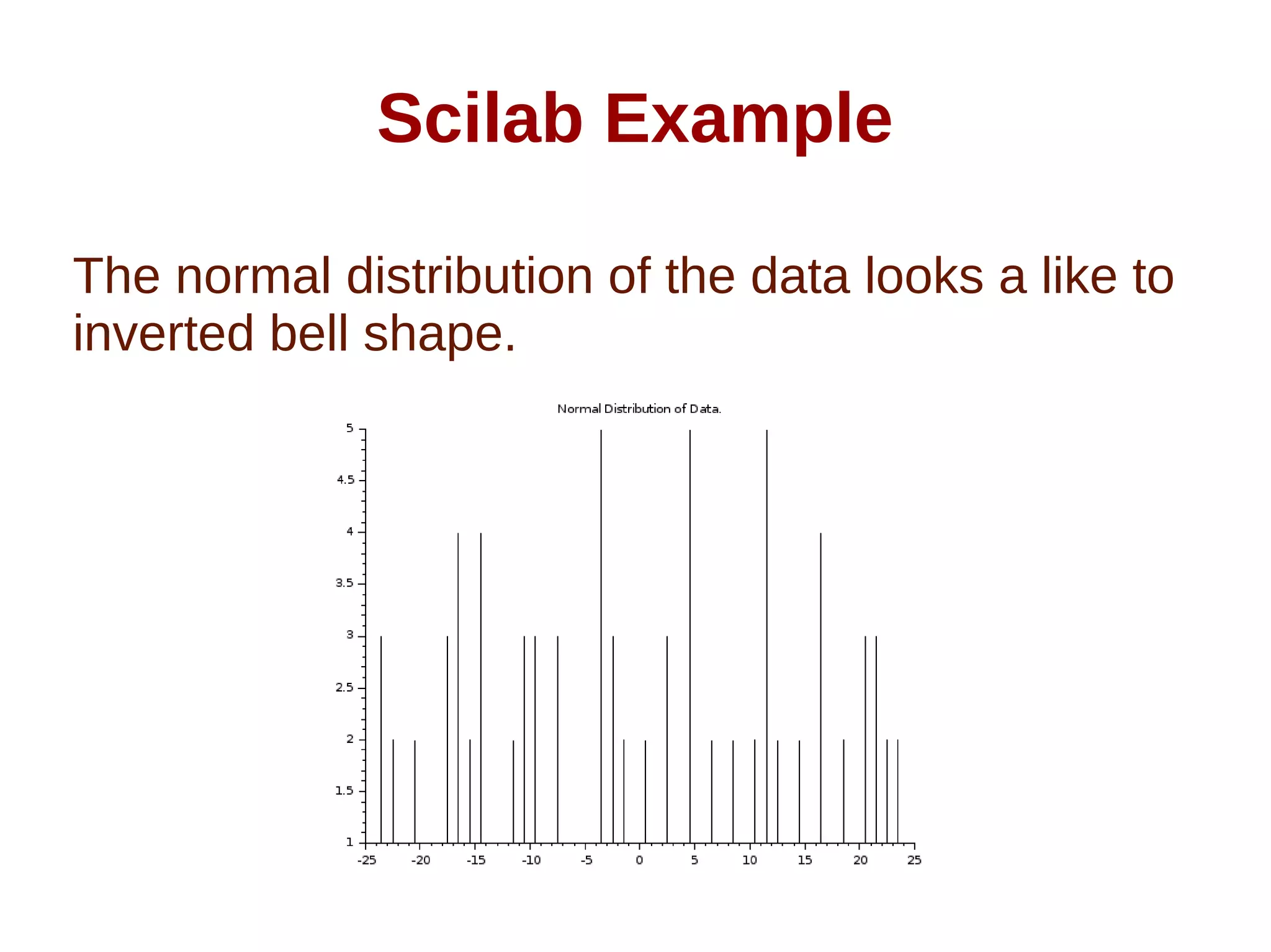
12. Scilab Example
● x=[442 401 412 416 437 406 428 447 439 408 411 403 448 415 438 410
440 414 446 434 408 443 419 426 447 425 429 442 441 428 436 449 423
431 434 409 424 402 445 430 402 407 418 450 422 409 448 428 414 437
437 411 411 446 430 415 422 447 410 415 404 430 426 433 446 422 437
444 440 430 418 436 420 421 432 409 423 444 424 423 449 405 422 411
442 422 432 417 402 403 409 430 416 408 437 405 416 438 418 442]
● m=mean(x);
● d=x-m
● f = tabul(d,"i");
● clf()
● plot2d3(f(:,1), f(:,2))
● xtitle("Normal Distribution of Data.")

13. Scilab Example
The normal distribution of the data looks a like to
inverted bell shape.