The document discusses key concepts related to the normal distribution, including its properties, formula, and uses. Some key points: - The normal distribution is a bell-shaped curve that is symmetric around the mean. Many natural phenomena approximate it. - It is defined by two parameters: the mean and standard deviation. Approximately 68% of values fall within one standard deviation of the mean, 95% within two standard deviations, and 99.7% within three standard deviations. - The normal distribution follows a specific formula involving the mean, standard deviation, and z-scores. 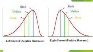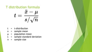- Other concepts discussed include skewness, kurtosis, the t-distribution and how it resembles the normal distribution, and

1. Theoretical distributions
and Unit root tests
Assoc Prof Ergin Akalpler

2. Normal Distribution: What It Is, Properties, Uses, and
Formula
 In graphical form, the normal distribution appears as a inverse
 "bell curve"
Normal distribution, also known as the Gaussian distribution, is a probability
distribution that is symmetric about the mean, showing that data near the mean
are more frequent in occurrence than data far from the mean.

3. KEY TAKEAWAYS
 The normal distribution is the proper term for a probability bell curve.
 In a normal distribution the mean is zero and the standard deviation is 1.
It has zero skew and a kurtosis of 3.
 Normal distributions are symmetrical, but not all symmetrical
distributions are normal.
 Many naturally-occurring phenomena tend to approximate the normal
distribution.
 In finance, most pricing distributions are not, however, perfectly normal.

4. Normal distribution
 The normal distribution is the most common type of
distribution assumed in technical stock market analysis
and in other types of statistical analyses. The standard
normal distribution has two parameters: the mean and the
standard deviation.

5. The normal distribution
 The normal distribution model is important in statistics and is
key to the Central Limit Theorem (CLT). This theory states that
averages calculated from independent, identically distributed
random variables have approximately normal distributions,
regardless of the type of distribution from which the variables
are sampled (provided it has finite variance).

6. Properties of the Normal Distribution
 The normal distribution has several key features and properties
that define it.
 First, its mean (average), median (midpoint), and mode (most
frequent observation) are all equal to one another.
 Moreover, these values all represent the peak, or highest point,
of the distribution.
 The distribution falls symmetrically around the mean, the width
of which is defined by the standard deviation.

7. The Empirical Rule
 For all normal distributions, 68.2% of the observations will
appear within plus or minus one standard deviation of the
mean;
 95.4% of the observations will fall within +/- two standard
deviations;
 and 99.7% within +/- three standard deviations. This fact is
sometimes referred to as the "empirical rule," a heuristic that
describes where most of the data in a normal distribution will
appear.

8. Empirical rule 68 – 95 – 99.7 For an approximately normal
data set,
the values within one
standard deviation of the
mean account for about
68% of the set;
while within two standard
deviations account for about
95%; and
within three standard
deviations account for about
99.7%.
St. de. Shown percentages
are rounded theoretical
probabilities intended only to
approximate the empirical
data derived from a normal
population.

10. Skewness
 Skewness measures the degree of symmetry of a distribution.
The normal distribution is symmetric and has a skewness of
zero.
 If the distribution of a data set instead has a skewness less
than zero, or negative skewness (left-skewness), then the left
tail of the distribution is longer than the right tail;
 positive skewness (right-skewness) implies that the right tail of
the distribution is longer than the left.

12. Kurtosis
 Kurtosis measures the thickness of the tail ends of a distribution in
relation to the tails of a distribution. The normal distribution has a
kurtosis equal to 3.0.
 Distributions with larger kurtosis greater than 3.0 exhibit tail data
exceeding the tails of the normal distribution (e.g., five or more
standard deviations from the mean). This excess kurtosis is known
in statistics as leptokurtic, "fat tails." The occurrence of fat tails in
financial markets describes what is known as tail risk.
 Distributions with low kurtosis less than 3.0 (platykurtic) exhibit
tails that are generally less extreme ("skinnier") than the tails of the
normal distribution.
 The Formula for

13. if the descriptive statistics estimated kurtosis value for all considered parameters are positive,
which implies that the distribution has heavier tails and a sharper peak than normal distribution.
Furthermore, in a distribution where a negative kurtosis value is observed, the curve has lighter
tails and a flatter peak or more rounded curve than the normal distribution, which is not
observed in this study. In Figure 2 below, the solid line indicates the normal distribution and
the dotted line shows the positive kurtosis values.
Figure 2: Positive Kurtosis

14. The Formula for the Normal Distribution
 The normal distribution follows the following formula. Note that
only the values of the mean (μ ) and standard deviation (σ) are
necessary
 Normal Distribution Formula
Z score and standard deviation relation
Z-score indicates how much a given value differs from the standard
deviation.
The Z-score, or standard score, is the number of standard deviations
a given data point lies above or below mean. Standard deviation is
essentially a reflection of the amount of variability within a given data set.

15. Sample question
 Let us consider and use the normal distribution table and find the area
 Use the standard formula Z= X-µ/σ
 Z Score = ( X – µ ) / σ
 Where
 Z ; average percentage value
 X is a normal random variable
 µ average mean value
 σ standard deviation
 example µ= 5 and σ= 2 in a normal distribution please find the deviation area between x=6 and
x=9
 First you have to find these standard deviation
 Z= 6-5/2=0.5
 Z=9-5/2= 2 and then we will look standard normal distribution table for 0.5 it is 0.6915
 and for 2 it is 0.9772 and when we subtract each other 0.9772-6915= 0.2857 this gives us the
area between 6 and 9 which is 28.57%

16. Example 2
 lets find µ=5 and σ=2 for the standard deviation area when x=1 and x=3
 Z= 1-5/2=-2
 And z 3-5/2=-1
 if it is negative for -1 subtract from 0.5 to find left side value of normal
distribution table 0.8413-0.5000= -0.3413
 for the -2 from table
 0.9772-0.5000=0.4772
 Z=1 is 0.3413 and z=2 is 0.4772
 Subtract from each other 0.4772-0.3413=0.1359

17. Normal Distribution table

18. Example
 Assuming the weight of an orange is 200 g and the mean standard deviation is
determined as 50 g, what will be the percentage of oranges 300 g and above,
assuming that the oranges have a normal distribution?
 Z= X-µ/σ 300-200/50=2 or (X=300) The area to the right is found by subtracting
0.4772 from half of the symmetric normal distribution (the area is 0.4772 if we
subtract this from 0.5000)
 This value is 0.5-0.4772=0.0228, so 2.28 percent of oranges are heavier than
300 grams.


19. How to develop a hypothesis
 Another question regarding the distribution of the weights of the oranges
mentioned above is what value is the weight of 60 percent of the
oranges below. As shown in the figure, we need to find the z value in
order to find the x value hypothesis generation
 Ho whole oranges 300+
 H1: whole oranges 200+50If the
 HO is in the acceptance zone arithmetically, it is rejected if not
accepted. And here H1 is accepted because the arithmetic mean is in
the reject region.

20. T distribution
 The t distribution is a symmetrical distribution and its appearance
resembles a normal distribution.
 If the data is less than 30, the t distribution table is used.
 If the sample volume commands, the standard normal distribution
table is used instead of the t distribution, because the larger the
sample volume, the closer the t distribution to the standard normal
distribution.

21. T distribution formula
t = t-distribution
x = sample mean
µ = population mean
s = sample standard deviation
n = sample size

22. Example
For example, let n = 15, let's find the value of t, which represents a 40% area
at t=0.
In the distribution table, when we subtract the value of 0.4, which means 40%,
from the value of 0.5,
0.5-0.4=0.10 which is half of the total area,
for the area of 40% in question, we will obtain the value of t, which is given
according to the value of 0.1, and the standard deviation.
We find at the intersection of =n-1= 15-1=14 line, this t value is 1.345 and it
is shown as td (14)= 1.345.
t = t-distribution
x = sample mean
µ = population mean
s = sample standard deviation
n = sample size