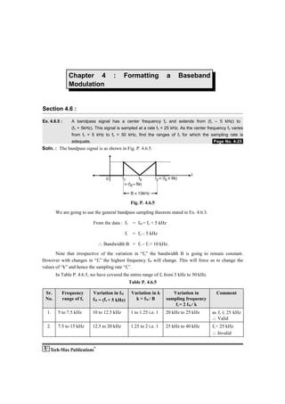
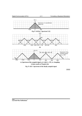
SlideShare a Scribd company logo
Digital Communication (GTU)                            4-1                 Formatting a Baseband Modulation


              Chapter 4              :      Formatting                 a    Baseband
              Modulation


Section 4.6 :

Ex. 4.6.5 :    A bandpass signal has a center frequency fo and extends from (fo – 5 kHz) to
               (fo + 5kHz). This signal is sampled at a rate f s = 25 kHz. As the center frequency fo varies
               from fo = 5 kHz to fo = 50 kHz, find the ranges of fo for which the sampling rate is
               adequate.                                                                    .Page No. 4-25.
Soln. : The bandpass signal is as shown in Fig. P. 4.6.5.


                                                 Fig. P. 4.6.5

       We are going to use the general bandpass sampling theorem stated in Ex. 4.6.3.

                           From the data : f2      = fM = fo + 5 kHz

                                            f1     = fo – 5 kHz

                             ∴ Bandwidth B = f2 – f1 = 10 kHz.

       Note that irrespective of the variation in “fo” the bandwidth B is going to remain constant.
However with changes in “fo” the highest frequency fM will change. This will force us to change the
values of “k” and hence the sampling rate “fs”.
       In Table P. 4.6.5, we have covered the entire range of fo from 5 kHz to 50 kHz.
                                                 Table P. 4.6.5

 Sr.      Frequency        Variation in fM        Variation in k        Variation in          Comment
 No.      range of fo      fM = (fo + 5 kHz)        k = fM / B       sampling frequency
                                                                         fs = 2 fM / k
  1.    5 to 7.5 kHz       10 to 12.5 kHz         1 to 1.25 i.e. 1   20 kHz to 25 kHz       as fs ≤ 25 kHz
                                                                                            ∴ Valid
  2.    7.5 to 15 kHz      12.5 to 20 kHz         1.25 to 2 i.e. 1   25 kHz to 40 kHz       fs > 25 kHz
                                                                                            ∴ Invalid
Digital Communication (GTU)                            4-2                Formatting a Baseband Modulation

 Sr.         Frequency       Variation in fM      Variation in k        Variation in          Comment
 No.         range of fo     fM = (fo + 5 kHz)      k = fM / B       sampling frequency
                                                                         fs = 2 fM / k
     3.    15 to 20 kHz      20 to 25 kHz         2 to 2.5 i.e. 2    20 kHz to 25 kHz       fs ≤ 25 kHz
                                                                                            ∴ Valid
     4.    20 to 25 kHz      25 to 30 kHz         2.5 to 3 i.e. 2    25 kHz to 30 kHz       fs > 25 kHz
                                                                                            ∴ Invalid
     5.    25 to 32.5 kHz    30 to 37.5 kHz       3 to 3.75 i.e. 3   20 kHz to 25 kHz       fs ≤ 25 kHz
                                                                                            ∴ Valid
     6.    32.5 to 35 kHz    37.5 to 40 kHz       3.75 to 4 i.e. 3   25 kHz to 26.66 kHz    fs > 25 kHz
                                                                                            ∴ Invalid
     7.    35 to 45 kHz      40 to 50 kHz         4 to 5 i.e. 4      20 kHz to 25 kHz       fs < 25 kHz
                                                                                             ∴ Valid
     8.    45 to 50 kHz      50 to 55 kHz         5 to 5.5 i.e. 5    20 kHz to 22 kHz       fs < 25 kHz
                                                                                            ∴ Valid

Conclusion :
       From Table P. 4.6.5 it is evident that the sampling rate of 25 kHz is adequate for the following
frequency ranges of “fo” :
1.        5 to 7.5 kHz       2.   15 to 20 kHz
3.        25 to 32.5 kHz     4.   35 to 50 kHz.

Ex. 4.6.6 :       The signals x1 (t) = 10 cos (100 πt) and x2 (t) = 10 cos (50 πt) are both sampled at times
                  tn = n / fs where n = 0, ± 1, ± 2, ... and the sampling frequency is 75 samples/sec. Show
                  that the two sequences of samples thus obtained are identical. What is this phenomenon
                  called ?                                                                  .Page No. 4-25.
Soln. :
          Let us prove that we get the identical sequences of samples by using the graphical method.
      The signals x1 (t) and x2 (t) are cosine waves with equal peak amplitudes. Their frequencies are 50
Hz and 25 Hz respectively.

                  ∴ x1 ( t ) : Has peak voltage = 10 V and f1 = 50 Hz

                  ∴ x2 ( t ) : Has peak voltage = 10 V and f2 = 25 Hz

      The sampling frequency fs = 75 Hz and sampling period Ts = 1/75 = 13.33 ms. Steps to be
followed to plot the sampled versions are as follows :
Step 1 : Draw the signals x1 ( t ), x2 ( t ) and the sampling function.
Step 2 : Encircle the sample values.
Step 3 : Draw the sampled signals x1 δ ( t ) and x2 δ ( t ).
Digital Communication (GTU)                        4-3                Formatting a Baseband Modulation

       All these waveforms are as shown in Fig. P. 4.6.6.


                                              Fig. P. 4.6.6
Conclusion :
        The sampling frequency of 75 Hz is lower than the Nyquist rate. Because to sample a 50 Hz
signal the sampling rate should atleast be 100 Hz. Therefore aliasing takes place. The identical sequence
in Fig. P. 4.6.6 are being obtained due to aliasing.

Section 4.7 :

Ex. 4.7.3 :    A signal x (t) = cos 200 πt + 2 cos 320 πt is ideally sampled at fs = 300 Hz. If the sampled
               signal is passed through an ideal low pass filter with a cutoff frequency of 250 Hz, what
               frequency components will appear in the output?                            .Page No. 4-27.

Soln. : It has been given that x (t) = cos 200 πt + 2 cos 320 πt and fS = 300 Hz. The spectrum of the
ideally sampled signal is given by,

                                   Xδ (f) = fs X (f – n fs) = 300 X (f – 300 n)

                                          = 300 X (f) + 300 X (f ± 300) + 300 X (f ± 600) + …        ...(1)

•   The spectrum of x (t) is as shown in Fig. P. 4.7.3(a) which contains two frequency components
    f1 = 100 Hz and f2 = 160 Hz.
•   The second term in Equation (1) shows X (f) centered about ± fs = 300 Hz.
Digital Communication (GTU)                         4-4                 Formatting a Baseband Modulation


•   The spectrum shifted towards right (see Fig. P. 4.7.3(b)) consists of four frequency components as
    follows :
                                   fs + f1 = 300 + 100 = 400 Hz


                                               Fig. P. 4.7.3

Ex. 4.7.4 :   Fig. P. 4.7.4(a) shows the spectrum of a low-pass signal g (t). The signal is sampled at
              the rate of 1.5 Hz and then applied to a low-pass reconstruction filter with cut-off
              frequency at 1 Hz.
              1.    Plot the spectrum of the sampled signal and specify distortion, if any.
              2.    If the low-pass reconstruction filter is to faithfully reproduce g (t) at its output, what
                    should be the minimum sampling frequency ?                               .Page No. 4-27.
Digital Communication (GTU)                          4-5                Formatting a Baseband Modulation


                                              Fig. P. 4.7.4(a)

Soln. : Given : Sampling frequency fs = 1.5 Hz
                Cut-off frequency of a low pass filter fcut – off = 1 Hz.

1.     Spectrum of the sampled signal :
       The spectrum of sampled signal is given by,
                                       Gδ (f) = fs G (f – nfs)
       The spectrum of the sampled signal is as shown in Fig. P. 4.7.4(b).
       As shown in Fig. P. 4.7.4(b) the spectrums overlap giving rise to a distortion called “Aliasing”.
2.     If a low pass filter is to faithfully reproduce g (t) then the minimum sampling rate should be
                                    fs (min) = 2 × 1 = 2 Hz                                        ...Ans.


                           Fig. P. 4.7.4(b) : Spectrum of the sampled signal

Ex. 4.7.5 :    A signal g(t) contains two frequencies 1000 Hz and 5000 Hz expressed as
               g (t) = (cos 6280 t + cos 31400 t). It is sampled at 8000 samples/sec. Determine the
               spectrum of sampled signal and plot the spectrum. Assume instantaneous sampling. This
               sampled signal is passed through a LPF with constant unity gain from 0 to 2 kHz and
Digital Communication (GTU)                            4-6            Formatting a Baseband Modulation


               linearly decreasing gain from 2 kHz to 4 kHz with a zero gain at 4 kHz. Determine the
               output and interpret the result.                                        .Page No. 4-27.
Soln. :
Step 1 : Plot the spectrum of g (t) :
                                     g (t) = cos 6280 t + cos 31400 t
                                ∴    g (t) = cos (2 π × 1000 t) + cos (2 π × 5000 t)            ...(1)

•   To plot the spectrum of g (t), we need to obtain its fourier transform. The fourier transform of a
    cosine wave is as,

                            cos (2 π fo t) δ (f – fo) + δ (f + fo)                              ...(2)

•   Applying this to signal g (t) we get the spectrum of g (t) as :

          G (f) =    +                                                                           ...(3)

•   This spectrum is plotted in Fig. P. 4.7.5(a).


                                                  Fig. P. 4.7.5

Step 2 : Spectrum of instantaneously sampled signal :
•   We know that the spectrum of ideally sampled signal is given by,
Digital Communication (GTU)                           4-7                Formatting a Baseband Modulation

                                     Gδ (f) = fs (f – n fs)                                            ...(4)
       But fs = 8000

                                ∴ Gδ (f) = 8000 G (f – 9000 n)

•   Expanding this expression we get,

                        Gδ (f) = 8000 G (f) + 8000 G (f – 8000) + 8000 G (f + 8000) + …                 ...(5)

•   Equation (5) has the following terms :

       1.      First term : 8000 G (f) : Spectrum of g (t)

       2.      Second term : 8000 G (f – 8000) : Spectrum of g (t) shifted by 8000 Hz.

       3.      Third term : 8000 G (f + 8000) : Spectrum of g (t) shifted by 8000 Hz. There are infinite
               number of such terms. The spectrum Gδ (f) is shown in Fig. P. 4.7.5(b).

Step 3 : Frequency response of filter :

       The frequency response of the LPF is plotted in Fig. P. 4.7.5(c).

Output :      The output is as shown in Fig. P. 4.7.5(d).

Section 4.8 :

Ex. 4.8.3 :      The spectrum of a signal g (t) is shown in Fig. P. 4.8.3. This signal is sampled with a
                 periodic train of rectangular pulses of duration 50/3 milliseconds. Plot the spectrum of the
                 sampled signal for frequencies up to 50 Hz for the following two conditions :-
                 1.    The sampling rate is equal to the Nyquist rate.
                 2.    The sampling rate is equal to 10 samples per second.                 .Page No. 4-44.


                                                Fig. P. 4.8.3
Digital Communication (GTU)                           4-8                  Formatting a Baseband Modulation


Soln. :
Spectrum when fs = Nyquist rate :
1.    It has been given that the width of the sampling pulse is τ = = 16.66 ms. Therefore this is the
      “natural sampling” of the signal. The spectrum of naturally sampled signal is given by,

                                      S (f) = sinc (n fs τ) × (f – n fs)                              ...(1)
2.    Here τ = 16.66 ms, fs = 20 Hz if fs = Nyquist rate.
      The sinc function goes to 0 when (n fs τ) = ± 1, ± 2 …

                 That means when         f =    n fs = ± , ± ...

                          i.e. when      f = ± , ± ...

                          i.e. when      f = ± 61.23 Hz, ± 122.5 Hz....
      The spectrum of the sampled signal at Nyquist rate is as shown in Fig. P. 4.8.3(a).


                          Fig. P. 4.8.3(a) : Spectrum for fs = Nyquist rate

             Note that the amplitude is = τ A fs = 16.33 × 10– 3 × 20

                                            = 0.3266 (Assuming A = 1)
Digital Communication (GTU)                          4-9               Formatting a Baseband Modulation


Spectrum for fs = 10 Hz :
       The shape of the spectrum remains same. But due to the reduced value of f s the spectrums
overlap as shown in Fig. P. 4.8.3(b).


                                 Fig. P. 4.8.3(b) : Spectrum for fs = 10 Hz

Ex. 4.8.4 :    A waveform g (t) = 20 + 20 sin (500 t + 30°), is to be sampled periodically and reproduced
               from these sample values –
               1.   Find the maximum allowable time interval between sample values.
               2.   How many sample values need to be stored in order to reproduce 1 sec. of this
                    waveform if sampled according to the results in 1.
               3.   Determine and sketch the spectrum of the sampled signal when sampling frequency


                    fs = 750 Hz.                                                        .Page No. 4-44.
Soln. :
1.     The input waveform is x (t) = 20 + 20 sin (500 t + 30°). The first term represents a dc shift
       whereas the second term is a sinewave of frequency fm = 500/2 π = 79.58 Hz.
2.     Therefore the minimum sampling rate is given by,

                                     fs (min) = 2 fm = 2 × 79.58 = 159.16 Hz.
3.     The maximum allowable time interval between the sample values is given by,

                                    Ts (max) =   =

                             ∴      Ts (max) = 6.28 msec                                         ...Ans.
4.     The number of samples needed to be stored to produce 1 sec is given by,

                    Number of samples = 1 sec. / 6.28 msec. = 159.16 samples                     ...Ans.

Spectrum of the sampled signal :

       Given : fs = 750 Hz
1.     The spectrum of the input signal g (t) is as shown in Fig. P. 4.8.4(a). The maximum signal
       frequency is W = 159.16 Hz. and the DC component at f = 0 has an amplitude of 20V.
Digital Communication (GTU)                            4-10            Formatting a Baseband Modulation


                                Fig. P. 4.8.4(a) : Spectrum of input signal

2.     The spectrum of the sampled signal is given by,

                                     Gδ (f) = fs G (f – n fs)

       It is as shown in Fig. P. 4.8.4(b)


                            Fig. P. 4.8.4(b) : Spectrum of the sampled signal

Ex. 4.8.5 :    A low pass signal x (t) has a spectrum X (f) given by

                      X (f) =
               1.     Assume that x (t) is ideally sampled at f s = 300 Hz. Sketch the spectrum of the
                      sampled x (t) for | f | < 600.
               2.     Repeat part 1. with fs = 400 Hz.                                     .Page No. 4-44.
Soln. :
       From the given expression of X (f), its shape is as shown in Fig. P. 4.8.5(a). Note that at f = 0,
X (f) = 1 – 0 = 1 and at f = 200 X (f) = 1 – 1 = 0.
1.     The spectrum of an ideally sampled signal with fs = 300 Hz is as shown in Fig. P. 4.8.5(b). Note
       that the spectrum X (f) gets repeated at ± fs, ± 2 fs,… As fs is less than 2 fs i.e. Nyquist rate the
       overlapping of spectrums takes place.
2.     The spectrum of ideally sampled signal with fs = 400 Hz i.e. exact Nyquist rate is as shown in
       Fig. P. 4.8.5(c). Note that the adjacent spectrums touch each other.
Digital Communication (GTU)                    4-11                  Formatting a Baseband Modulation


                                 Fig. P. 4.8.5(a) : Spectrum X (f)


                      Fig. P. 4.8.5 : Spectrums of the ideally sampled signal

                                                                                              

More Related Content

What's hot

Design of IIR filters
Design of IIR filtersDesign of IIR filters
Design of IIR filters
op205
 
Fm demodulation using zero crossing detector
Fm demodulation using zero crossing detectorFm demodulation using zero crossing detector
Fm demodulation using zero crossing detector
mpsrekha83
 
Introduction to equalization
Introduction to equalizationIntroduction to equalization
Introduction to equalization
Harshit Srivastava
 
Discrete fourier transform
Discrete fourier transformDiscrete fourier transform
Discrete fourier transform
MOHAMMAD AKRAM
 
Dsp U Lec10 DFT And FFT
Dsp U   Lec10  DFT And  FFTDsp U   Lec10  DFT And  FFT
Dsp U Lec10 DFT And FFT
taha25
 
Analog communication
Analog communicationAnalog communication
Analog communicationPreston King
 
Link power and rise time budget analysis
Link power and rise time budget analysisLink power and rise time budget analysis
Link power and rise time budget analysis
CKSunith1
 
4. free space path loss model part 2
4. free space path loss model   part 24. free space path loss model   part 2
4. free space path loss model part 2
JAIGANESH SEKAR
 
Frequency modulation and its application
Frequency modulation and its applicationFrequency modulation and its application
Frequency modulation and its application
Darshil Shah
 
Pn sequence
Pn sequencePn sequence
Pn sequence
Darshil Shah
 
Noise in Communication System
Noise in Communication SystemNoise in Communication System
Noise in Communication SystemIzah Asmadi
 
DSP_FOEHU - Lec 07 - Digital Filters
DSP_FOEHU - Lec 07 - Digital FiltersDSP_FOEHU - Lec 07 - Digital Filters
DSP_FOEHU - Lec 07 - Digital Filters
Amr E. Mohamed
 
Fir filter design using Frequency sampling method
Fir filter design using Frequency sampling methodFir filter design using Frequency sampling method
Fir filter design using Frequency sampling method
Sarang Joshi
 
Link budget calculation
Link budget calculationLink budget calculation
Link budget calculation
sitimunirah88
 
Solvedproblems 120406031331-phpapp01
Solvedproblems 120406031331-phpapp01Solvedproblems 120406031331-phpapp01
Solvedproblems 120406031331-phpapp01
Rimple Mahey
 
Overlap Add, Overlap Save(digital signal processing)
Overlap Add, Overlap Save(digital signal processing)Overlap Add, Overlap Save(digital signal processing)
Overlap Add, Overlap Save(digital signal processing)
Gourab Ghosh
 
Base band transmission
Base band transmissionBase band transmission

What's hot (20)

Design of IIR filters
Design of IIR filtersDesign of IIR filters
Design of IIR filters
 
Fm demodulation using zero crossing detector
Fm demodulation using zero crossing detectorFm demodulation using zero crossing detector
Fm demodulation using zero crossing detector
 
Solved problems
Solved problemsSolved problems
Solved problems
 
Introduction to equalization
Introduction to equalizationIntroduction to equalization
Introduction to equalization
 
Discrete fourier transform
Discrete fourier transformDiscrete fourier transform
Discrete fourier transform
 
Dsp U Lec10 DFT And FFT
Dsp U   Lec10  DFT And  FFTDsp U   Lec10  DFT And  FFT
Dsp U Lec10 DFT And FFT
 
BIT Error Rate
BIT Error RateBIT Error Rate
BIT Error Rate
 
Analog communication
Analog communicationAnalog communication
Analog communication
 
ASk,FSK,PSK
ASk,FSK,PSKASk,FSK,PSK
ASk,FSK,PSK
 
Link power and rise time budget analysis
Link power and rise time budget analysisLink power and rise time budget analysis
Link power and rise time budget analysis
 
4. free space path loss model part 2
4. free space path loss model   part 24. free space path loss model   part 2
4. free space path loss model part 2
 
Frequency modulation and its application
Frequency modulation and its applicationFrequency modulation and its application
Frequency modulation and its application
 
Pn sequence
Pn sequencePn sequence
Pn sequence
 
Noise in Communication System
Noise in Communication SystemNoise in Communication System
Noise in Communication System
 
DSP_FOEHU - Lec 07 - Digital Filters
DSP_FOEHU - Lec 07 - Digital FiltersDSP_FOEHU - Lec 07 - Digital Filters
DSP_FOEHU - Lec 07 - Digital Filters
 
Fir filter design using Frequency sampling method
Fir filter design using Frequency sampling methodFir filter design using Frequency sampling method
Fir filter design using Frequency sampling method
 
Link budget calculation
Link budget calculationLink budget calculation
Link budget calculation
 
Solvedproblems 120406031331-phpapp01
Solvedproblems 120406031331-phpapp01Solvedproblems 120406031331-phpapp01
Solvedproblems 120406031331-phpapp01
 
Overlap Add, Overlap Save(digital signal processing)
Overlap Add, Overlap Save(digital signal processing)Overlap Add, Overlap Save(digital signal processing)
Overlap Add, Overlap Save(digital signal processing)
 
Base band transmission
Base band transmissionBase band transmission
Base band transmission
 

Similar to Chap 4

Signal Processing
Signal ProcessingSignal Processing
Signal Processing
Shayan Mamaghani
 
Introduction to Signal Processing Orfanidis [Solution Manual]
Introduction to Signal Processing Orfanidis [Solution Manual]Introduction to Signal Processing Orfanidis [Solution Manual]
Introduction to Signal Processing Orfanidis [Solution Manual]
slyhamm
 
Construction of The Sampled Signal Up To Any Frequency While Keeping The Samp...
Construction of The Sampled Signal Up To Any Frequency While Keeping The Samp...Construction of The Sampled Signal Up To Any Frequency While Keeping The Samp...
Construction of The Sampled Signal Up To Any Frequency While Keeping The Samp...
CSCJournals
 
orfanidis-solutions-book-2nd-edition-pdf
orfanidis-solutions-book-2nd-edition-pdforfanidis-solutions-book-2nd-edition-pdf
orfanidis-solutions-book-2nd-edition-pdf
mavim69186
 
EE303Sp09_L12_Superhet.pdf
EE303Sp09_L12_Superhet.pdfEE303Sp09_L12_Superhet.pdf
EE303Sp09_L12_Superhet.pdf
NahshonMObiri
 
EEP306: Phase locked loop
EEP306: Phase locked loopEEP306: Phase locked loop
EEP306: Phase locked loop
Umang Gupta
 
Computer Networks/Computer Engineering.pdf
Computer Networks/Computer Engineering.pdfComputer Networks/Computer Engineering.pdf
Computer Networks/Computer Engineering.pdf
abdnazar2003
 
Frequency deviation
Frequency deviation Frequency deviation
Frequency deviation
The Hoa Nguyen
 
13.pdf
13.pdf13.pdf
12.pdf
12.pdf12.pdf
Synchronous Time / Frequency Domain Measurements Using a Digital Oscilloscope...
Synchronous Time / Frequency Domain Measurements Using a Digital Oscilloscope...Synchronous Time / Frequency Domain Measurements Using a Digital Oscilloscope...
Synchronous Time / Frequency Domain Measurements Using a Digital Oscilloscope...
Rohde & Schwarz North America
 
LECTURE-5 (Data Communication) ~www.fida.com.bd
LECTURE-5 (Data Communication) ~www.fida.com.bdLECTURE-5 (Data Communication) ~www.fida.com.bd
LECTURE-5 (Data Communication) ~www.fida.com.bd
QUT (Queensland University of Technology)
 
Introduction to fm modulation
Introduction to fm modulationIntroduction to fm modulation
Introduction to fm modulation
Vahid Saffarian
 
lecture 3+4.pdf
lecture 3+4.pdflecture 3+4.pdf
lecture 3+4.pdf
hayhadiabbas
 
CHƯƠNG 2 KỸ THUẬT TRUYỀN DẪN SỐ - THONG TIN SỐ
CHƯƠNG 2 KỸ THUẬT TRUYỀN DẪN SỐ - THONG TIN SỐCHƯƠNG 2 KỸ THUẬT TRUYỀN DẪN SỐ - THONG TIN SỐ
CHƯƠNG 2 KỸ THUẬT TRUYỀN DẪN SỐ - THONG TIN SỐ
lykhnh386525
 
4 3-3 frequency-modulation
4 3-3 frequency-modulation4 3-3 frequency-modulation
4 3-3 frequency-modulationlcborja57
 
Nyquist criterion for distortion less baseband binary channel
Nyquist criterion for distortion less baseband binary channelNyquist criterion for distortion less baseband binary channel
Nyquist criterion for distortion less baseband binary channel
PriyangaKR1
 
Unit 4 Pulse Modulation.pdf
Unit 4 Pulse Modulation.pdfUnit 4 Pulse Modulation.pdf
Unit 4 Pulse Modulation.pdf
TejasAuti4
 
Data converter modelingの参考資料1
Data converter modelingの参考資料1Data converter modelingの参考資料1
Data converter modelingの参考資料1
Tsuyoshi Horigome
 

Similar to Chap 4 (20)

Signal Processing
Signal ProcessingSignal Processing
Signal Processing
 
Introduction to Signal Processing Orfanidis [Solution Manual]
Introduction to Signal Processing Orfanidis [Solution Manual]Introduction to Signal Processing Orfanidis [Solution Manual]
Introduction to Signal Processing Orfanidis [Solution Manual]
 
Construction of The Sampled Signal Up To Any Frequency While Keeping The Samp...
Construction of The Sampled Signal Up To Any Frequency While Keeping The Samp...Construction of The Sampled Signal Up To Any Frequency While Keeping The Samp...
Construction of The Sampled Signal Up To Any Frequency While Keeping The Samp...
 
orfanidis-solutions-book-2nd-edition-pdf
orfanidis-solutions-book-2nd-edition-pdforfanidis-solutions-book-2nd-edition-pdf
orfanidis-solutions-book-2nd-edition-pdf
 
EE303Sp09_L12_Superhet.pdf
EE303Sp09_L12_Superhet.pdfEE303Sp09_L12_Superhet.pdf
EE303Sp09_L12_Superhet.pdf
 
EEP306: Phase locked loop
EEP306: Phase locked loopEEP306: Phase locked loop
EEP306: Phase locked loop
 
Computer Networks/Computer Engineering.pdf
Computer Networks/Computer Engineering.pdfComputer Networks/Computer Engineering.pdf
Computer Networks/Computer Engineering.pdf
 
Frequency deviation
Frequency deviation Frequency deviation
Frequency deviation
 
13.pdf
13.pdf13.pdf
13.pdf
 
12.pdf
12.pdf12.pdf
12.pdf
 
Synchronous Time / Frequency Domain Measurements Using a Digital Oscilloscope...
Synchronous Time / Frequency Domain Measurements Using a Digital Oscilloscope...Synchronous Time / Frequency Domain Measurements Using a Digital Oscilloscope...
Synchronous Time / Frequency Domain Measurements Using a Digital Oscilloscope...
 
LECTURE-5 (Data Communication) ~www.fida.com.bd
LECTURE-5 (Data Communication) ~www.fida.com.bdLECTURE-5 (Data Communication) ~www.fida.com.bd
LECTURE-5 (Data Communication) ~www.fida.com.bd
 
Ch 05
Ch 05Ch 05
Ch 05
 
Introduction to fm modulation
Introduction to fm modulationIntroduction to fm modulation
Introduction to fm modulation
 
lecture 3+4.pdf
lecture 3+4.pdflecture 3+4.pdf
lecture 3+4.pdf
 
CHƯƠNG 2 KỸ THUẬT TRUYỀN DẪN SỐ - THONG TIN SỐ
CHƯƠNG 2 KỸ THUẬT TRUYỀN DẪN SỐ - THONG TIN SỐCHƯƠNG 2 KỸ THUẬT TRUYỀN DẪN SỐ - THONG TIN SỐ
CHƯƠNG 2 KỸ THUẬT TRUYỀN DẪN SỐ - THONG TIN SỐ
 
4 3-3 frequency-modulation
4 3-3 frequency-modulation4 3-3 frequency-modulation
4 3-3 frequency-modulation
 
Nyquist criterion for distortion less baseband binary channel
Nyquist criterion for distortion less baseband binary channelNyquist criterion for distortion less baseband binary channel
Nyquist criterion for distortion less baseband binary channel
 
Unit 4 Pulse Modulation.pdf
Unit 4 Pulse Modulation.pdfUnit 4 Pulse Modulation.pdf
Unit 4 Pulse Modulation.pdf
 
Data converter modelingの参考資料1
Data converter modelingの参考資料1Data converter modelingの参考資料1
Data converter modelingの参考資料1
 

Recently uploaded

"Protectable subject matters, Protection in biotechnology, Protection of othe...
"Protectable subject matters, Protection in biotechnology, Protection of othe..."Protectable subject matters, Protection in biotechnology, Protection of othe...
"Protectable subject matters, Protection in biotechnology, Protection of othe...
SACHIN R KONDAGURI
 
TESDA TM1 REVIEWER FOR NATIONAL ASSESSMENT WRITTEN AND ORAL QUESTIONS WITH A...
TESDA TM1 REVIEWER  FOR NATIONAL ASSESSMENT WRITTEN AND ORAL QUESTIONS WITH A...TESDA TM1 REVIEWER  FOR NATIONAL ASSESSMENT WRITTEN AND ORAL QUESTIONS WITH A...
TESDA TM1 REVIEWER FOR NATIONAL ASSESSMENT WRITTEN AND ORAL QUESTIONS WITH A...
EugeneSaldivar
 
Acetabularia Information For Class 9 .docx
Acetabularia Information For Class 9  .docxAcetabularia Information For Class 9  .docx
Acetabularia Information For Class 9 .docx
vaibhavrinwa19
 
How to Make a Field invisible in Odoo 17
How to Make a Field invisible in Odoo 17How to Make a Field invisible in Odoo 17
How to Make a Field invisible in Odoo 17
Celine George
 
Adversarial Attention Modeling for Multi-dimensional Emotion Regression.pdf
Adversarial Attention Modeling for Multi-dimensional Emotion Regression.pdfAdversarial Attention Modeling for Multi-dimensional Emotion Regression.pdf
Adversarial Attention Modeling for Multi-dimensional Emotion Regression.pdf
Po-Chuan Chen
 
The Challenger.pdf DNHS Official Publication
The Challenger.pdf DNHS Official PublicationThe Challenger.pdf DNHS Official Publication
The Challenger.pdf DNHS Official Publication
Delapenabediema
 
Digital Tools and AI for Teaching Learning and Research
Digital Tools and AI for Teaching Learning and ResearchDigital Tools and AI for Teaching Learning and Research
Digital Tools and AI for Teaching Learning and Research
Vikramjit Singh
 
Model Attribute Check Company Auto Property
Model Attribute  Check Company Auto PropertyModel Attribute  Check Company Auto Property
Model Attribute Check Company Auto Property
Celine George
 
Phrasal Verbs.XXXXXXXXXXXXXXXXXXXXXXXXXX
Phrasal Verbs.XXXXXXXXXXXXXXXXXXXXXXXXXXPhrasal Verbs.XXXXXXXXXXXXXXXXXXXXXXXXXX
Phrasal Verbs.XXXXXXXXXXXXXXXXXXXXXXXXXX
MIRIAMSALINAS13
 
June 3, 2024 Anti-Semitism Letter Sent to MIT President Kornbluth and MIT Cor...
June 3, 2024 Anti-Semitism Letter Sent to MIT President Kornbluth and MIT Cor...June 3, 2024 Anti-Semitism Letter Sent to MIT President Kornbluth and MIT Cor...
June 3, 2024 Anti-Semitism Letter Sent to MIT President Kornbluth and MIT Cor...
Levi Shapiro
 
Operation Blue Star - Saka Neela Tara
Operation Blue Star   -  Saka Neela TaraOperation Blue Star   -  Saka Neela Tara
Operation Blue Star - Saka Neela Tara
Balvir Singh
 
Lapbook sobre os Regimes Totalitários.pdf
Lapbook sobre os Regimes Totalitários.pdfLapbook sobre os Regimes Totalitários.pdf
Lapbook sobre os Regimes Totalitários.pdf
Jean Carlos Nunes Paixão
 
A Strategic Approach: GenAI in Education
A Strategic Approach: GenAI in EducationA Strategic Approach: GenAI in Education
A Strategic Approach: GenAI in Education
Peter Windle
 
Unit 2- Research Aptitude (UGC NET Paper I).pdf
Unit 2- Research Aptitude (UGC NET Paper I).pdfUnit 2- Research Aptitude (UGC NET Paper I).pdf
Unit 2- Research Aptitude (UGC NET Paper I).pdf
Thiyagu K
 
Synthetic Fiber Construction in lab .pptx
Synthetic Fiber Construction in lab .pptxSynthetic Fiber Construction in lab .pptx
Synthetic Fiber Construction in lab .pptx
Pavel ( NSTU)
 
The geography of Taylor Swift - some ideas
The geography of Taylor Swift - some ideasThe geography of Taylor Swift - some ideas
The geography of Taylor Swift - some ideas
GeoBlogs
 
Welcome to TechSoup New Member Orientation and Q&A (May 2024).pdf
Welcome to TechSoup   New Member Orientation and Q&A (May 2024).pdfWelcome to TechSoup   New Member Orientation and Q&A (May 2024).pdf
Welcome to TechSoup New Member Orientation and Q&A (May 2024).pdf
TechSoup
 
Mule 4.6 & Java 17 Upgrade | MuleSoft Mysore Meetup #46
Mule 4.6 & Java 17 Upgrade | MuleSoft Mysore Meetup #46Mule 4.6 & Java 17 Upgrade | MuleSoft Mysore Meetup #46
Mule 4.6 & Java 17 Upgrade | MuleSoft Mysore Meetup #46
MysoreMuleSoftMeetup
 
Palestine last event orientationfvgnh .pptx
Palestine last event orientationfvgnh .pptxPalestine last event orientationfvgnh .pptx
Palestine last event orientationfvgnh .pptx
RaedMohamed3
 
Polish students' mobility in the Czech Republic
Polish students' mobility in the Czech RepublicPolish students' mobility in the Czech Republic
Polish students' mobility in the Czech Republic
Anna Sz.
 

Recently uploaded (20)

"Protectable subject matters, Protection in biotechnology, Protection of othe...
"Protectable subject matters, Protection in biotechnology, Protection of othe..."Protectable subject matters, Protection in biotechnology, Protection of othe...
"Protectable subject matters, Protection in biotechnology, Protection of othe...
 
TESDA TM1 REVIEWER FOR NATIONAL ASSESSMENT WRITTEN AND ORAL QUESTIONS WITH A...
TESDA TM1 REVIEWER  FOR NATIONAL ASSESSMENT WRITTEN AND ORAL QUESTIONS WITH A...TESDA TM1 REVIEWER  FOR NATIONAL ASSESSMENT WRITTEN AND ORAL QUESTIONS WITH A...
TESDA TM1 REVIEWER FOR NATIONAL ASSESSMENT WRITTEN AND ORAL QUESTIONS WITH A...
 
Acetabularia Information For Class 9 .docx
Acetabularia Information For Class 9  .docxAcetabularia Information For Class 9  .docx
Acetabularia Information For Class 9 .docx
 
How to Make a Field invisible in Odoo 17
How to Make a Field invisible in Odoo 17How to Make a Field invisible in Odoo 17
How to Make a Field invisible in Odoo 17
 
Adversarial Attention Modeling for Multi-dimensional Emotion Regression.pdf
Adversarial Attention Modeling for Multi-dimensional Emotion Regression.pdfAdversarial Attention Modeling for Multi-dimensional Emotion Regression.pdf
Adversarial Attention Modeling for Multi-dimensional Emotion Regression.pdf
 
The Challenger.pdf DNHS Official Publication
The Challenger.pdf DNHS Official PublicationThe Challenger.pdf DNHS Official Publication
The Challenger.pdf DNHS Official Publication
 
Digital Tools and AI for Teaching Learning and Research
Digital Tools and AI for Teaching Learning and ResearchDigital Tools and AI for Teaching Learning and Research
Digital Tools and AI for Teaching Learning and Research
 
Model Attribute Check Company Auto Property
Model Attribute  Check Company Auto PropertyModel Attribute  Check Company Auto Property
Model Attribute Check Company Auto Property
 
Phrasal Verbs.XXXXXXXXXXXXXXXXXXXXXXXXXX
Phrasal Verbs.XXXXXXXXXXXXXXXXXXXXXXXXXXPhrasal Verbs.XXXXXXXXXXXXXXXXXXXXXXXXXX
Phrasal Verbs.XXXXXXXXXXXXXXXXXXXXXXXXXX
 
June 3, 2024 Anti-Semitism Letter Sent to MIT President Kornbluth and MIT Cor...
June 3, 2024 Anti-Semitism Letter Sent to MIT President Kornbluth and MIT Cor...June 3, 2024 Anti-Semitism Letter Sent to MIT President Kornbluth and MIT Cor...
June 3, 2024 Anti-Semitism Letter Sent to MIT President Kornbluth and MIT Cor...
 
Operation Blue Star - Saka Neela Tara
Operation Blue Star   -  Saka Neela TaraOperation Blue Star   -  Saka Neela Tara
Operation Blue Star - Saka Neela Tara
 
Lapbook sobre os Regimes Totalitários.pdf
Lapbook sobre os Regimes Totalitários.pdfLapbook sobre os Regimes Totalitários.pdf
Lapbook sobre os Regimes Totalitários.pdf
 
A Strategic Approach: GenAI in Education
A Strategic Approach: GenAI in EducationA Strategic Approach: GenAI in Education
A Strategic Approach: GenAI in Education
 
Unit 2- Research Aptitude (UGC NET Paper I).pdf
Unit 2- Research Aptitude (UGC NET Paper I).pdfUnit 2- Research Aptitude (UGC NET Paper I).pdf
Unit 2- Research Aptitude (UGC NET Paper I).pdf
 
Synthetic Fiber Construction in lab .pptx
Synthetic Fiber Construction in lab .pptxSynthetic Fiber Construction in lab .pptx
Synthetic Fiber Construction in lab .pptx
 
The geography of Taylor Swift - some ideas
The geography of Taylor Swift - some ideasThe geography of Taylor Swift - some ideas
The geography of Taylor Swift - some ideas
 
Welcome to TechSoup New Member Orientation and Q&A (May 2024).pdf
Welcome to TechSoup   New Member Orientation and Q&A (May 2024).pdfWelcome to TechSoup   New Member Orientation and Q&A (May 2024).pdf
Welcome to TechSoup New Member Orientation and Q&A (May 2024).pdf
 
Mule 4.6 & Java 17 Upgrade | MuleSoft Mysore Meetup #46
Mule 4.6 & Java 17 Upgrade | MuleSoft Mysore Meetup #46Mule 4.6 & Java 17 Upgrade | MuleSoft Mysore Meetup #46
Mule 4.6 & Java 17 Upgrade | MuleSoft Mysore Meetup #46
 
Palestine last event orientationfvgnh .pptx
Palestine last event orientationfvgnh .pptxPalestine last event orientationfvgnh .pptx
Palestine last event orientationfvgnh .pptx
 
Polish students' mobility in the Czech Republic
Polish students' mobility in the Czech RepublicPolish students' mobility in the Czech Republic
Polish students' mobility in the Czech Republic
 

Chap 4

  • 1. Digital Communication (GTU) 4-1 Formatting a Baseband Modulation Chapter 4 : Formatting a Baseband Modulation Section 4.6 : Ex. 4.6.5 : A bandpass signal has a center frequency fo and extends from (fo – 5 kHz) to (fo + 5kHz). This signal is sampled at a rate f s = 25 kHz. As the center frequency fo varies from fo = 5 kHz to fo = 50 kHz, find the ranges of fo for which the sampling rate is adequate. .Page No. 4-25. Soln. : The bandpass signal is as shown in Fig. P. 4.6.5. Fig. P. 4.6.5 We are going to use the general bandpass sampling theorem stated in Ex. 4.6.3. From the data : f2 = fM = fo + 5 kHz f1 = fo – 5 kHz ∴ Bandwidth B = f2 – f1 = 10 kHz. Note that irrespective of the variation in “fo” the bandwidth B is going to remain constant. However with changes in “fo” the highest frequency fM will change. This will force us to change the values of “k” and hence the sampling rate “fs”. In Table P. 4.6.5, we have covered the entire range of fo from 5 kHz to 50 kHz. Table P. 4.6.5 Sr. Frequency Variation in fM Variation in k Variation in Comment No. range of fo fM = (fo + 5 kHz) k = fM / B sampling frequency fs = 2 fM / k 1. 5 to 7.5 kHz 10 to 12.5 kHz 1 to 1.25 i.e. 1 20 kHz to 25 kHz as fs ≤ 25 kHz ∴ Valid 2. 7.5 to 15 kHz 12.5 to 20 kHz 1.25 to 2 i.e. 1 25 kHz to 40 kHz fs > 25 kHz ∴ Invalid
  • 2. Digital Communication (GTU) 4-2 Formatting a Baseband Modulation Sr. Frequency Variation in fM Variation in k Variation in Comment No. range of fo fM = (fo + 5 kHz) k = fM / B sampling frequency fs = 2 fM / k 3. 15 to 20 kHz 20 to 25 kHz 2 to 2.5 i.e. 2 20 kHz to 25 kHz fs ≤ 25 kHz ∴ Valid 4. 20 to 25 kHz 25 to 30 kHz 2.5 to 3 i.e. 2 25 kHz to 30 kHz fs > 25 kHz ∴ Invalid 5. 25 to 32.5 kHz 30 to 37.5 kHz 3 to 3.75 i.e. 3 20 kHz to 25 kHz fs ≤ 25 kHz ∴ Valid 6. 32.5 to 35 kHz 37.5 to 40 kHz 3.75 to 4 i.e. 3 25 kHz to 26.66 kHz fs > 25 kHz ∴ Invalid 7. 35 to 45 kHz 40 to 50 kHz 4 to 5 i.e. 4 20 kHz to 25 kHz fs < 25 kHz ∴ Valid 8. 45 to 50 kHz 50 to 55 kHz 5 to 5.5 i.e. 5 20 kHz to 22 kHz fs < 25 kHz ∴ Valid Conclusion : From Table P. 4.6.5 it is evident that the sampling rate of 25 kHz is adequate for the following frequency ranges of “fo” : 1. 5 to 7.5 kHz 2. 15 to 20 kHz 3. 25 to 32.5 kHz 4. 35 to 50 kHz. Ex. 4.6.6 : The signals x1 (t) = 10 cos (100 πt) and x2 (t) = 10 cos (50 πt) are both sampled at times tn = n / fs where n = 0, ± 1, ± 2, ... and the sampling frequency is 75 samples/sec. Show that the two sequences of samples thus obtained are identical. What is this phenomenon called ? .Page No. 4-25. Soln. : Let us prove that we get the identical sequences of samples by using the graphical method. The signals x1 (t) and x2 (t) are cosine waves with equal peak amplitudes. Their frequencies are 50 Hz and 25 Hz respectively. ∴ x1 ( t ) : Has peak voltage = 10 V and f1 = 50 Hz ∴ x2 ( t ) : Has peak voltage = 10 V and f2 = 25 Hz The sampling frequency fs = 75 Hz and sampling period Ts = 1/75 = 13.33 ms. Steps to be followed to plot the sampled versions are as follows : Step 1 : Draw the signals x1 ( t ), x2 ( t ) and the sampling function. Step 2 : Encircle the sample values. Step 3 : Draw the sampled signals x1 δ ( t ) and x2 δ ( t ).
  • 3. Digital Communication (GTU) 4-3 Formatting a Baseband Modulation All these waveforms are as shown in Fig. P. 4.6.6. Fig. P. 4.6.6 Conclusion : The sampling frequency of 75 Hz is lower than the Nyquist rate. Because to sample a 50 Hz signal the sampling rate should atleast be 100 Hz. Therefore aliasing takes place. The identical sequence in Fig. P. 4.6.6 are being obtained due to aliasing. Section 4.7 : Ex. 4.7.3 : A signal x (t) = cos 200 πt + 2 cos 320 πt is ideally sampled at fs = 300 Hz. If the sampled signal is passed through an ideal low pass filter with a cutoff frequency of 250 Hz, what frequency components will appear in the output? .Page No. 4-27. Soln. : It has been given that x (t) = cos 200 πt + 2 cos 320 πt and fS = 300 Hz. The spectrum of the ideally sampled signal is given by, Xδ (f) = fs X (f – n fs) = 300 X (f – 300 n) = 300 X (f) + 300 X (f ± 300) + 300 X (f ± 600) + … ...(1) • The spectrum of x (t) is as shown in Fig. P. 4.7.3(a) which contains two frequency components f1 = 100 Hz and f2 = 160 Hz. • The second term in Equation (1) shows X (f) centered about ± fs = 300 Hz.
  • 4. Digital Communication (GTU) 4-4 Formatting a Baseband Modulation • The spectrum shifted towards right (see Fig. P. 4.7.3(b)) consists of four frequency components as follows : fs + f1 = 300 + 100 = 400 Hz Fig. P. 4.7.3 Ex. 4.7.4 : Fig. P. 4.7.4(a) shows the spectrum of a low-pass signal g (t). The signal is sampled at the rate of 1.5 Hz and then applied to a low-pass reconstruction filter with cut-off frequency at 1 Hz. 1. Plot the spectrum of the sampled signal and specify distortion, if any. 2. If the low-pass reconstruction filter is to faithfully reproduce g (t) at its output, what should be the minimum sampling frequency ? .Page No. 4-27.
  • 5. Digital Communication (GTU) 4-5 Formatting a Baseband Modulation Fig. P. 4.7.4(a) Soln. : Given : Sampling frequency fs = 1.5 Hz Cut-off frequency of a low pass filter fcut – off = 1 Hz. 1. Spectrum of the sampled signal : The spectrum of sampled signal is given by, Gδ (f) = fs G (f – nfs) The spectrum of the sampled signal is as shown in Fig. P. 4.7.4(b). As shown in Fig. P. 4.7.4(b) the spectrums overlap giving rise to a distortion called “Aliasing”. 2. If a low pass filter is to faithfully reproduce g (t) then the minimum sampling rate should be fs (min) = 2 × 1 = 2 Hz ...Ans. Fig. P. 4.7.4(b) : Spectrum of the sampled signal Ex. 4.7.5 : A signal g(t) contains two frequencies 1000 Hz and 5000 Hz expressed as g (t) = (cos 6280 t + cos 31400 t). It is sampled at 8000 samples/sec. Determine the spectrum of sampled signal and plot the spectrum. Assume instantaneous sampling. This sampled signal is passed through a LPF with constant unity gain from 0 to 2 kHz and
  • 6. Digital Communication (GTU) 4-6 Formatting a Baseband Modulation linearly decreasing gain from 2 kHz to 4 kHz with a zero gain at 4 kHz. Determine the output and interpret the result. .Page No. 4-27. Soln. : Step 1 : Plot the spectrum of g (t) : g (t) = cos 6280 t + cos 31400 t ∴ g (t) = cos (2 π × 1000 t) + cos (2 π × 5000 t) ...(1) • To plot the spectrum of g (t), we need to obtain its fourier transform. The fourier transform of a cosine wave is as, cos (2 π fo t) δ (f – fo) + δ (f + fo) ...(2) • Applying this to signal g (t) we get the spectrum of g (t) as : G (f) = + ...(3) • This spectrum is plotted in Fig. P. 4.7.5(a). Fig. P. 4.7.5 Step 2 : Spectrum of instantaneously sampled signal : • We know that the spectrum of ideally sampled signal is given by,
  • 7. Digital Communication (GTU) 4-7 Formatting a Baseband Modulation Gδ (f) = fs (f – n fs) ...(4) But fs = 8000 ∴ Gδ (f) = 8000 G (f – 9000 n) • Expanding this expression we get, Gδ (f) = 8000 G (f) + 8000 G (f – 8000) + 8000 G (f + 8000) + … ...(5) • Equation (5) has the following terms : 1. First term : 8000 G (f) : Spectrum of g (t) 2. Second term : 8000 G (f – 8000) : Spectrum of g (t) shifted by 8000 Hz. 3. Third term : 8000 G (f + 8000) : Spectrum of g (t) shifted by 8000 Hz. There are infinite number of such terms. The spectrum Gδ (f) is shown in Fig. P. 4.7.5(b). Step 3 : Frequency response of filter : The frequency response of the LPF is plotted in Fig. P. 4.7.5(c). Output : The output is as shown in Fig. P. 4.7.5(d). Section 4.8 : Ex. 4.8.3 : The spectrum of a signal g (t) is shown in Fig. P. 4.8.3. This signal is sampled with a periodic train of rectangular pulses of duration 50/3 milliseconds. Plot the spectrum of the sampled signal for frequencies up to 50 Hz for the following two conditions :- 1. The sampling rate is equal to the Nyquist rate. 2. The sampling rate is equal to 10 samples per second. .Page No. 4-44. Fig. P. 4.8.3
  • 8. Digital Communication (GTU) 4-8 Formatting a Baseband Modulation Soln. : Spectrum when fs = Nyquist rate : 1. It has been given that the width of the sampling pulse is τ = = 16.66 ms. Therefore this is the “natural sampling” of the signal. The spectrum of naturally sampled signal is given by, S (f) = sinc (n fs τ) × (f – n fs) ...(1) 2. Here τ = 16.66 ms, fs = 20 Hz if fs = Nyquist rate. The sinc function goes to 0 when (n fs τ) = ± 1, ± 2 … That means when f = n fs = ± , ± ... i.e. when f = ± , ± ... i.e. when f = ± 61.23 Hz, ± 122.5 Hz.... The spectrum of the sampled signal at Nyquist rate is as shown in Fig. P. 4.8.3(a). Fig. P. 4.8.3(a) : Spectrum for fs = Nyquist rate Note that the amplitude is = τ A fs = 16.33 × 10– 3 × 20 = 0.3266 (Assuming A = 1)
  • 9. Digital Communication (GTU) 4-9 Formatting a Baseband Modulation Spectrum for fs = 10 Hz : The shape of the spectrum remains same. But due to the reduced value of f s the spectrums overlap as shown in Fig. P. 4.8.3(b). Fig. P. 4.8.3(b) : Spectrum for fs = 10 Hz Ex. 4.8.4 : A waveform g (t) = 20 + 20 sin (500 t + 30°), is to be sampled periodically and reproduced from these sample values – 1. Find the maximum allowable time interval between sample values. 2. How many sample values need to be stored in order to reproduce 1 sec. of this waveform if sampled according to the results in 1. 3. Determine and sketch the spectrum of the sampled signal when sampling frequency fs = 750 Hz. .Page No. 4-44. Soln. : 1. The input waveform is x (t) = 20 + 20 sin (500 t + 30°). The first term represents a dc shift whereas the second term is a sinewave of frequency fm = 500/2 π = 79.58 Hz. 2. Therefore the minimum sampling rate is given by, fs (min) = 2 fm = 2 × 79.58 = 159.16 Hz. 3. The maximum allowable time interval between the sample values is given by, Ts (max) = = ∴ Ts (max) = 6.28 msec ...Ans. 4. The number of samples needed to be stored to produce 1 sec is given by, Number of samples = 1 sec. / 6.28 msec. = 159.16 samples ...Ans. Spectrum of the sampled signal : Given : fs = 750 Hz 1. The spectrum of the input signal g (t) is as shown in Fig. P. 4.8.4(a). The maximum signal frequency is W = 159.16 Hz. and the DC component at f = 0 has an amplitude of 20V.
  • 10. Digital Communication (GTU) 4-10 Formatting a Baseband Modulation Fig. P. 4.8.4(a) : Spectrum of input signal 2. The spectrum of the sampled signal is given by, Gδ (f) = fs G (f – n fs) It is as shown in Fig. P. 4.8.4(b) Fig. P. 4.8.4(b) : Spectrum of the sampled signal Ex. 4.8.5 : A low pass signal x (t) has a spectrum X (f) given by X (f) = 1. Assume that x (t) is ideally sampled at f s = 300 Hz. Sketch the spectrum of the sampled x (t) for | f | < 600. 2. Repeat part 1. with fs = 400 Hz. .Page No. 4-44. Soln. : From the given expression of X (f), its shape is as shown in Fig. P. 4.8.5(a). Note that at f = 0, X (f) = 1 – 0 = 1 and at f = 200 X (f) = 1 – 1 = 0. 1. The spectrum of an ideally sampled signal with fs = 300 Hz is as shown in Fig. P. 4.8.5(b). Note that the spectrum X (f) gets repeated at ± fs, ± 2 fs,… As fs is less than 2 fs i.e. Nyquist rate the overlapping of spectrums takes place. 2. The spectrum of ideally sampled signal with fs = 400 Hz i.e. exact Nyquist rate is as shown in Fig. P. 4.8.5(c). Note that the adjacent spectrums touch each other.
  • 11. Digital Communication (GTU) 4-11 Formatting a Baseband Modulation Fig. P. 4.8.5(a) : Spectrum X (f) Fig. P. 4.8.5 : Spectrums of the ideally sampled signal 