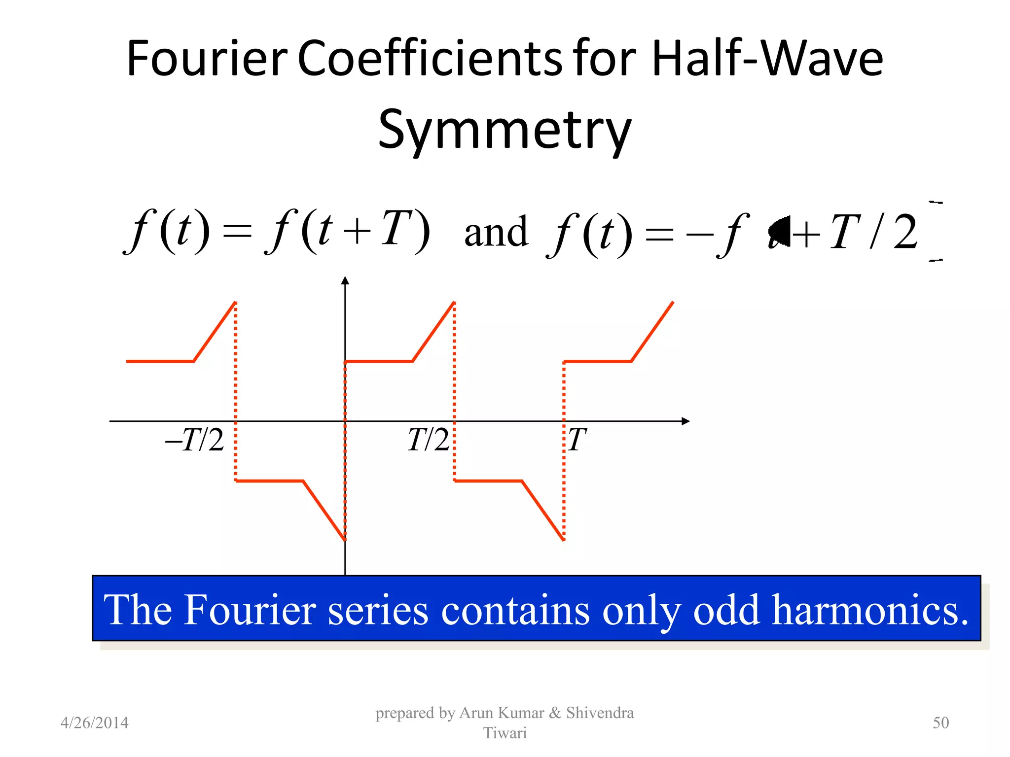
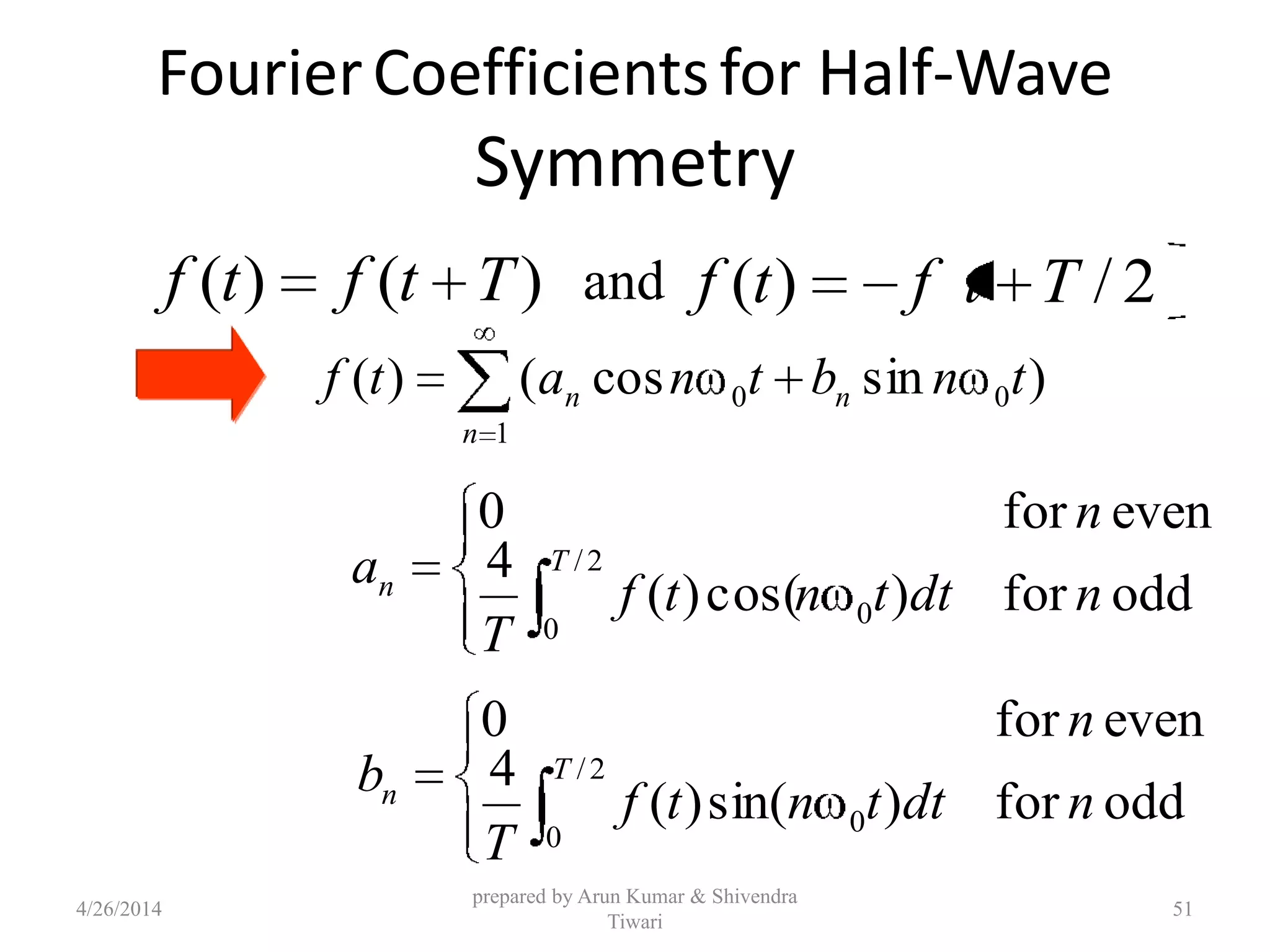
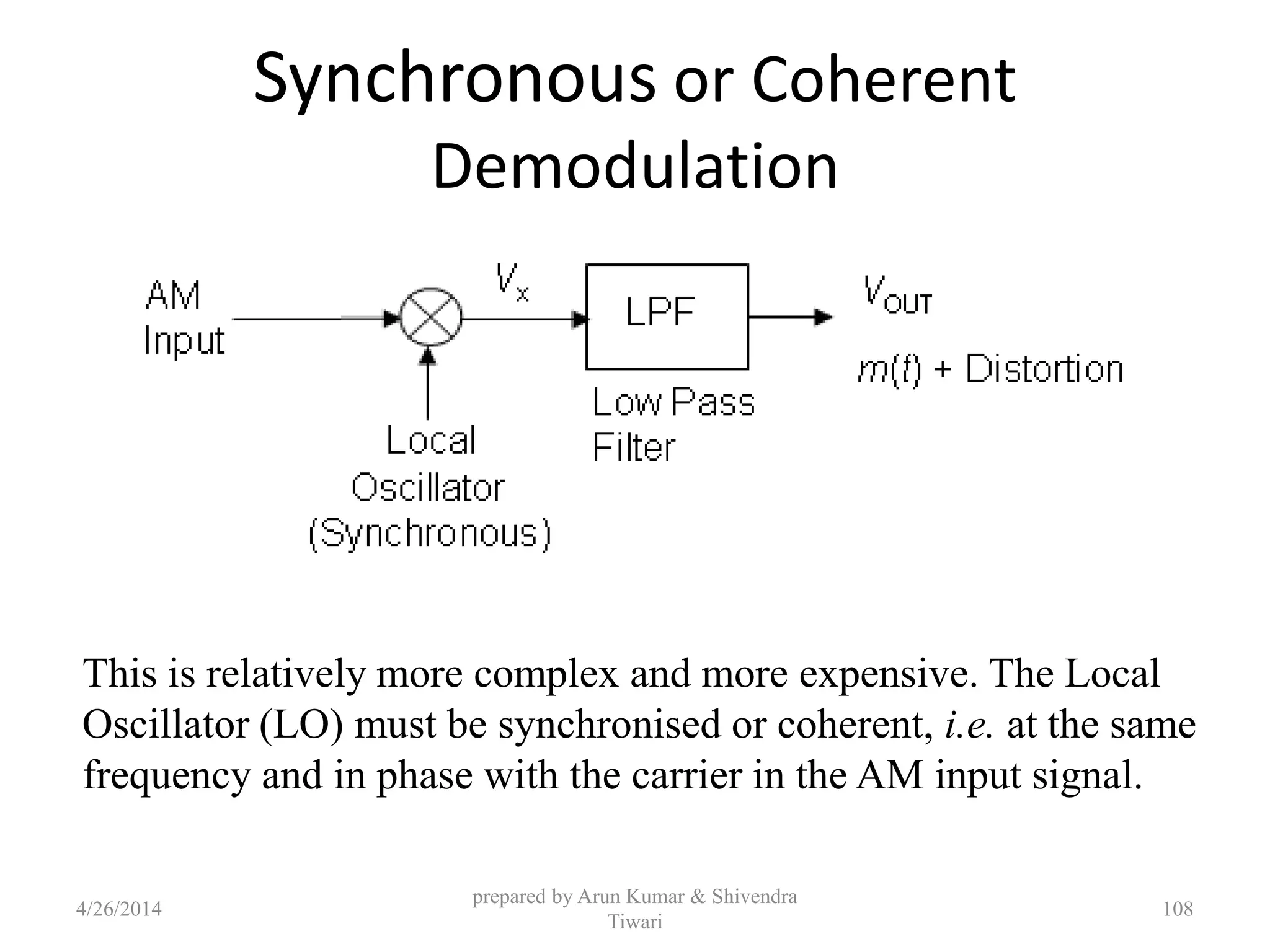
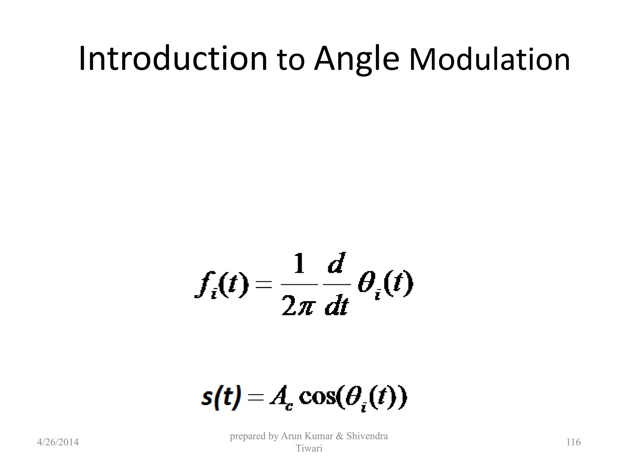
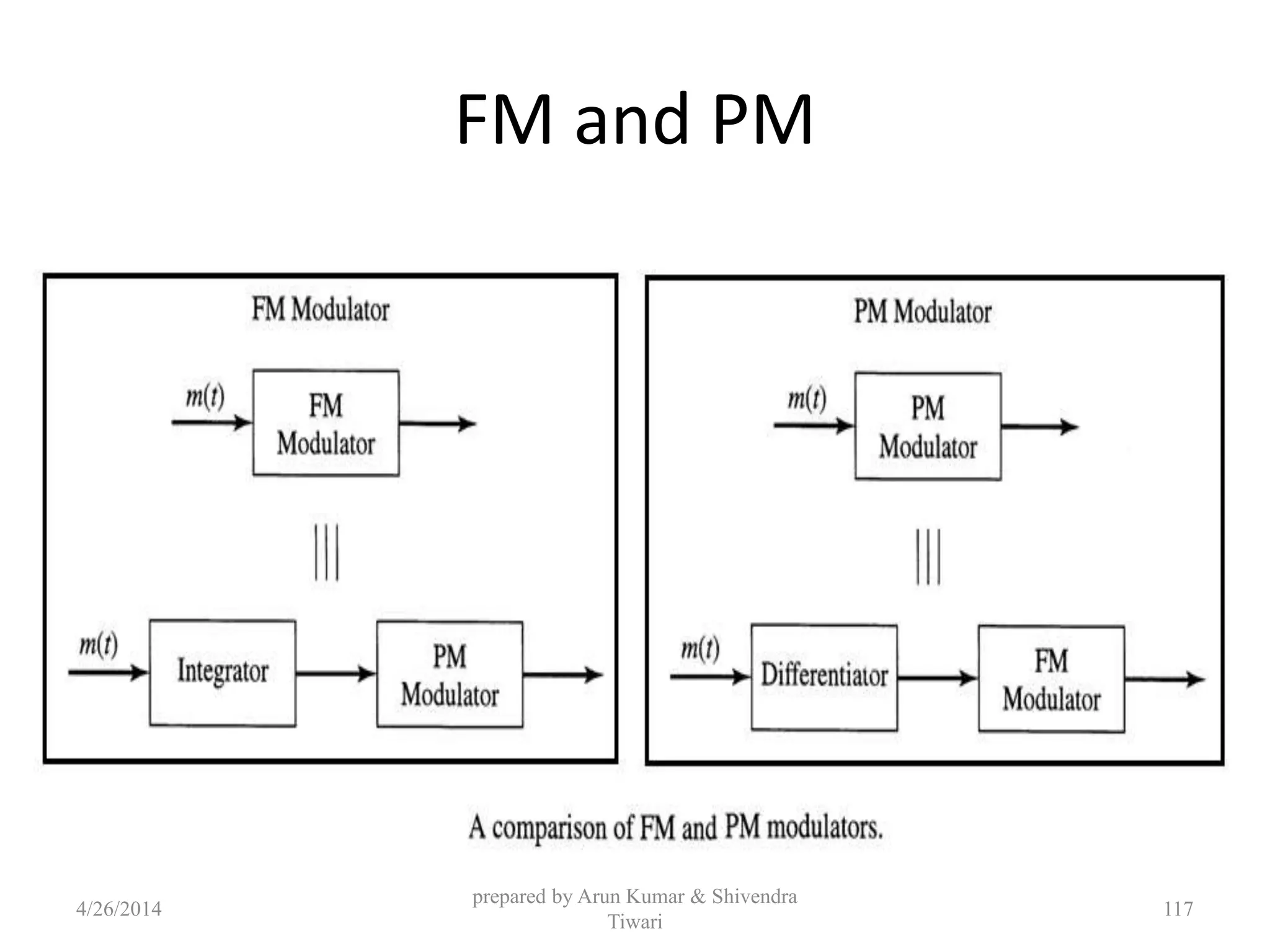
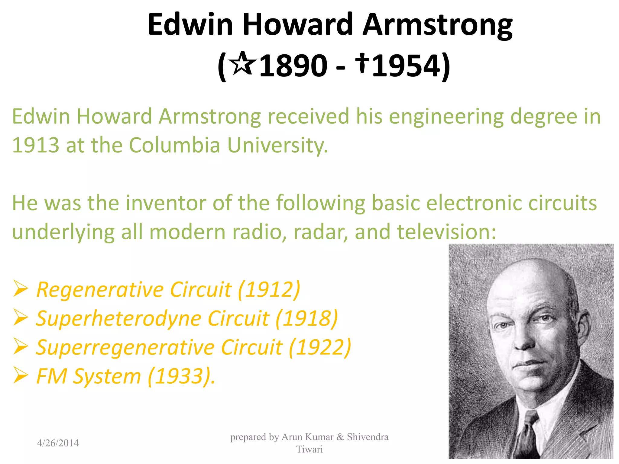
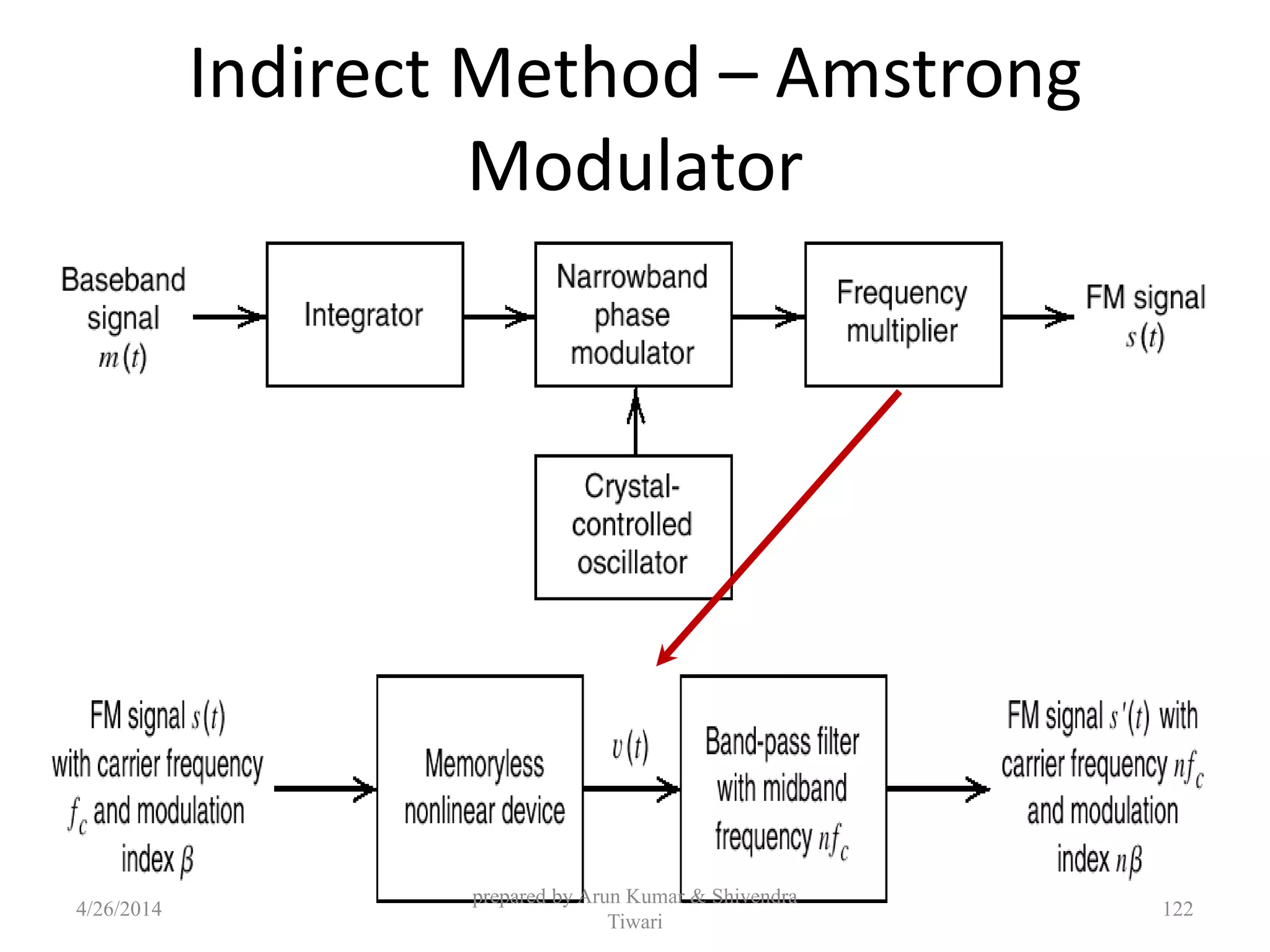
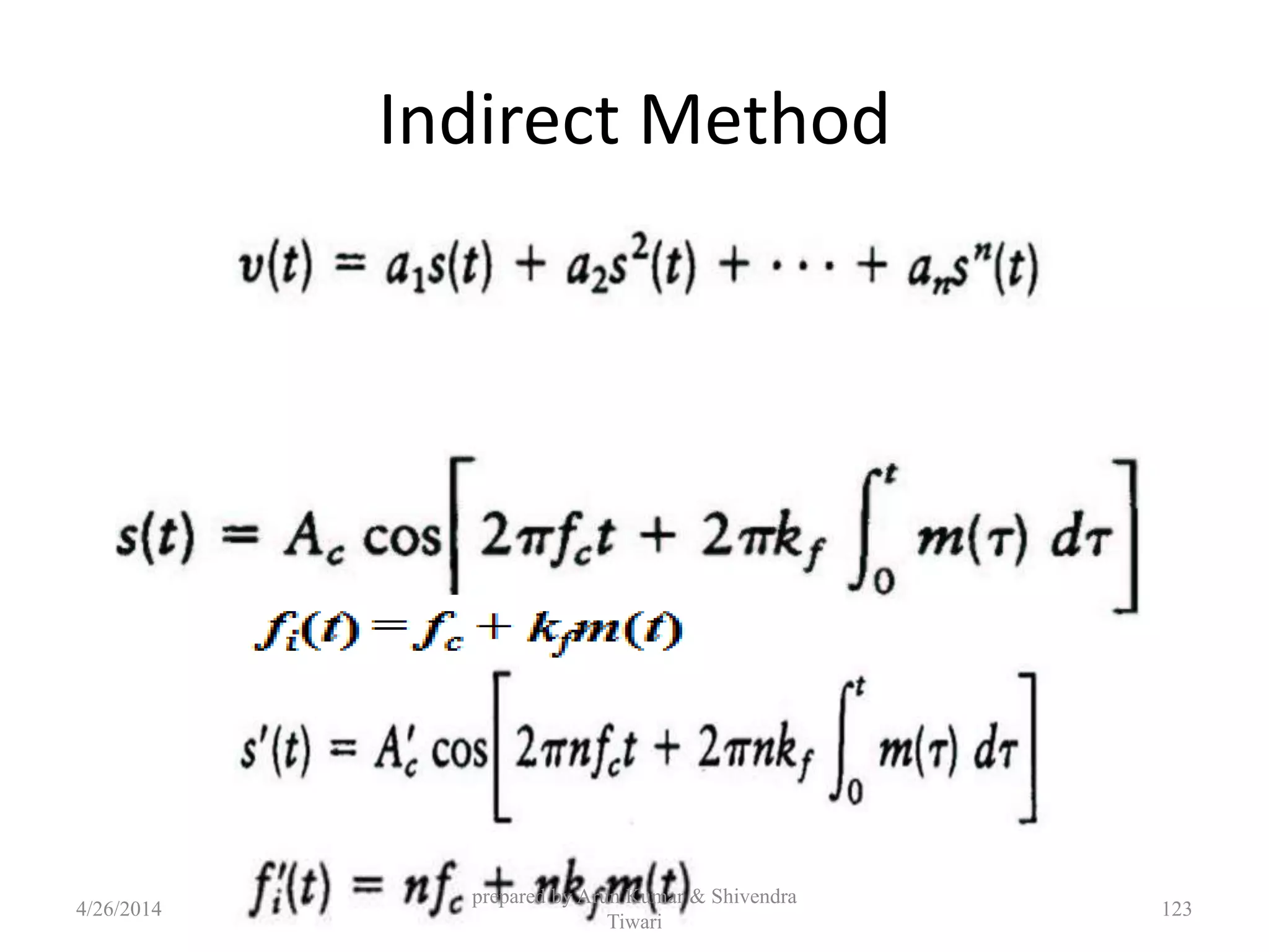
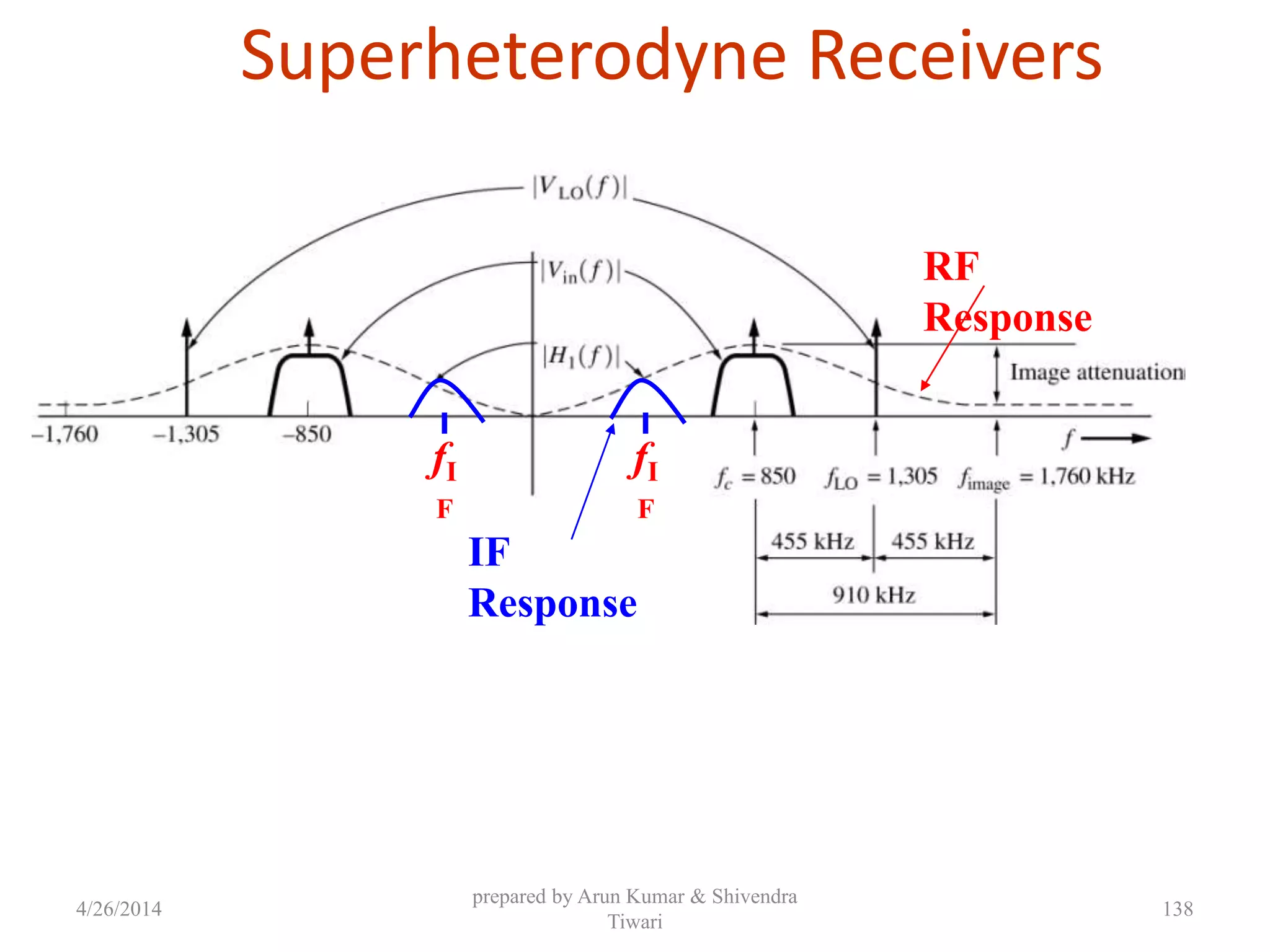
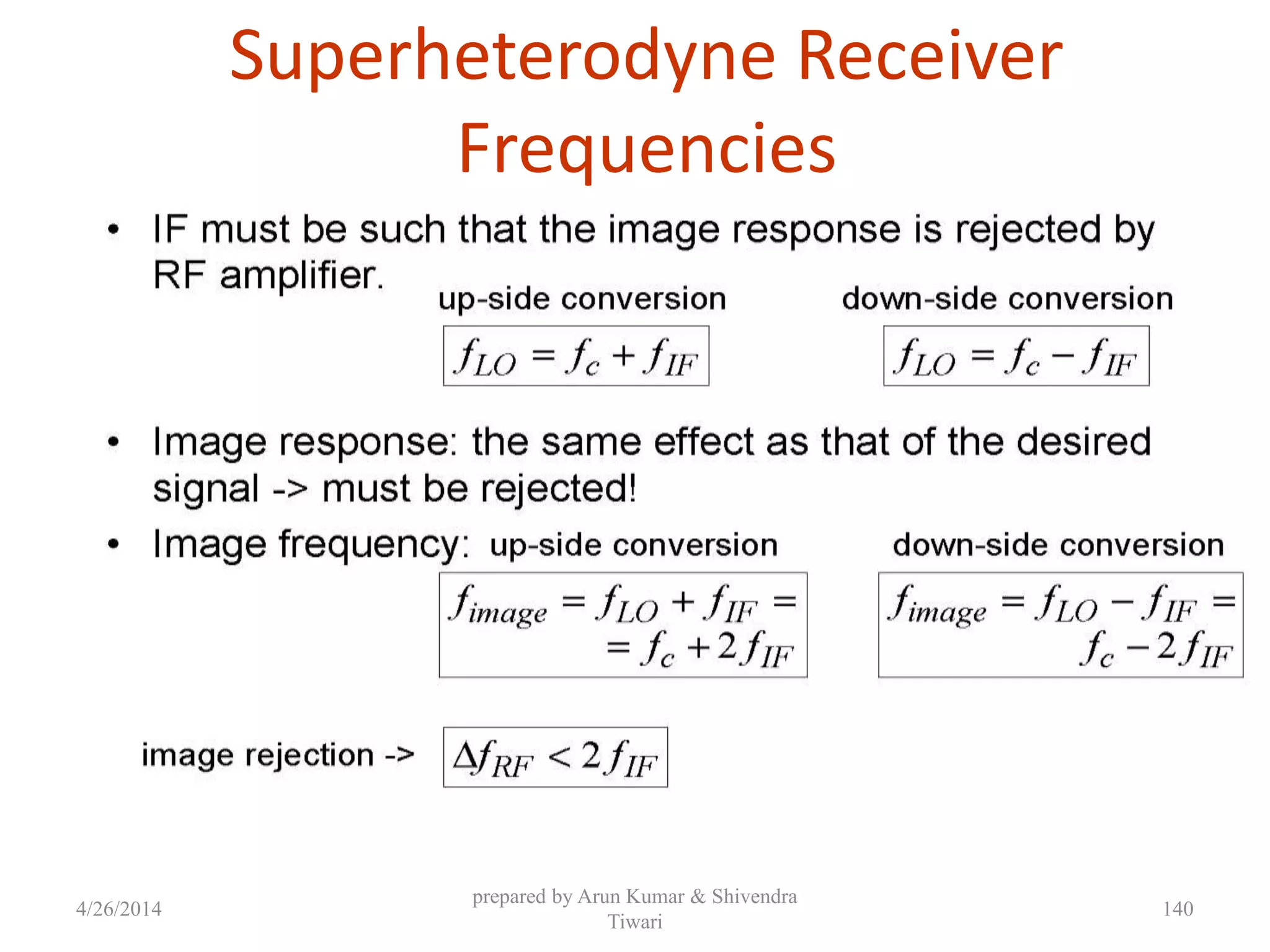
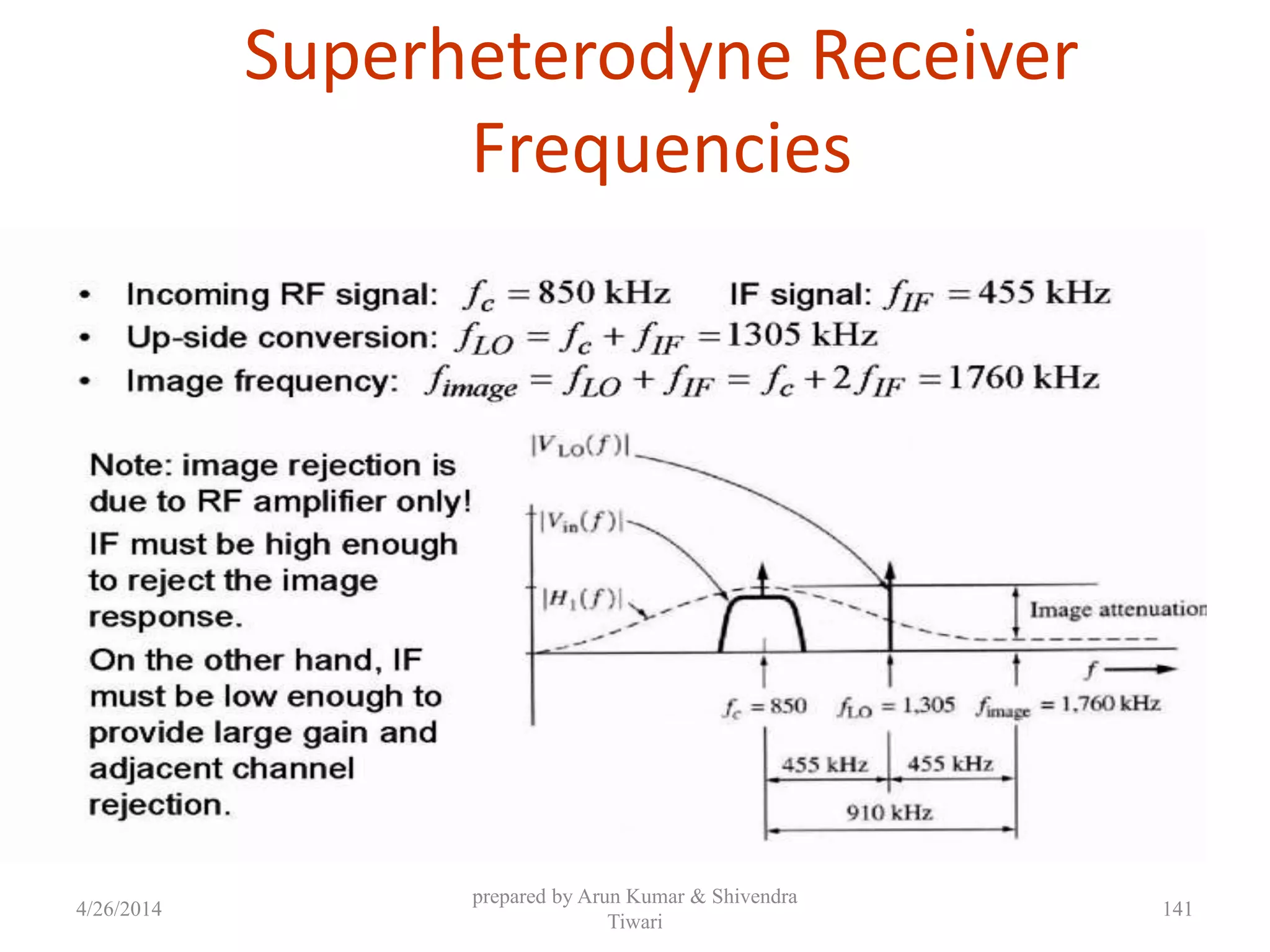
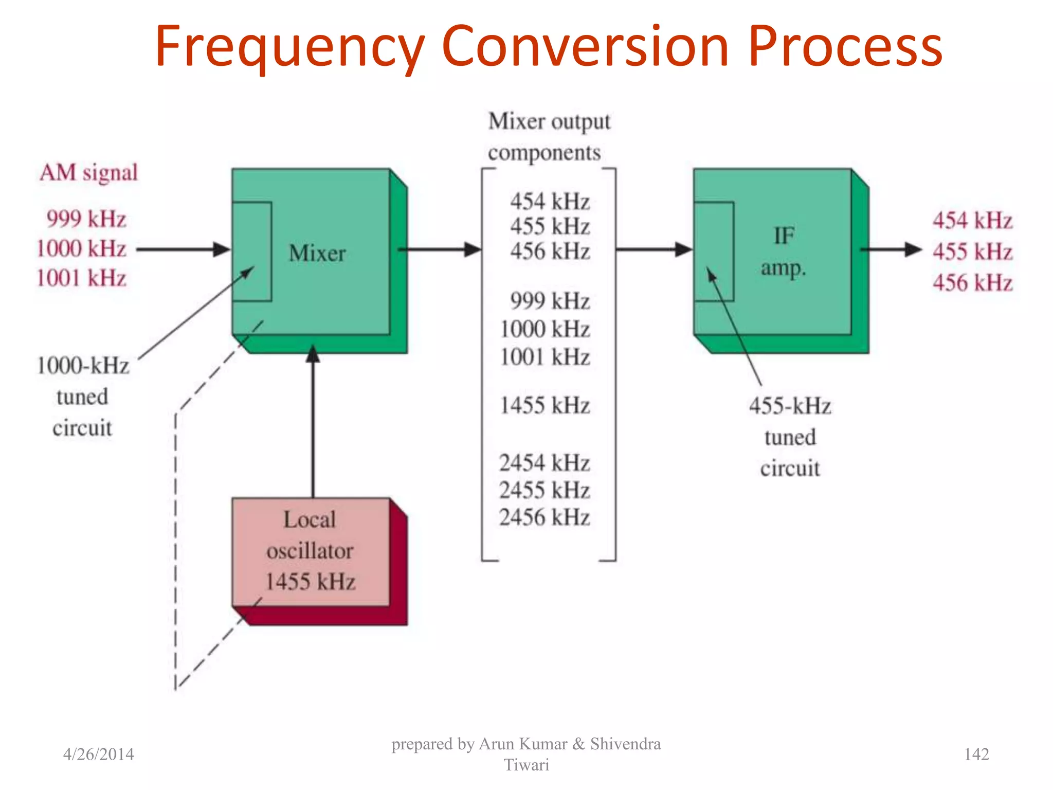
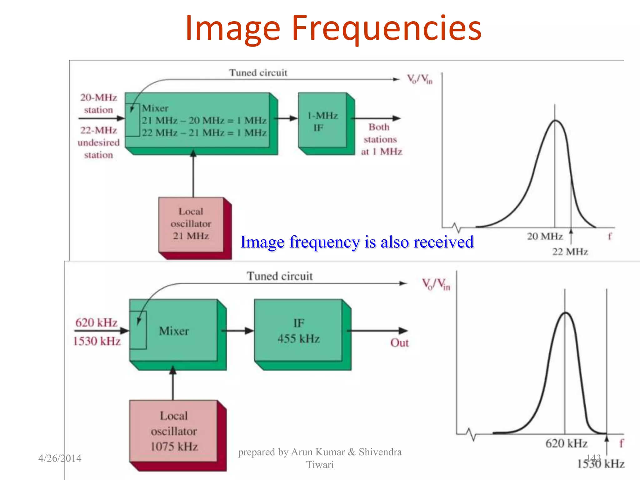
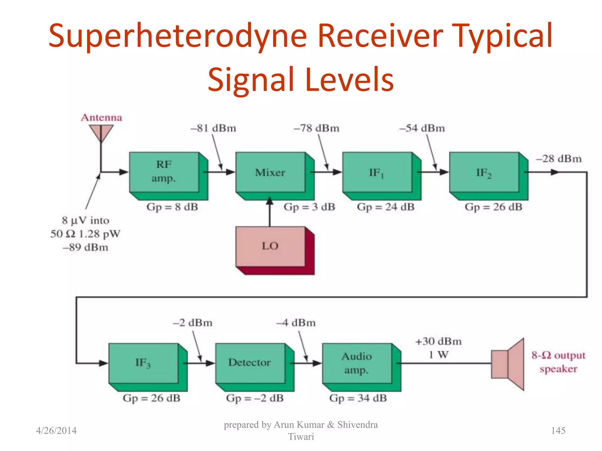
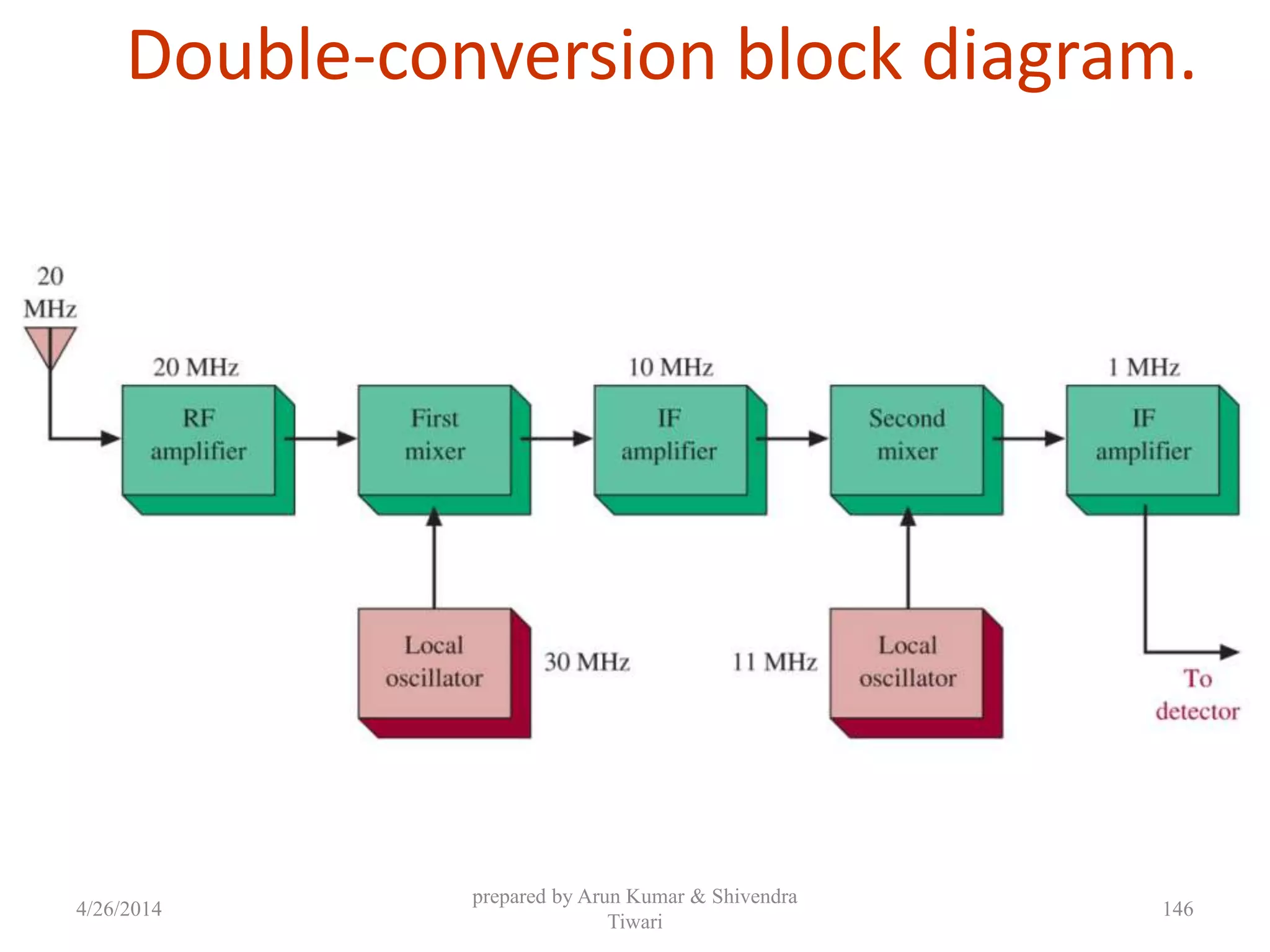
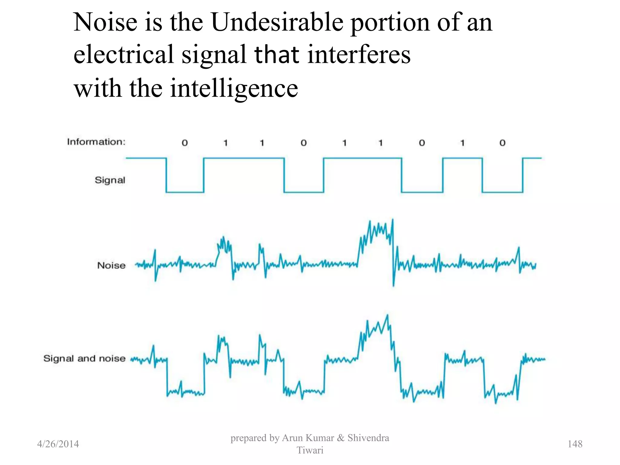
Downloaded 941 times
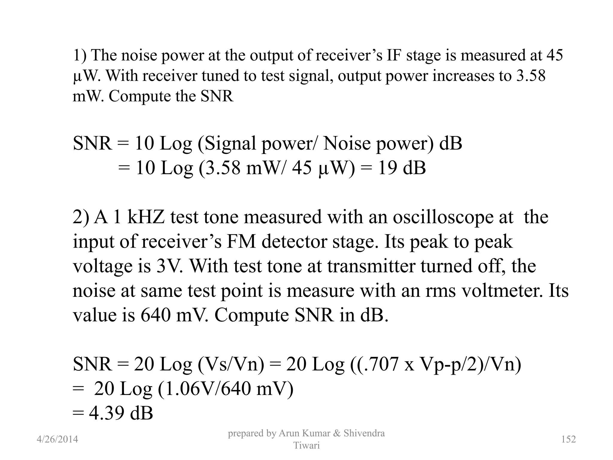
![Proof
dttntm
T
T
2/
2/
00 )cos()cos(
0
)]cos()[cos(
2
1
coscos
dttnmdttnm
T
T
T
T
2/
2/
0
2/
2/
0 ])cos[(
2
1
])cos[(
2
1
2/
2/0
0
2/
2/0
0
])sin[(
)(
1
2
1
])sin[(
)(
1
2
1 T
T
T
T
tnm
nm
tnm
nm
m n
])sin[(2
)(
1
2
1
])sin[(2
)(
1
2
1
00
nm
nm
nm
nm
0
04/26/2014
prepared by Arun Kumar & Shivendra
Tiwari
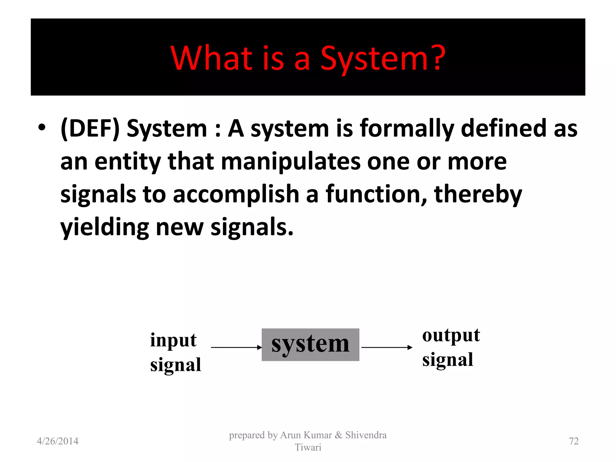
12](https://image.slidesharecdn.com/pptofanalogcommunication-140426051137-phpapp01/75/Ppt-of-analog-communication-12-2048.jpg)
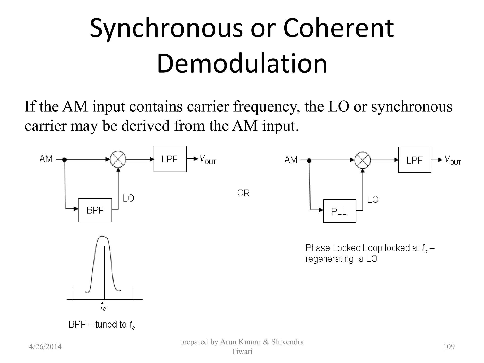
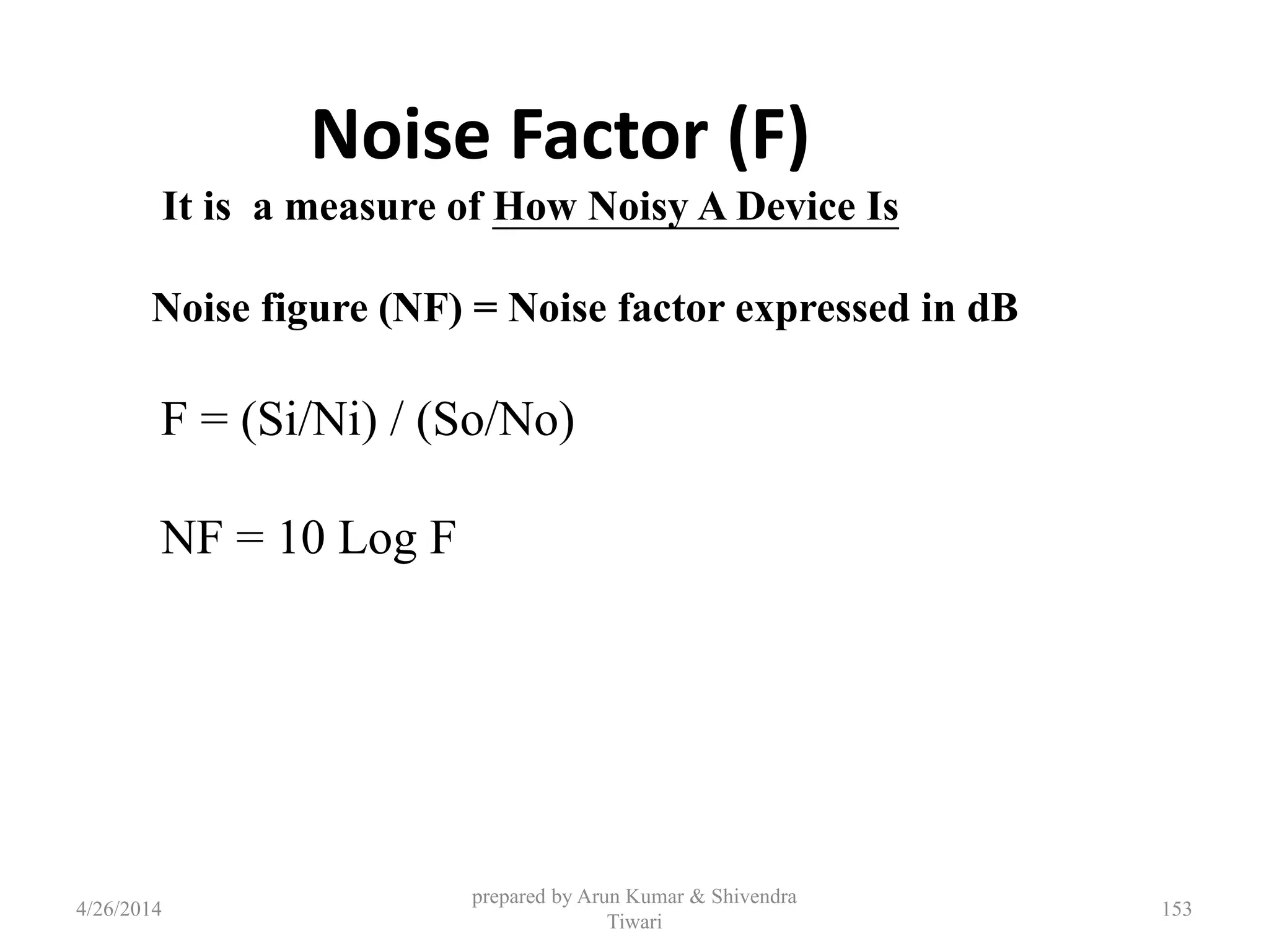
![Proof
dttntm
T
T
2/
2/
00 )cos()cos(
0
)]cos()[cos(
2
1
coscos
dttm
T
T
2/
2/
0
2
)(cos
2/
2/
0
0
2/
2/
]2sin
4
1
2
1
T
T
T
T
tm
m
t
m = n
2
T
]2cos1[
2
1
cos2
dttm
T
T
2/
2/
0 ]2cos1[
2
1
nmT
nm
dttntm
T
T 2/
0
)cos()cos(
2/
2/
00
4/26/2014
prepared by Arun Kumar & Shivendra
Tiwari
13](https://image.slidesharecdn.com/pptofanalogcommunication-140426051137-phpapp01/75/Ppt-of-analog-communication-13-2048.jpg)
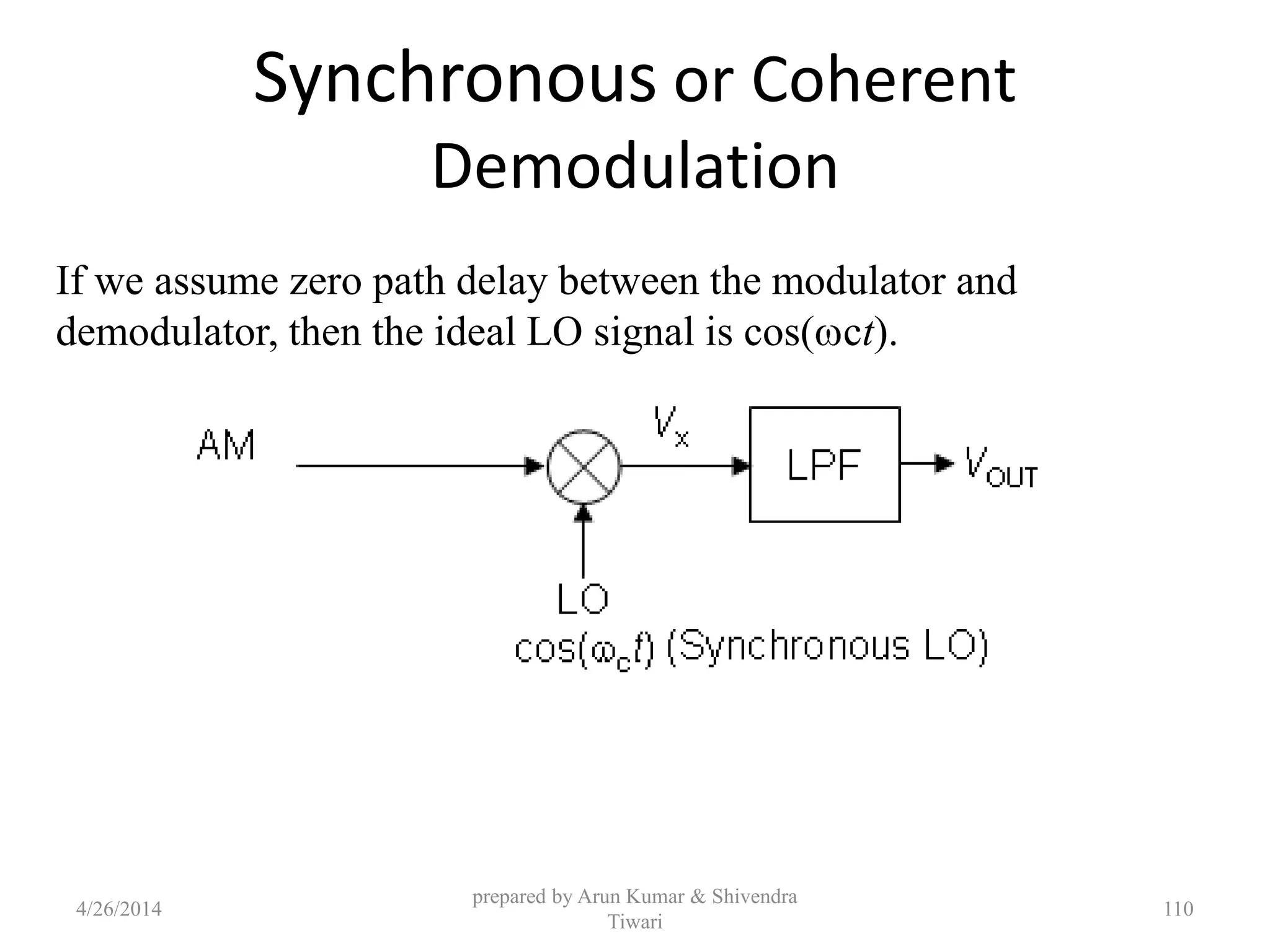
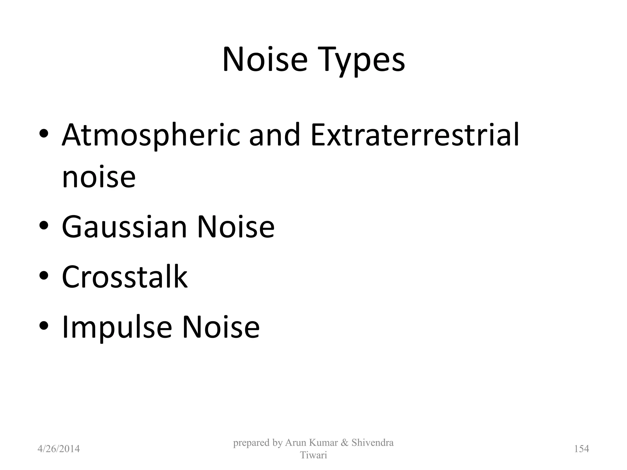
![Proof
dttntm
T
T
2/
2/
00 )cos()cos(
0
)]cos()[cos(
2
1
coscos
dttm
T
T
2/
2/
0
2
)(cos
2/
2/
0
0
2/
2/
]2sin
4
1
2
1
T
T
T
T
tm
m
t
m = n
2
T
]2cos1[
2
1
cos2
dttm
T
T
2/
2/
0 ]2cos1[
2
1
nmT
nm
dttntm
T
T 2/
0
)cos()cos(
2/
2/
00
4/26/2014
prepared by Arun Kumar & Shivendra
Tiwari
14](https://image.slidesharecdn.com/pptofanalogcommunication-140426051137-phpapp01/75/Ppt-of-analog-communication-14-2048.jpg)


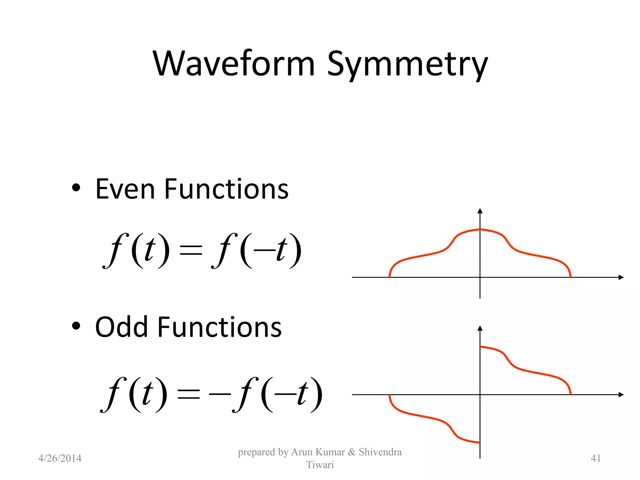
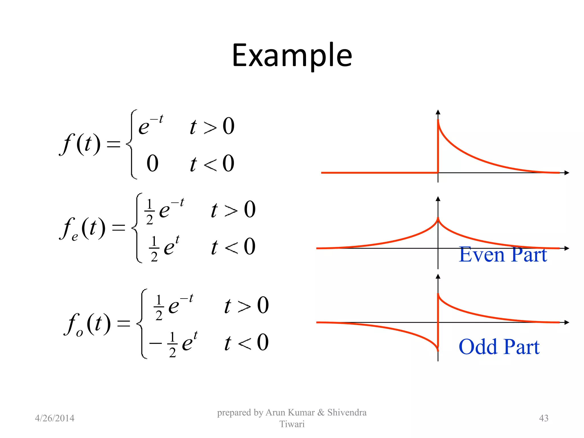
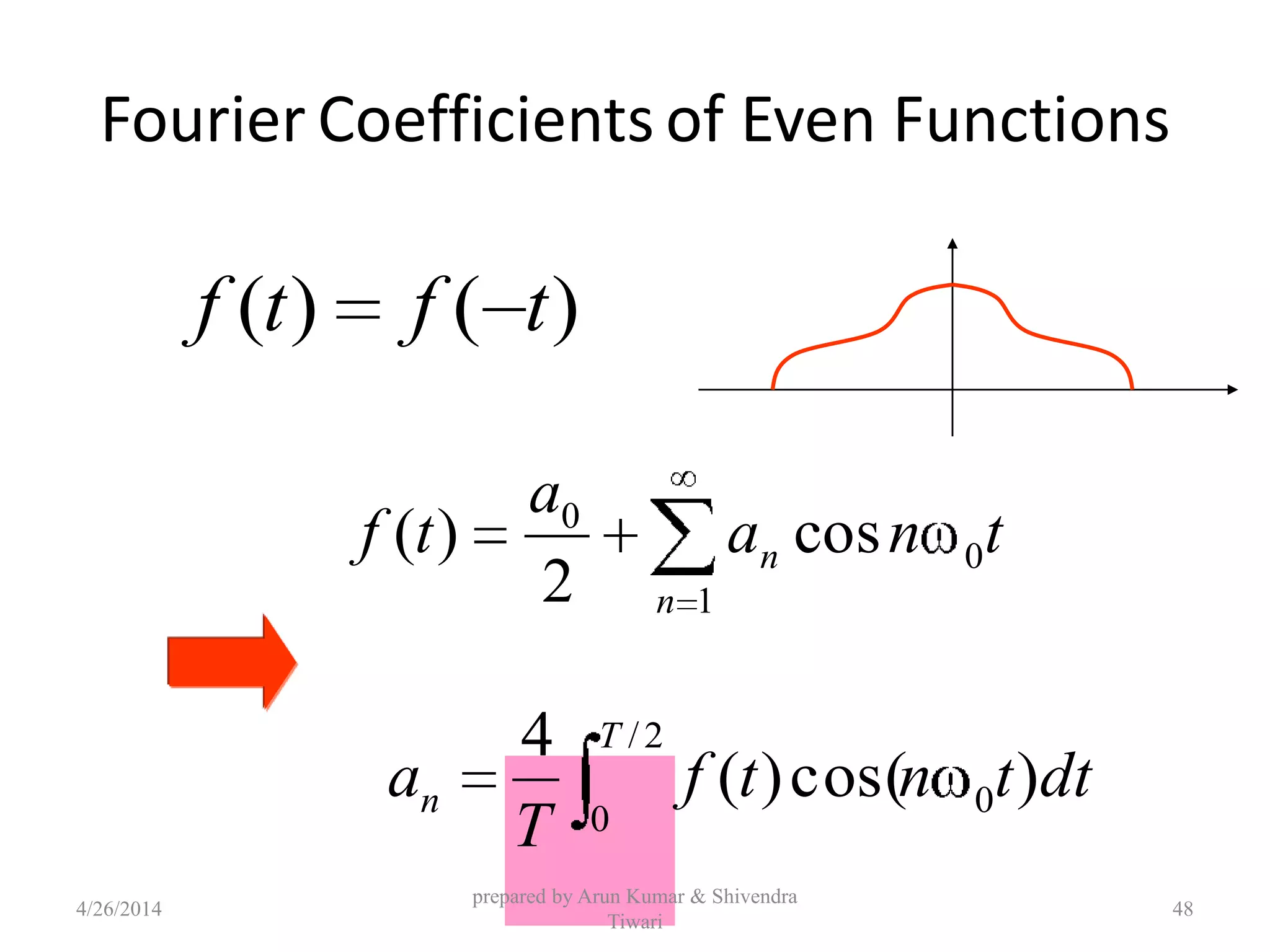
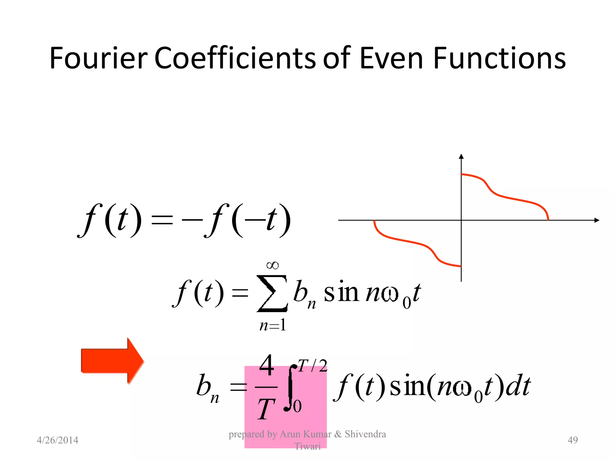
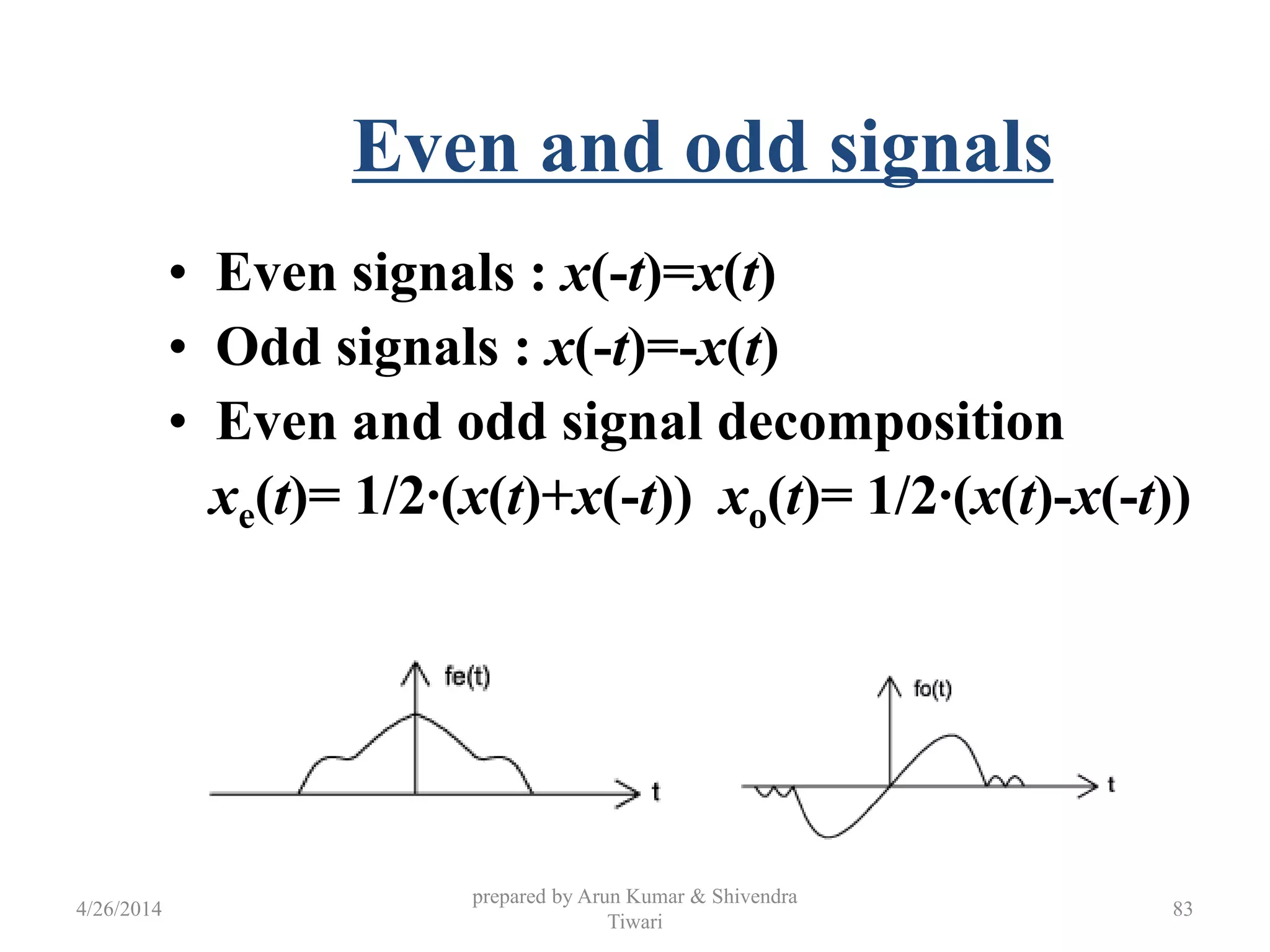
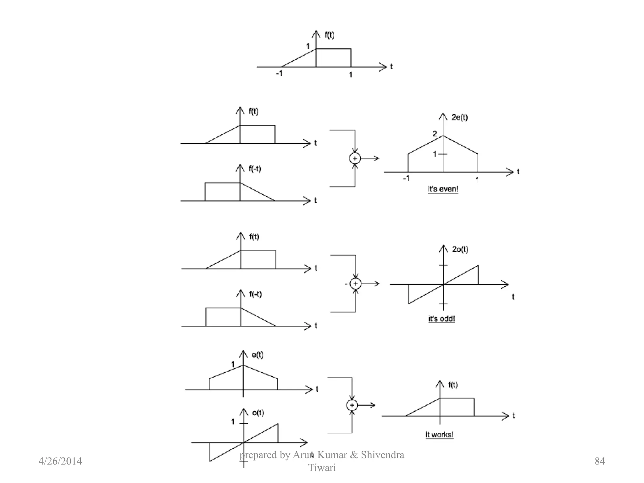
![Decomposition
• Any function f(t) can be expressed as the sum
of an even function fe(t) and an odd function
fo(t).
)()()( tftftf oe
)]()([)( 2
1
tftftfe
)]()([)( 2
1
tftftfo
Even Part
Odd Part
4/26/2014
prepared by Arun Kumar & Shivendra
Tiwari
42](https://image.slidesharecdn.com/pptofanalogcommunication-140426051137-phpapp01/75/Ppt-of-analog-communication-42-2048.jpg)

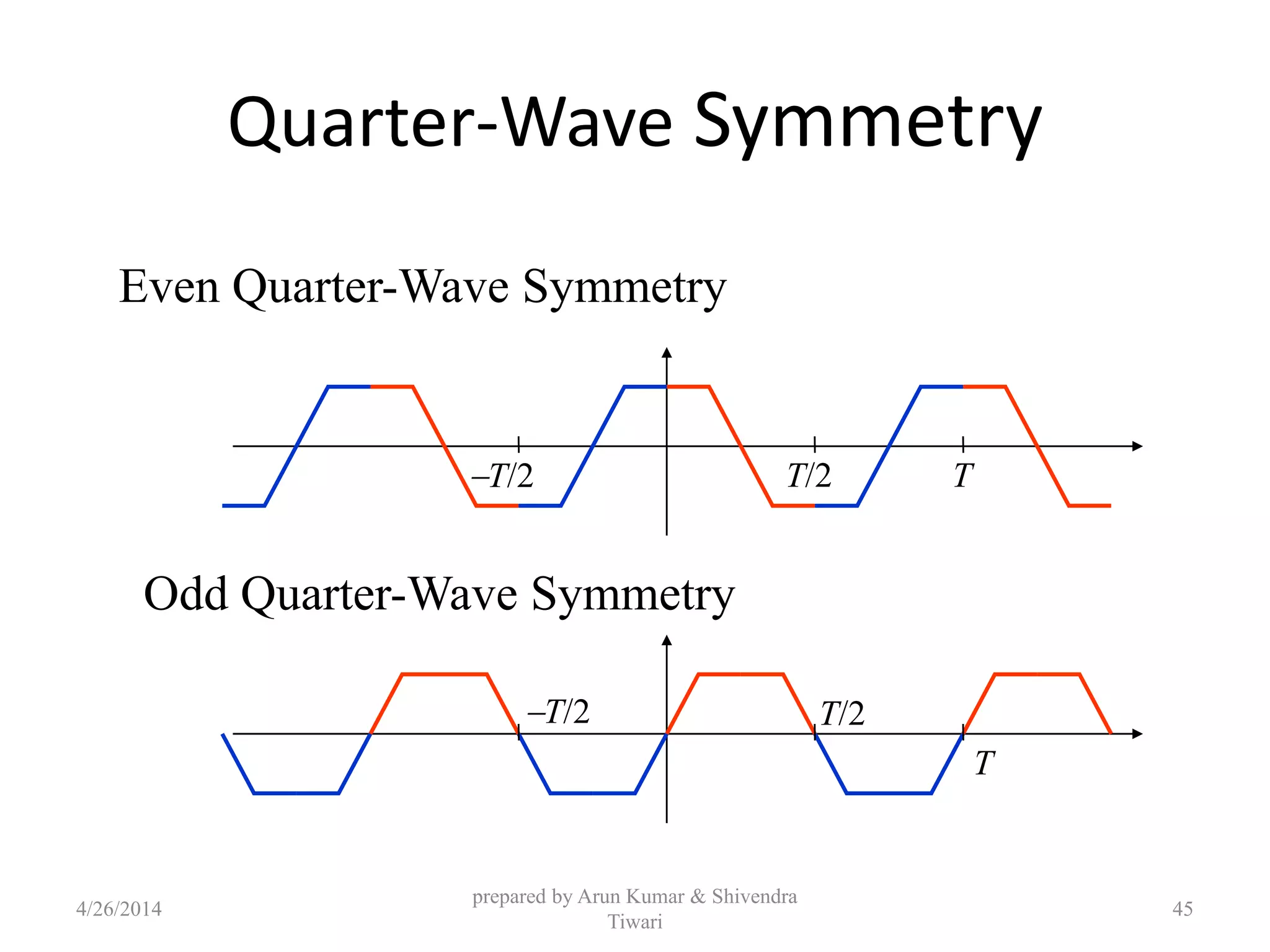

![Fourier Coefficients for
Even Quarter-Wave Symmetry
TT/2T/2
])12cos[()( 0
1
12 tnatf
n
n
4/
0
012 ])12cos[()(
8 T
n dttntf
T
a
4/26/2014
prepared by Arun Kumar & Shivendra
Tiwari
52](https://image.slidesharecdn.com/pptofanalogcommunication-140426051137-phpapp01/75/Ppt-of-analog-communication-52-2048.jpg)


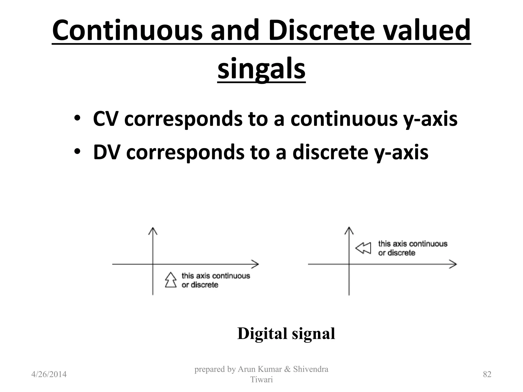
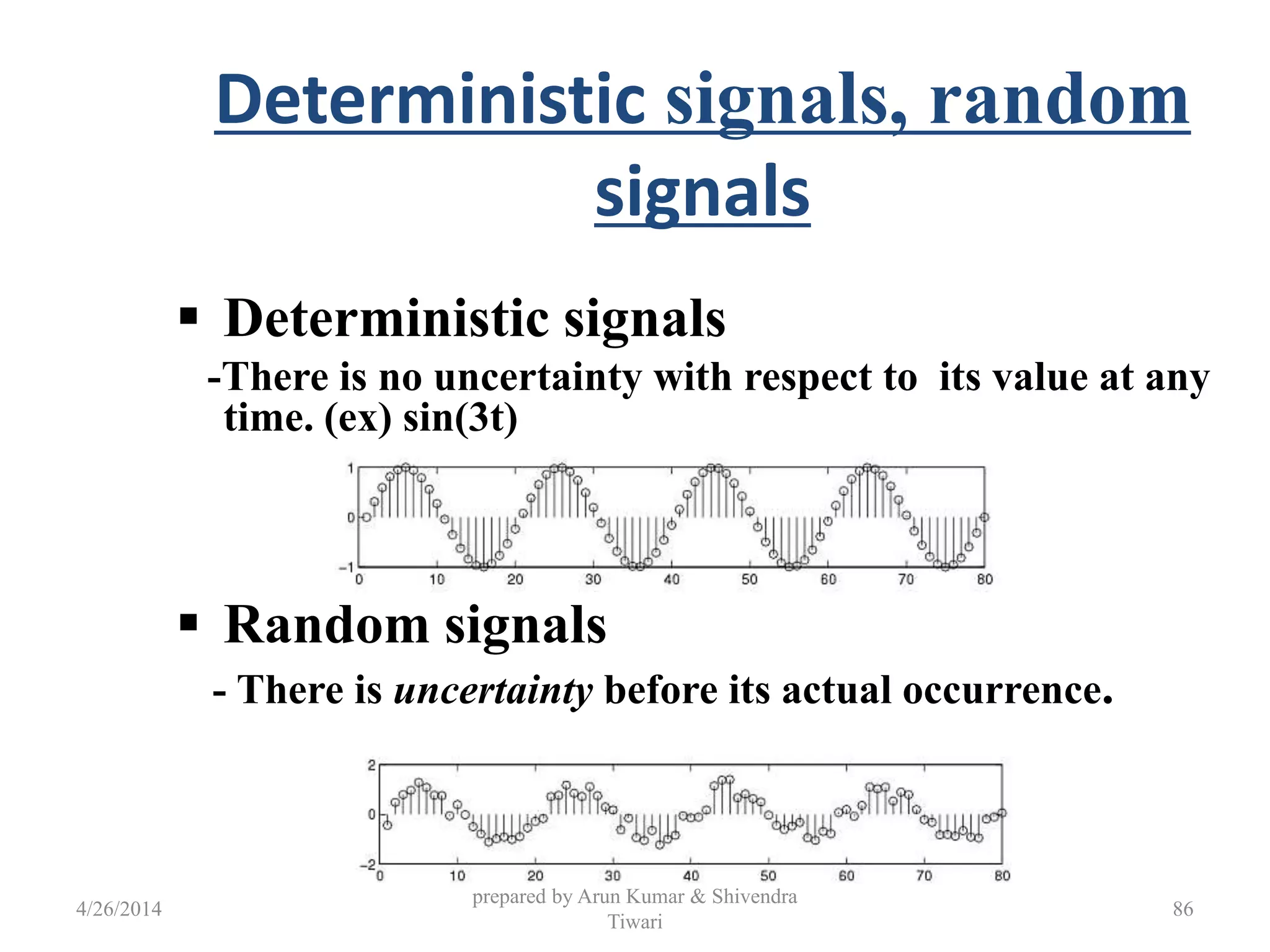
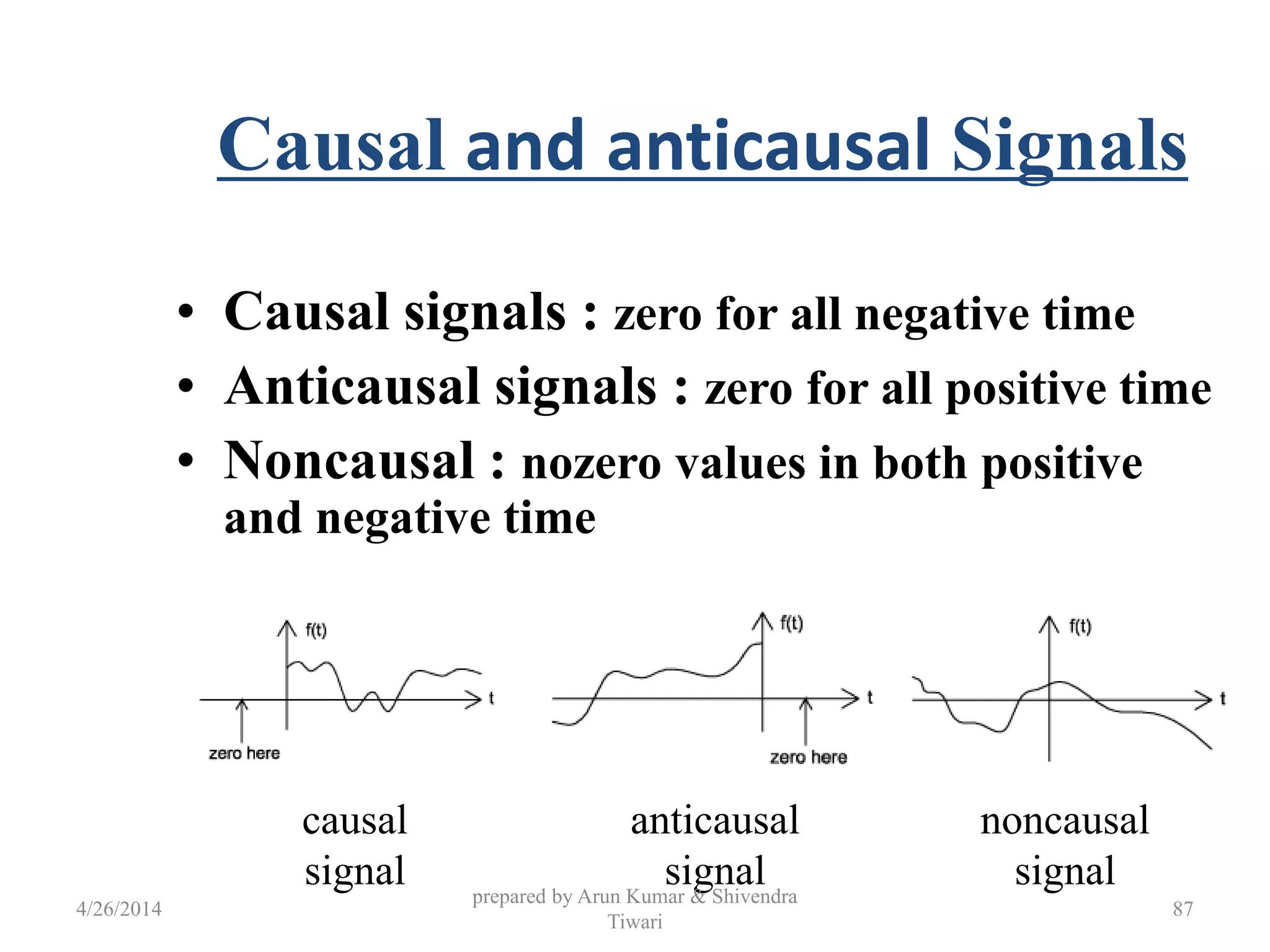
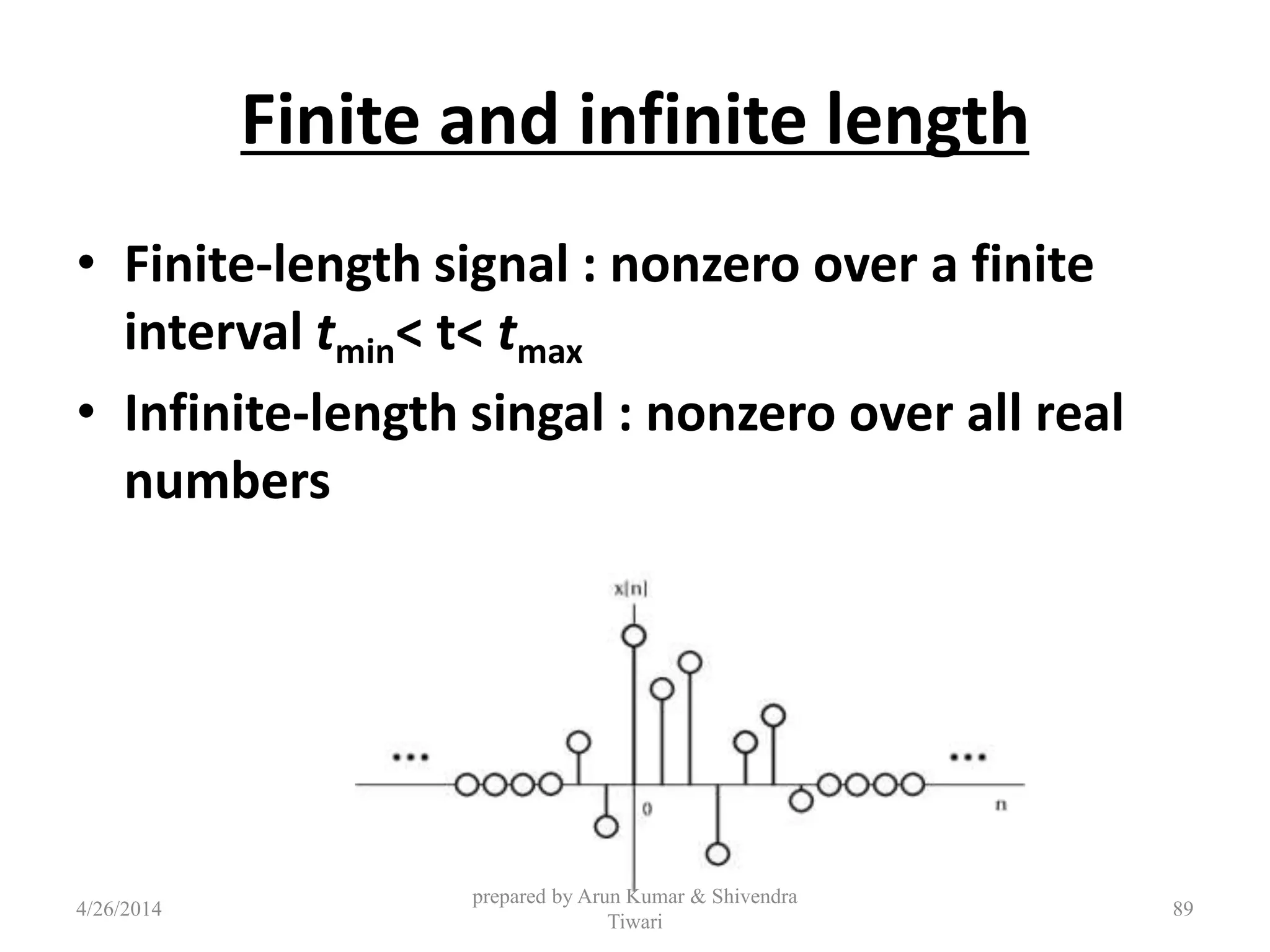
![Continuous and discrete-time
signals
• Continuous signal
- It is defined for all time t : x(t)
• Discrete-time signal
- It is defined only at discrete instants of time :
x[n]=x(nT)
4/26/2014
prepared by Arun Kumar & Shivendra
Tiwari
81](https://image.slidesharecdn.com/pptofanalogcommunication-140426051137-phpapp01/75/Ppt-of-analog-communication-81-2048.jpg)


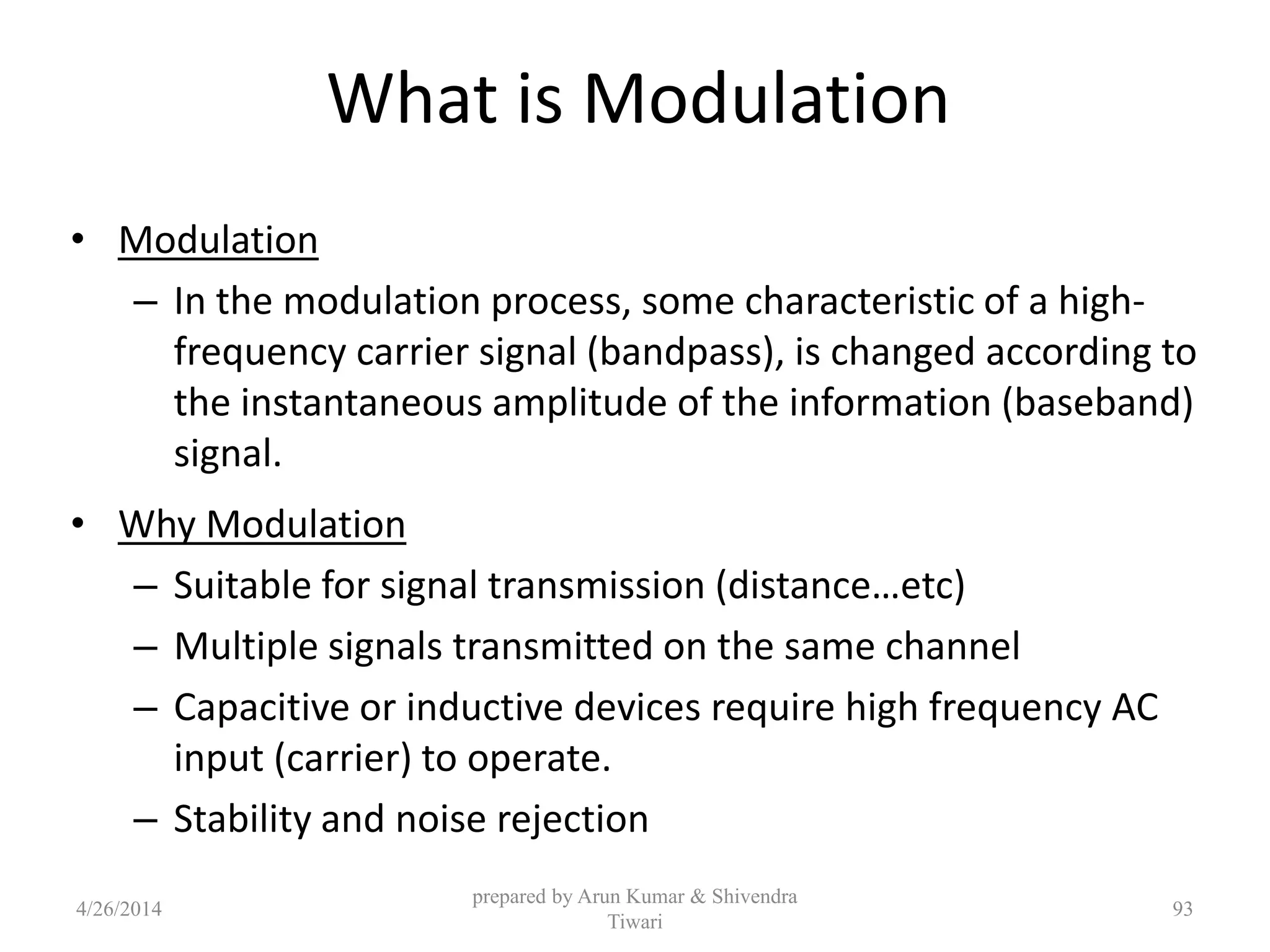
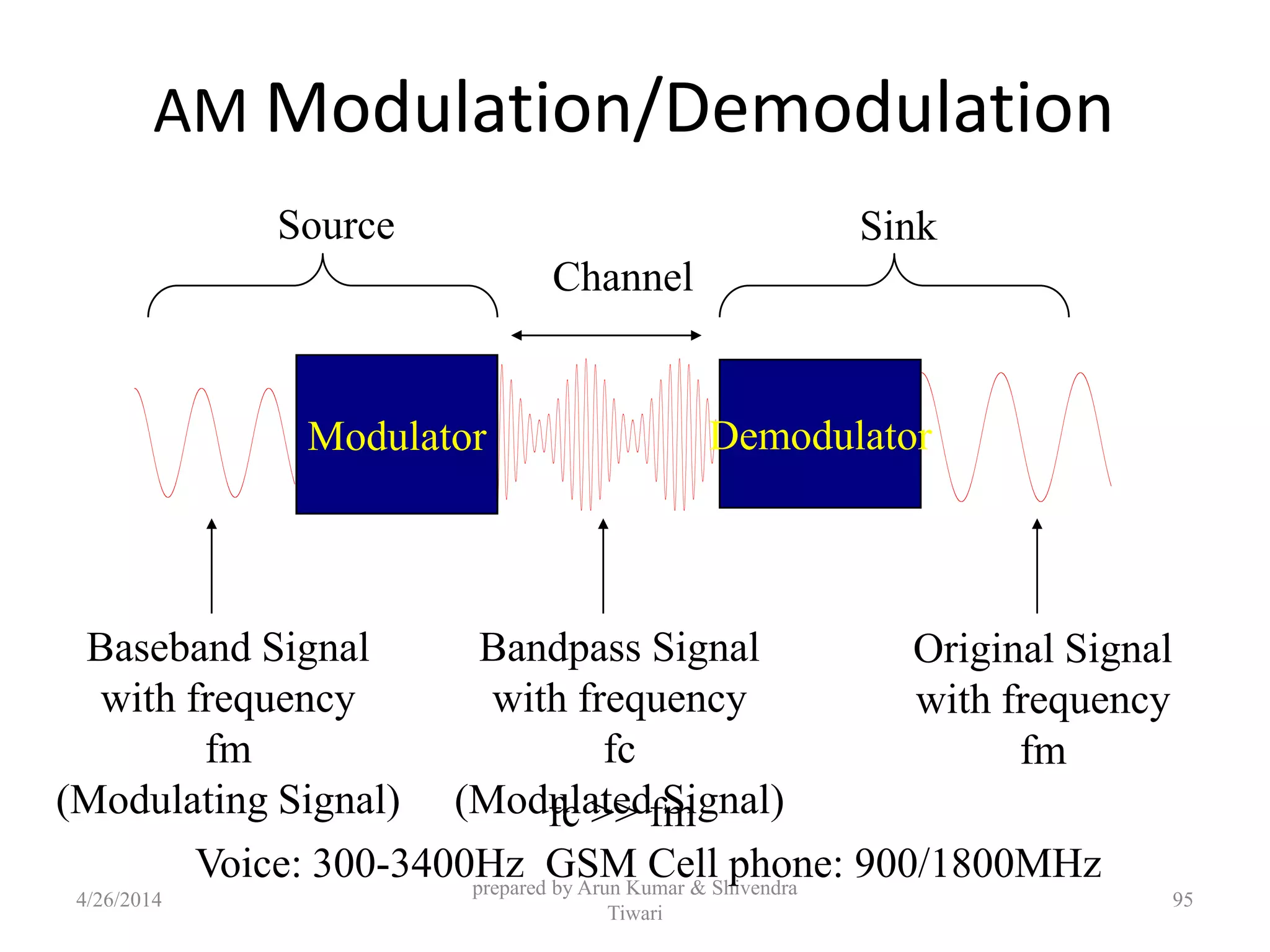
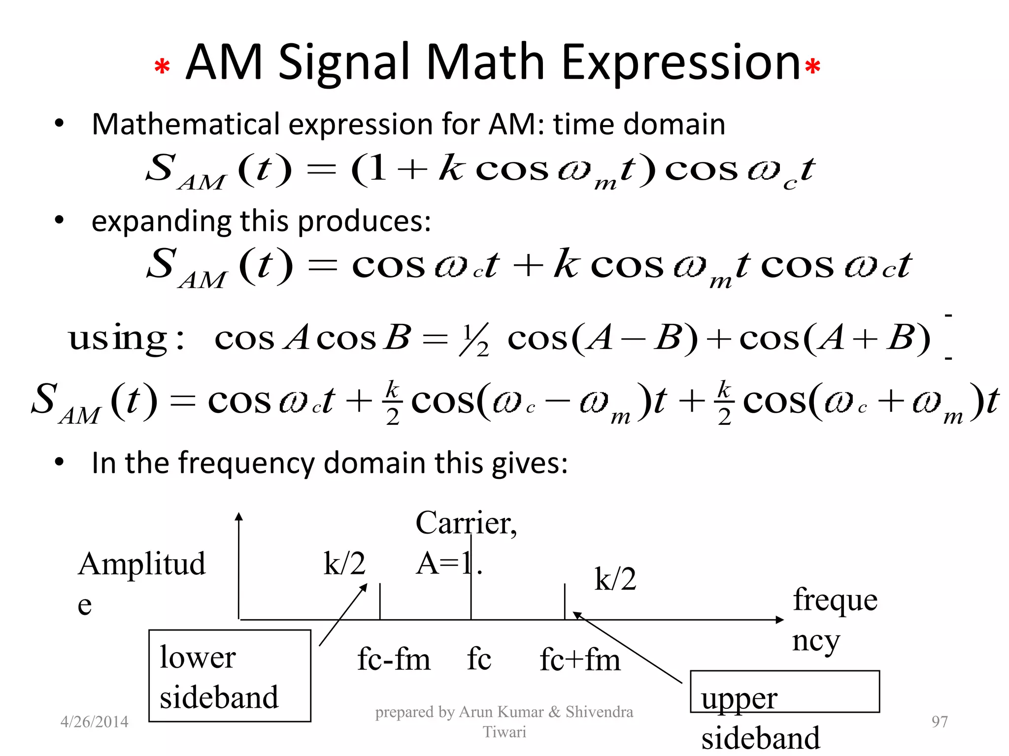
![Amplitude Modulation
• The amplitude of high-carrier signal is varied
according to the instantaneous amplitude of the
modulating message signal m(t).
Carrier Signal: or
Modulating Message Signal: or
The AM Signal:
cos(2 ) cos( )
( ): cos(2 ) cos( )
( ) [ ( )]cos(2 )
c c
m m
AM c c
f t t
m t f t t
s t A m t f t
prepared by Arun Kumar & Shivendra
Tiwari
4/26/2014 96](https://image.slidesharecdn.com/pptofanalogcommunication-140426051137-phpapp01/75/Ppt-of-analog-communication-96-2048.jpg)
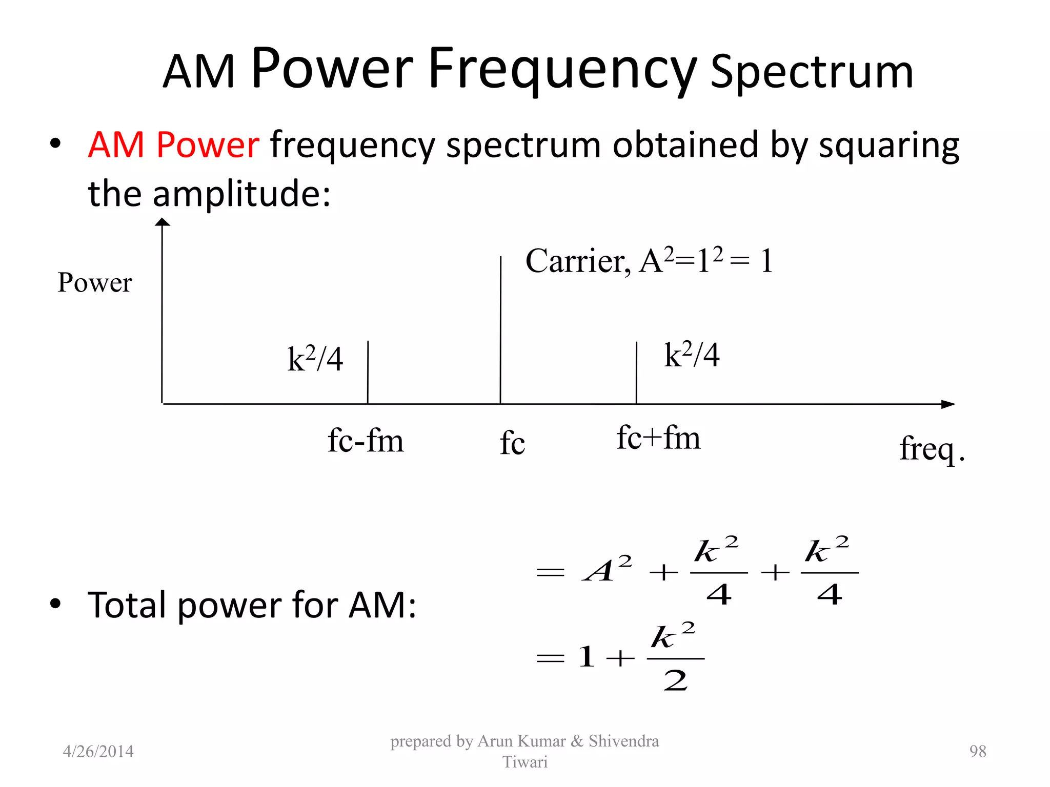
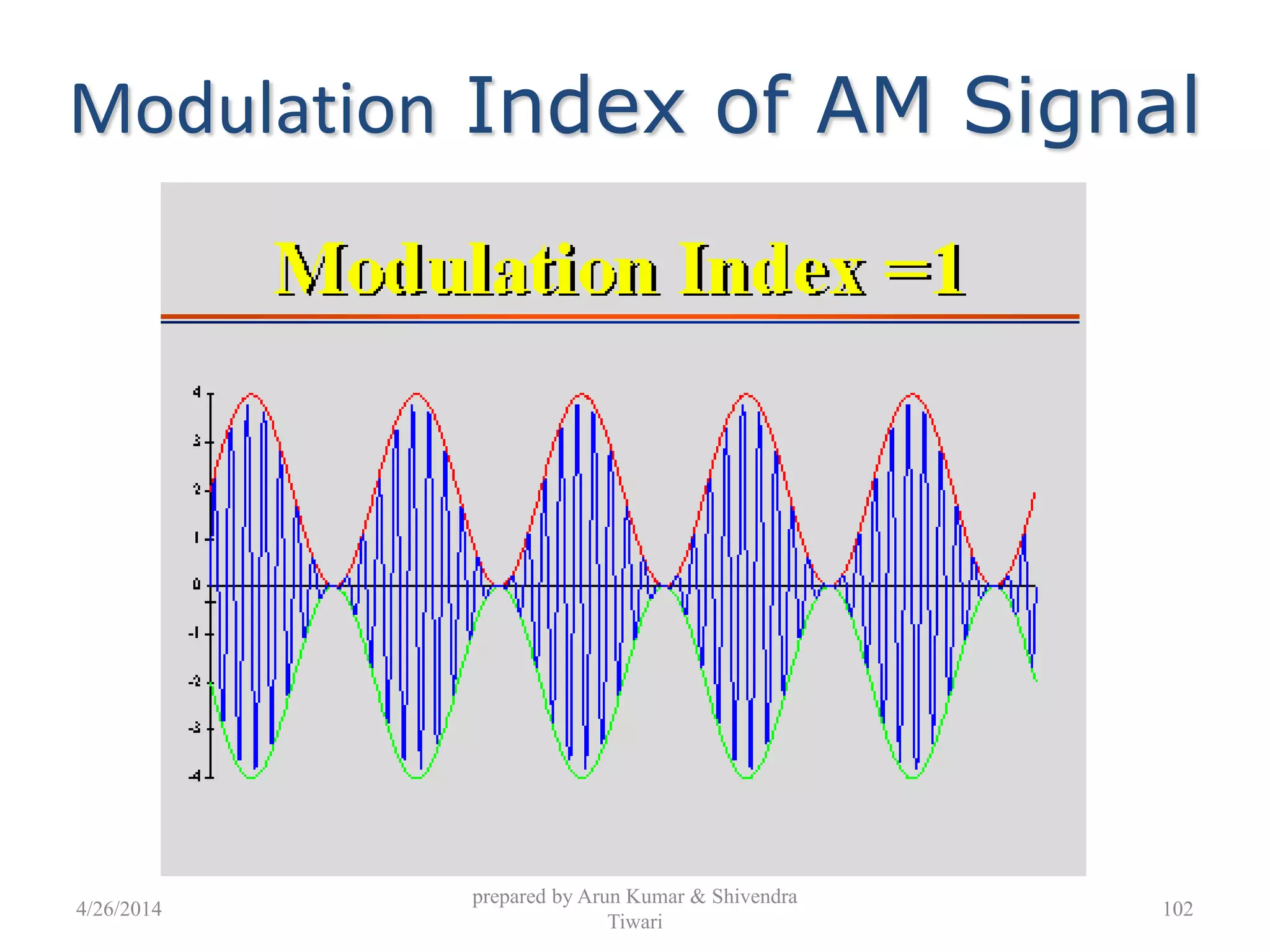
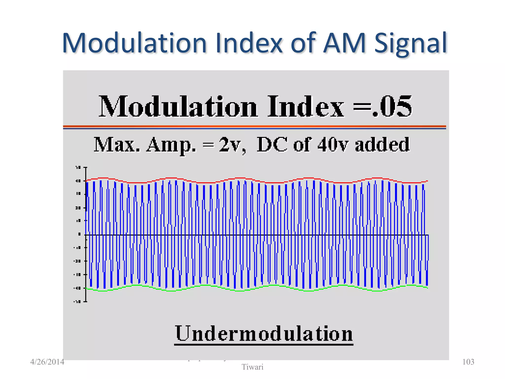
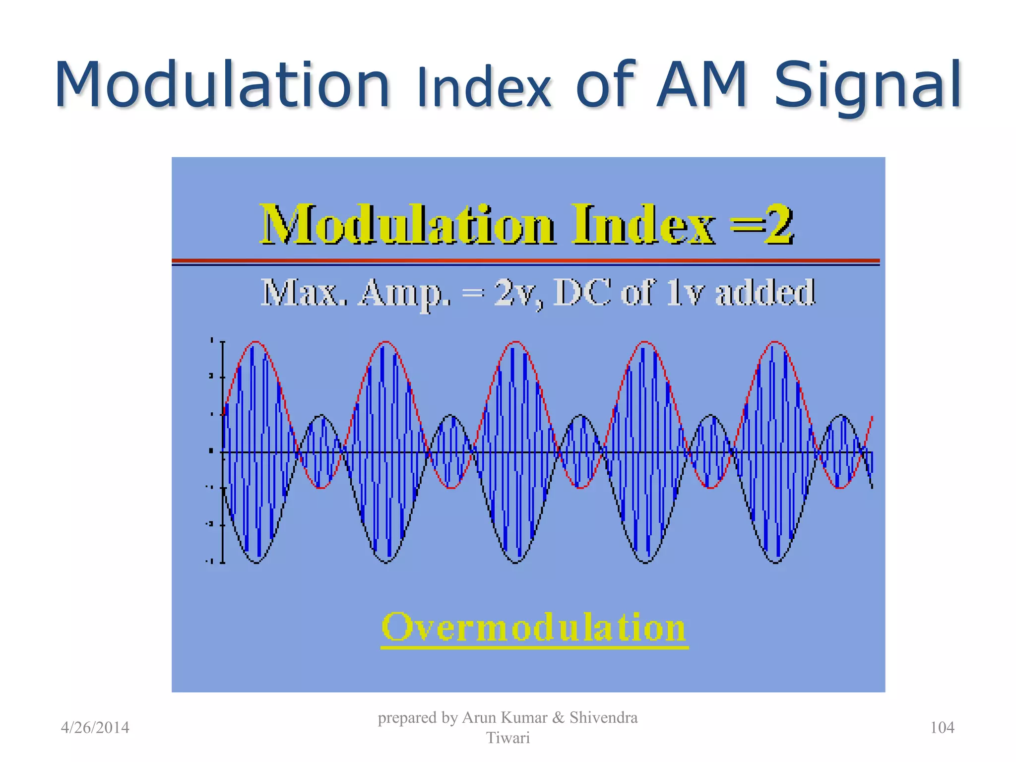
![Modulation Index of AM Signal
m
c
A
k
A
)2cos()( tfAtm mm
Carrier Signal: cos(2 ) DC:c Cf t A
Modulated Signal: ( ) [ cos(2 )]cos(2 )
[1 cos(2 )]cos(2 )
AM c m m c
c m c
S t A A f t f t
A k f t f t
prepared by Arun Kumar & Shivendra
Tiwari
For a sinusoidal message signal
Modulation Index is defined as:
Modulation index k is a measure of the extent to
which a carrier voltage is varied by the modulating
signal. When k=0 no modulation, when k=1 100%
modulation, when k>1 over modulation.
4/26/2014 101](https://image.slidesharecdn.com/pptofanalogcommunication-140426051137-phpapp01/75/Ppt-of-analog-communication-101-2048.jpg)


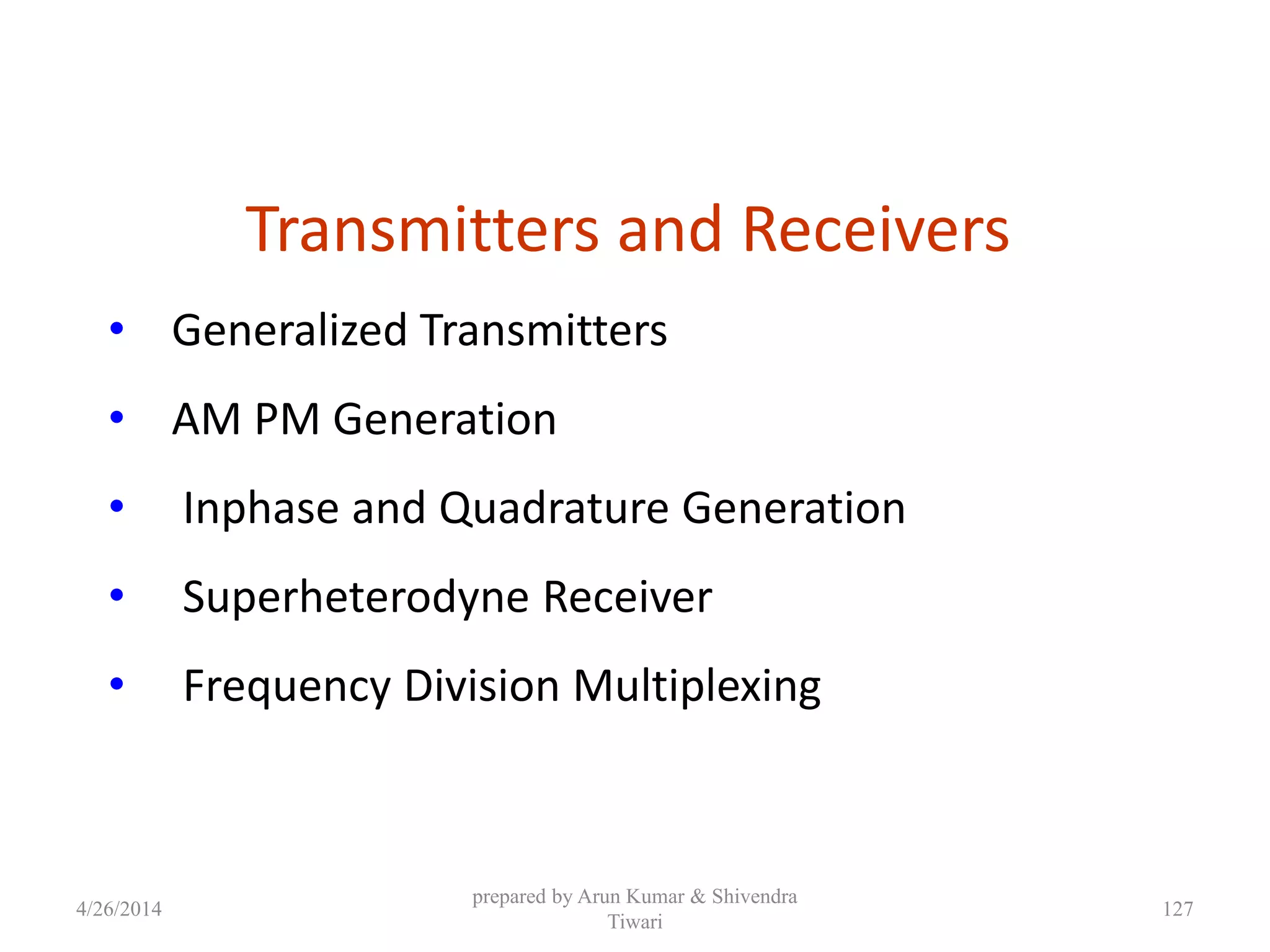
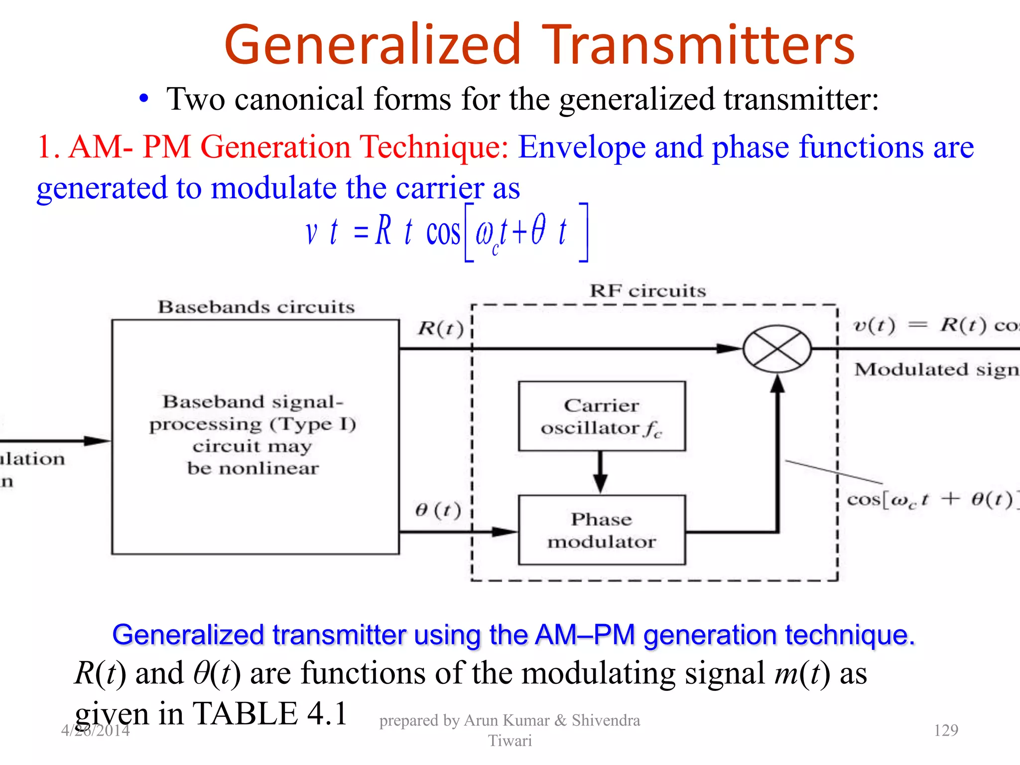
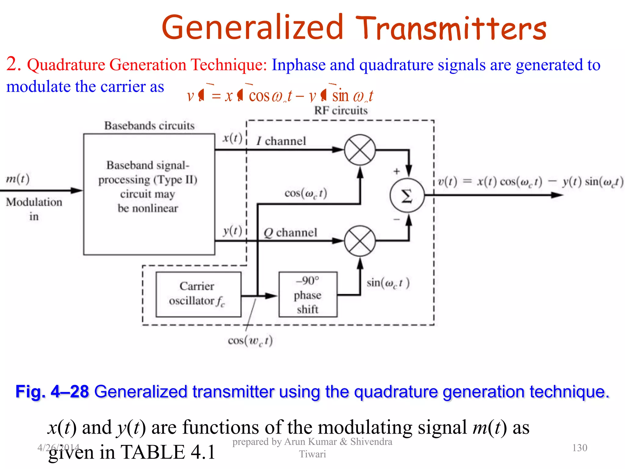
![Generalized Transmitters
Re cos
cos sin
Where
cj t
c
c c
j t
v t g t e R t t t
v t x t t y t t
g t R t e x t jy t
Any type of modulated signal can be represented by
The complex envelope g(t) is a function of the
modulating signal m(t)
Transmitter
Modulating
signal
Modulated
signal
Example:
( )
Type of Modulation g(m)
AM : [1 ( )]
PM : p
c
jD m t
c
A m t
A e
4/26/2014
prepared by Arun Kumar & Shivendra
Tiwari
128](https://image.slidesharecdn.com/pptofanalogcommunication-140426051137-phpapp01/75/Ppt-of-analog-communication-128-2048.jpg)
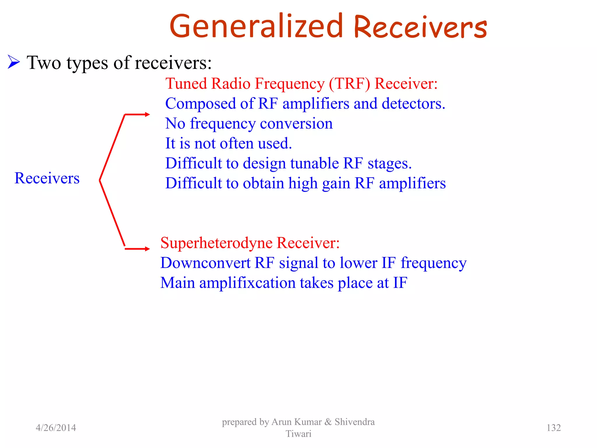


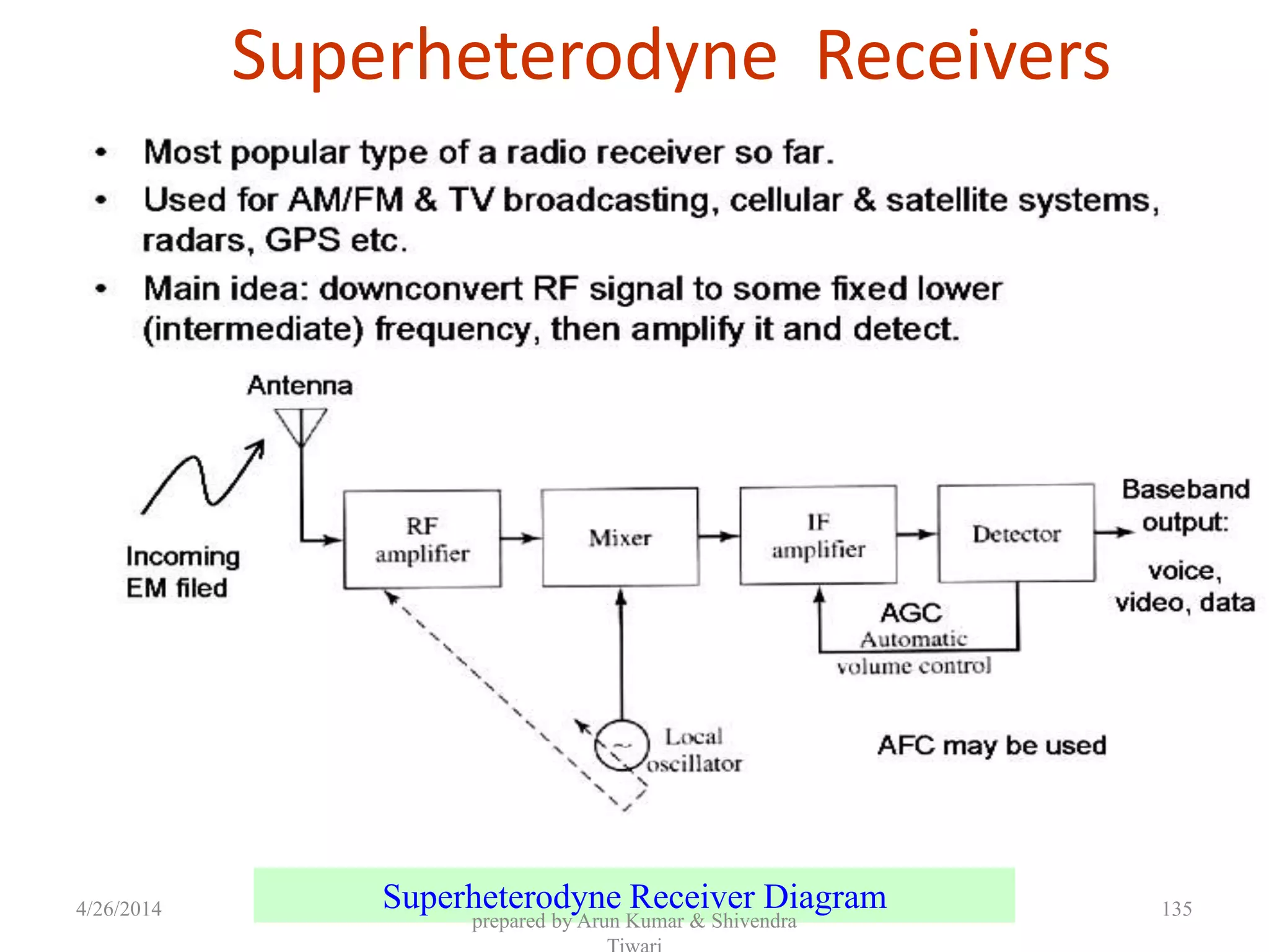
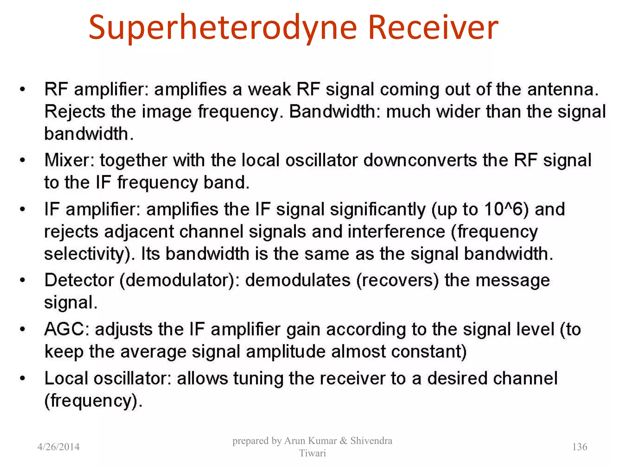
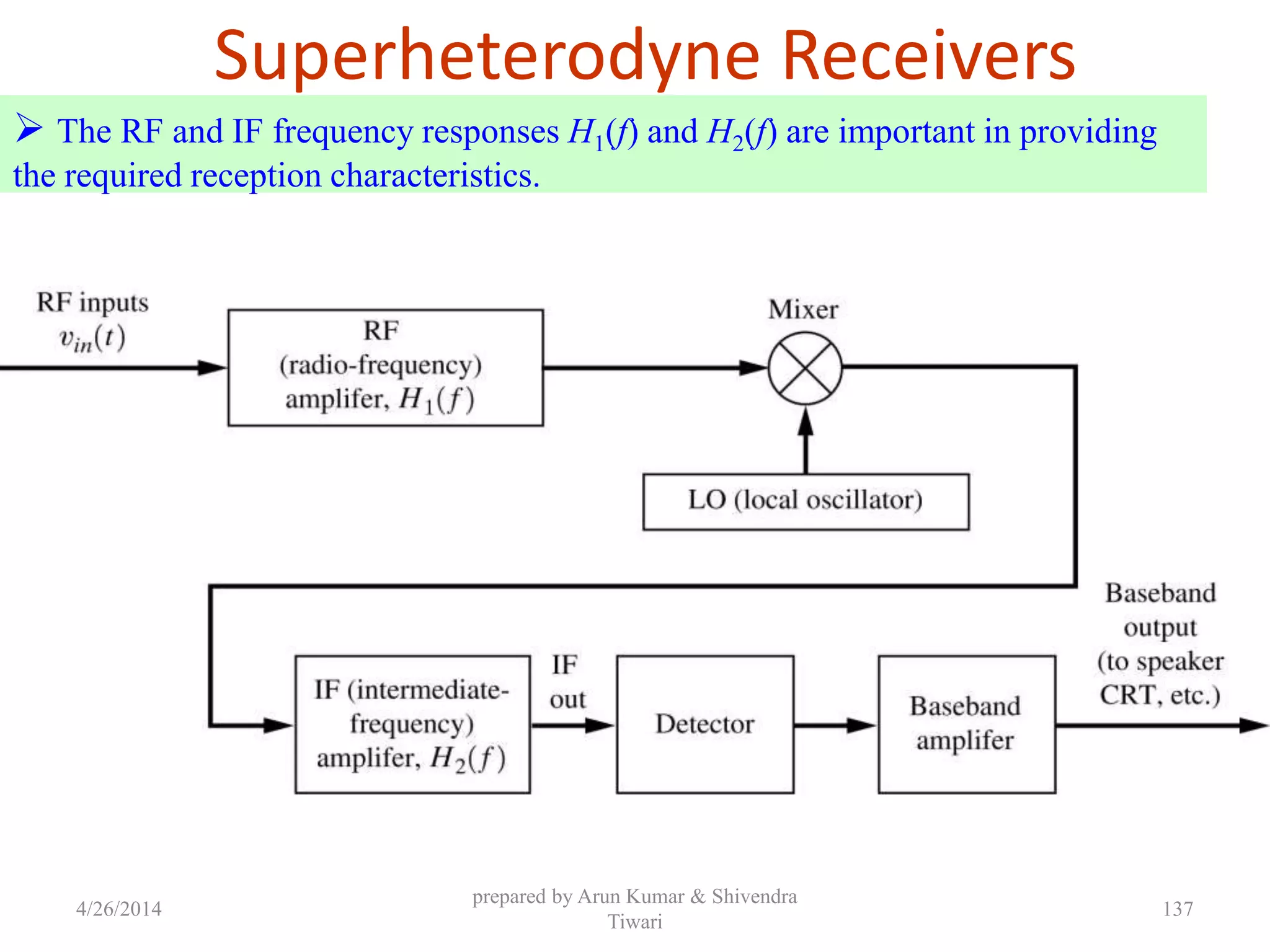


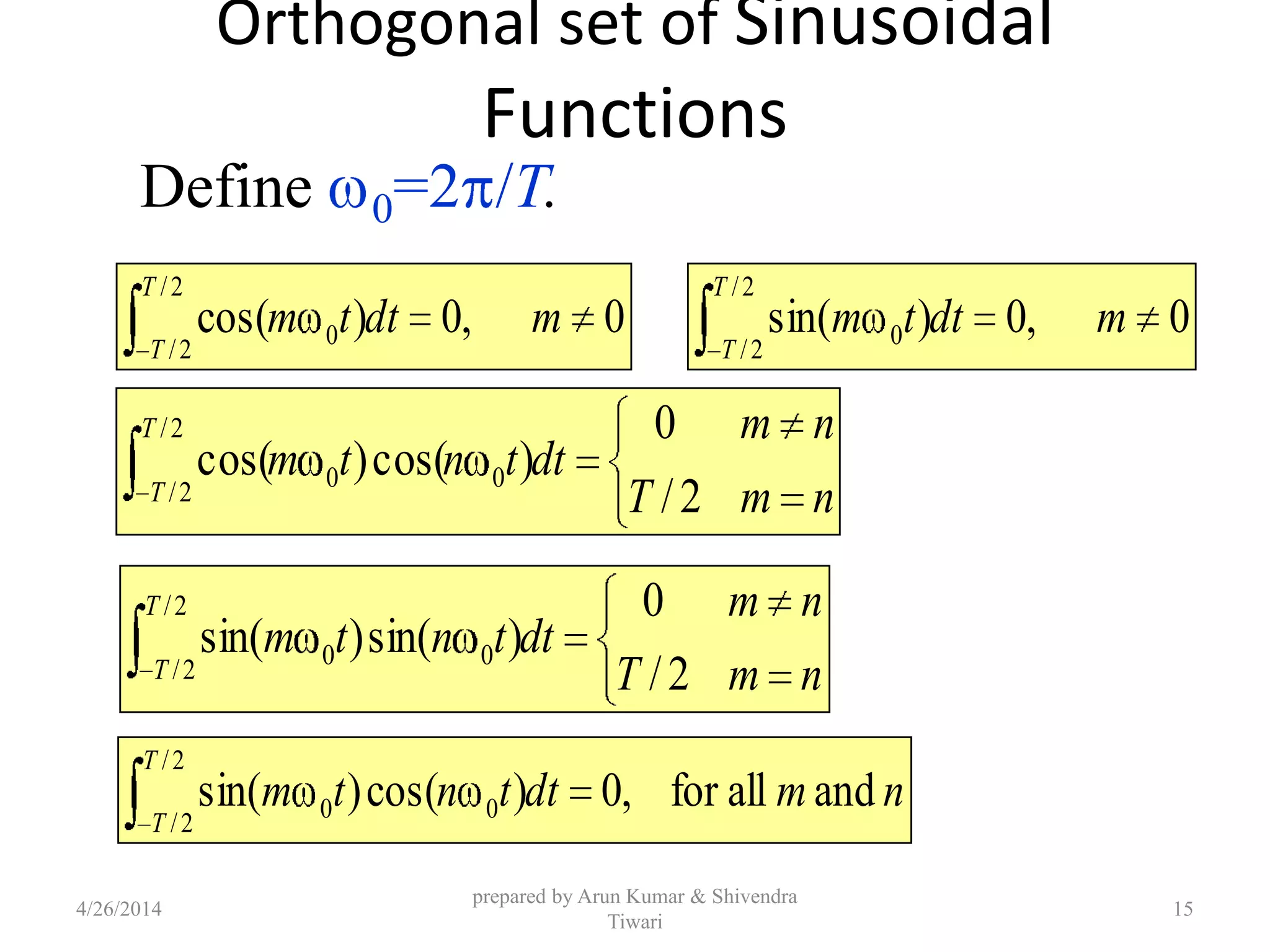
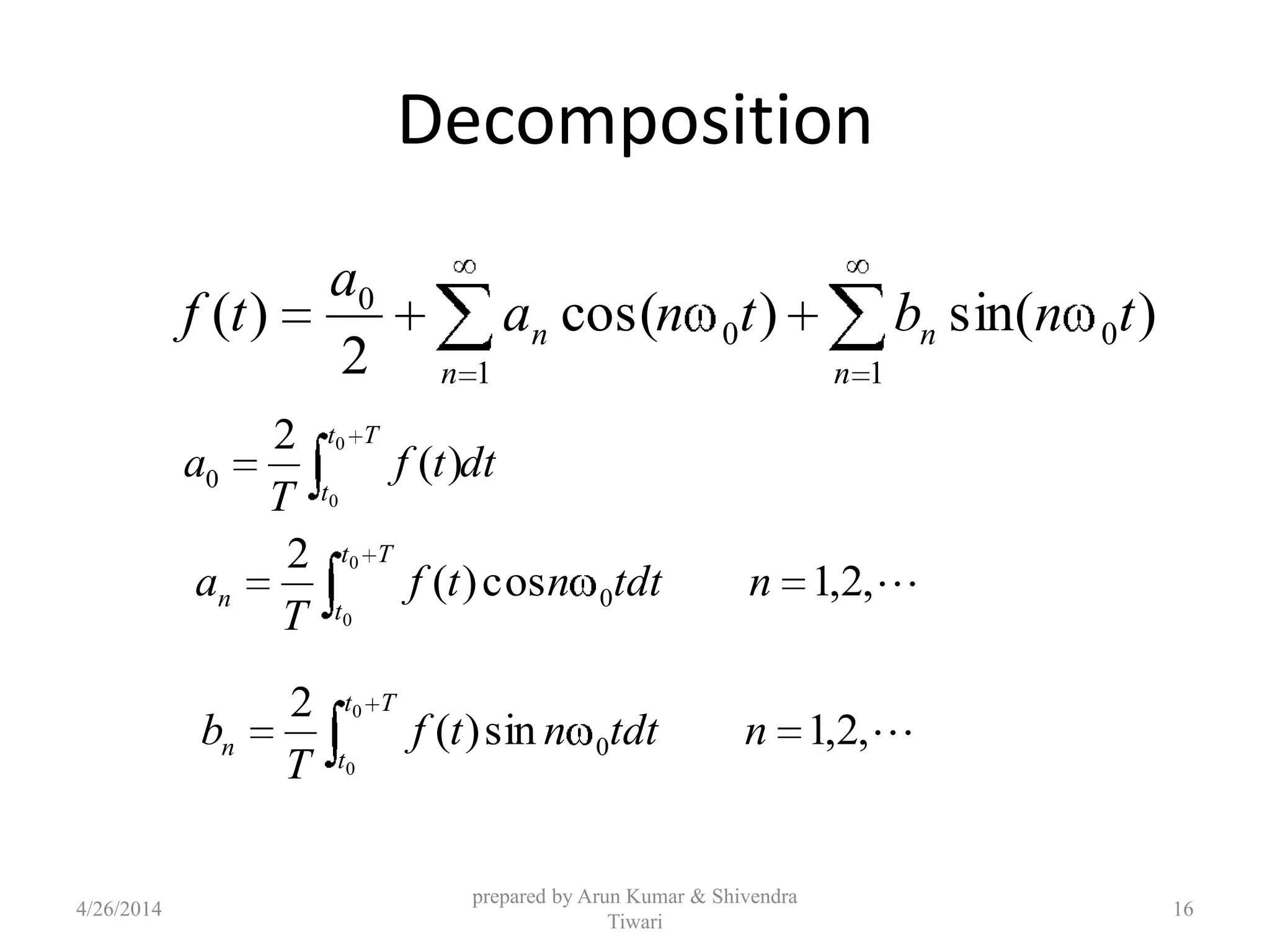
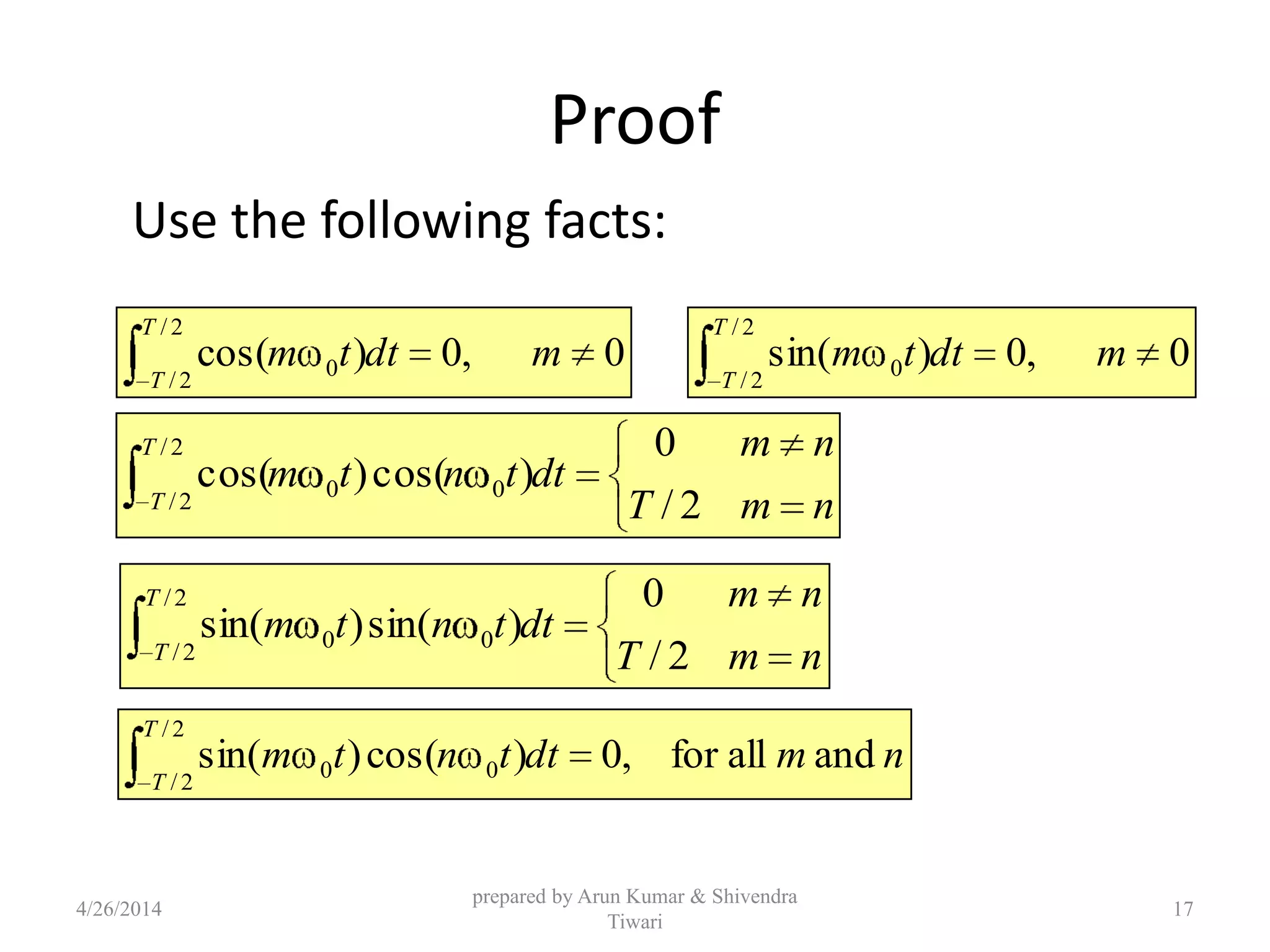
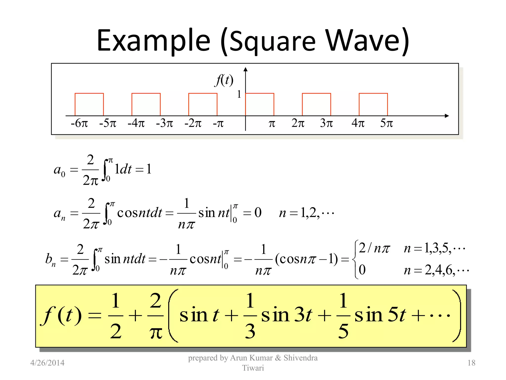
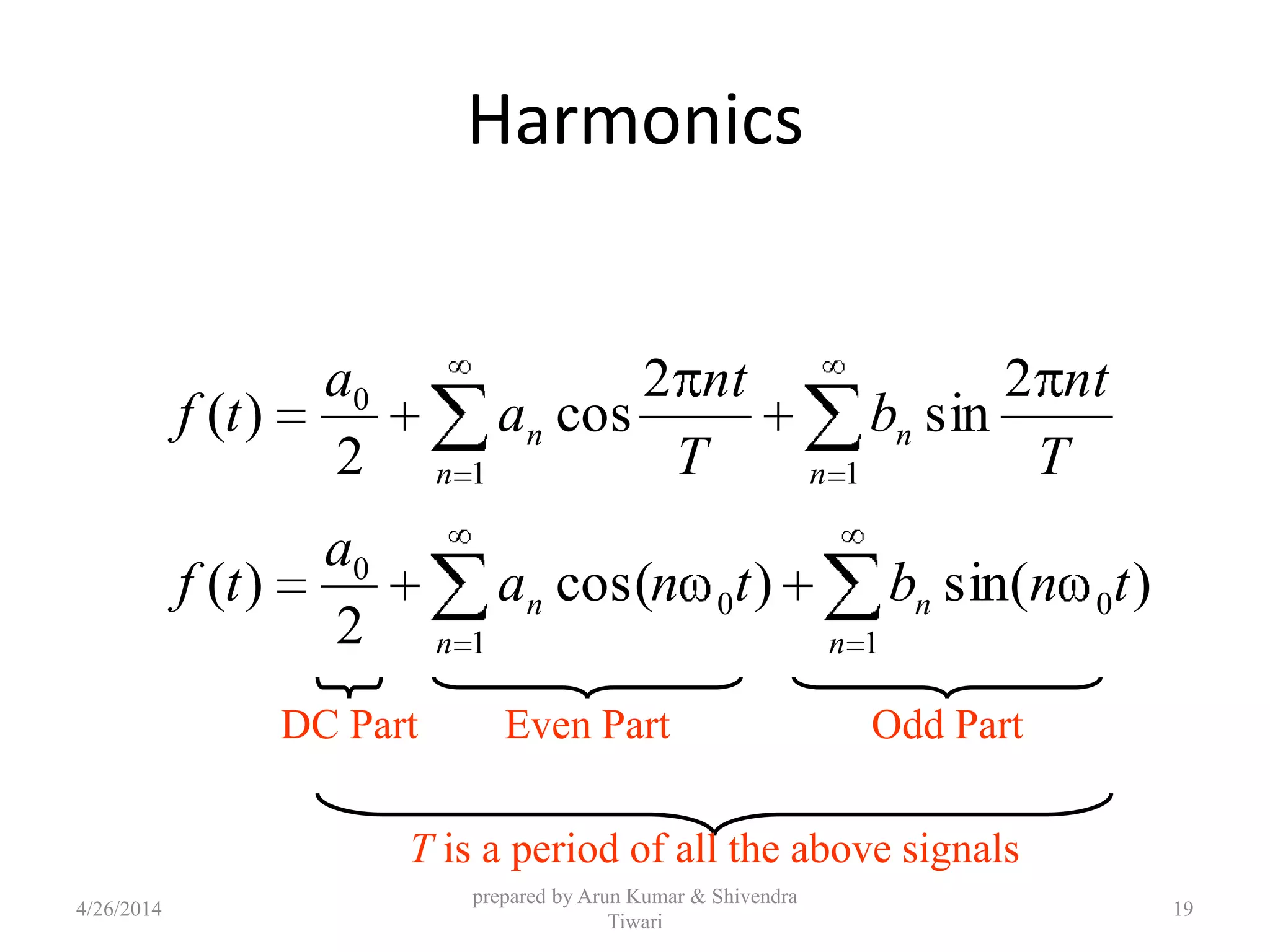
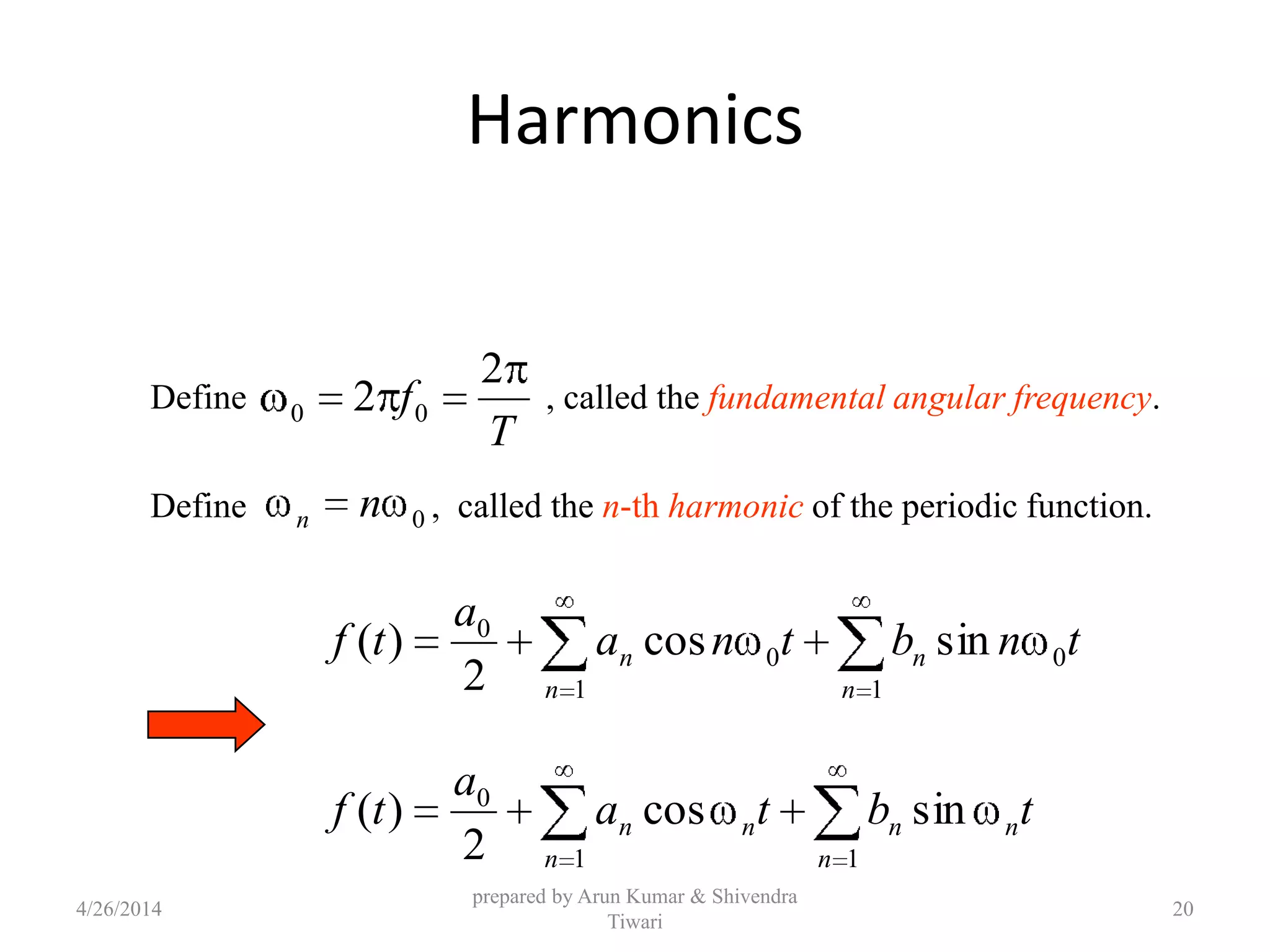
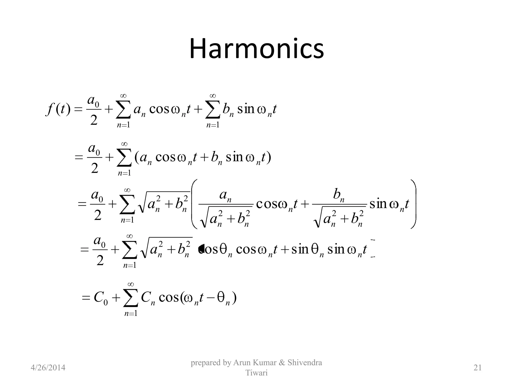
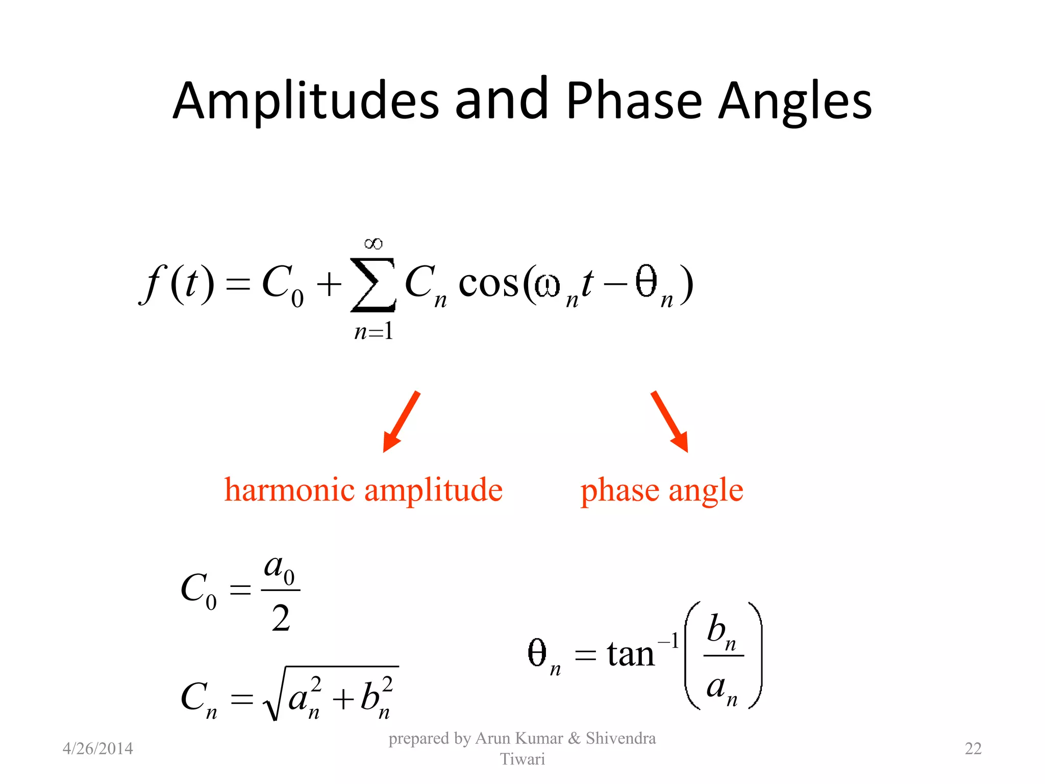
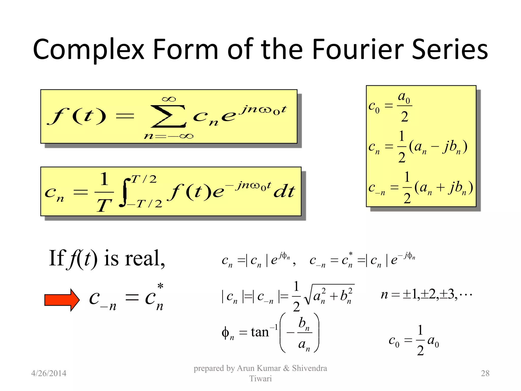
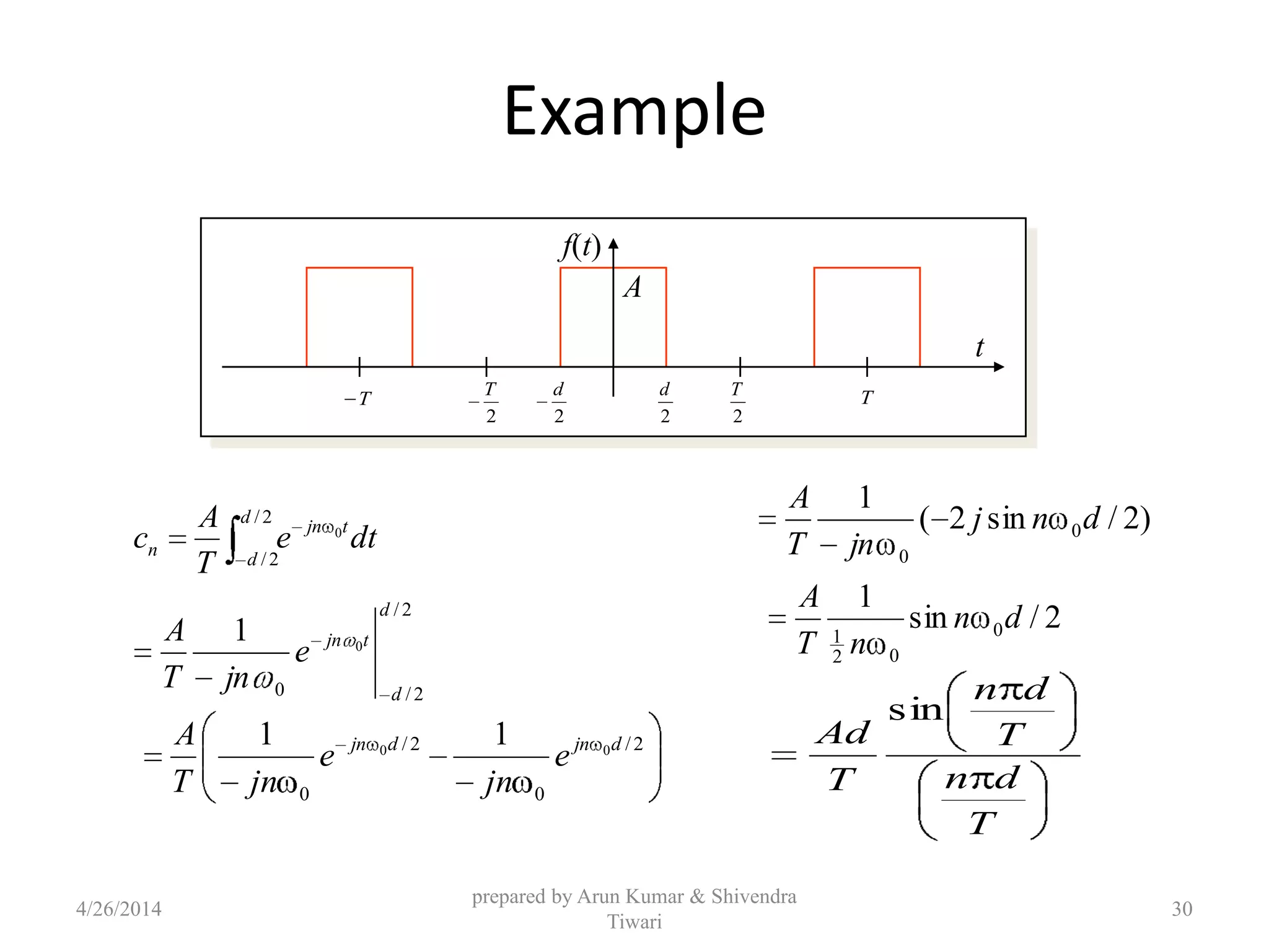
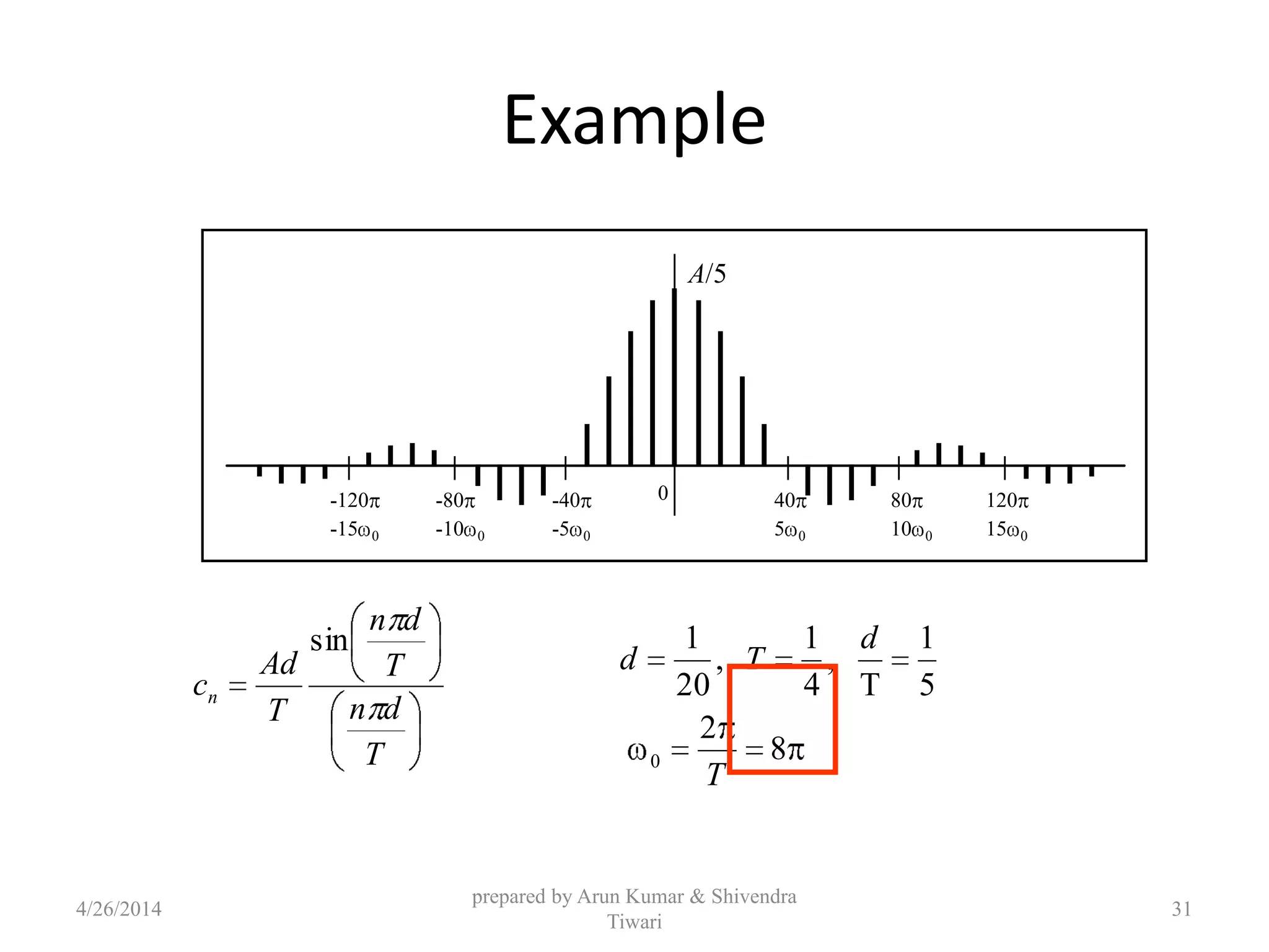
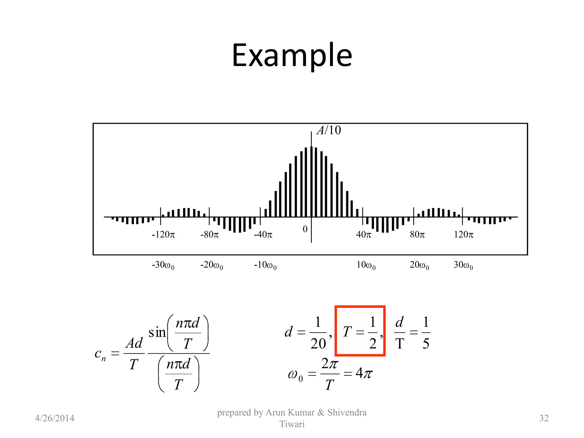
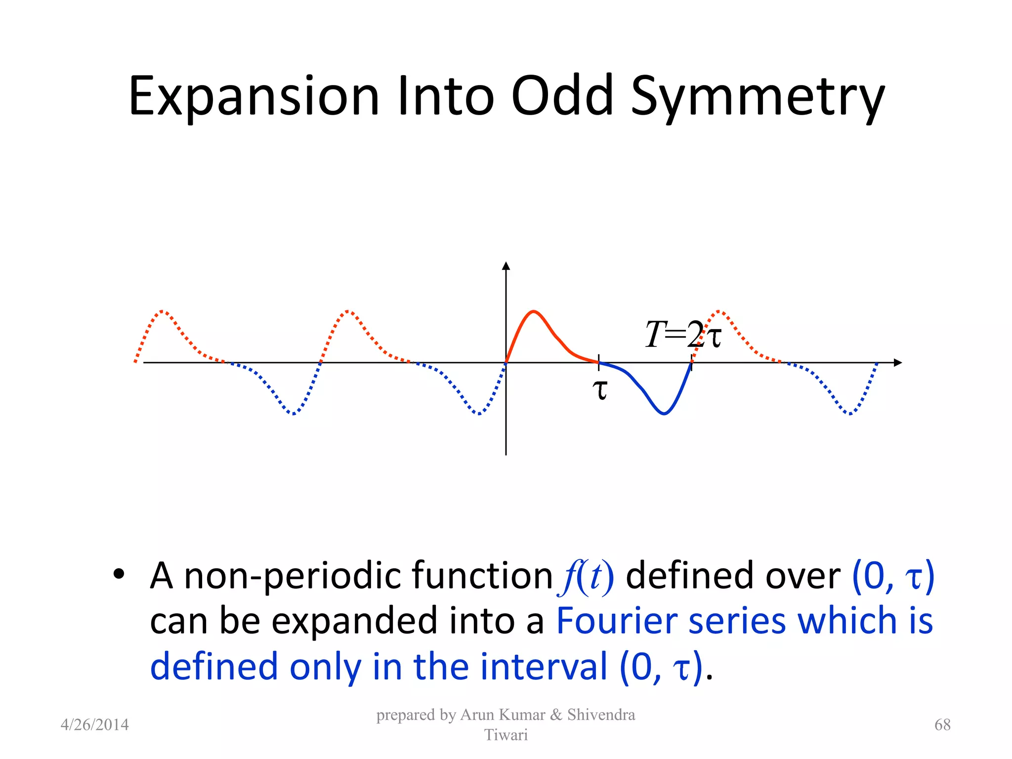
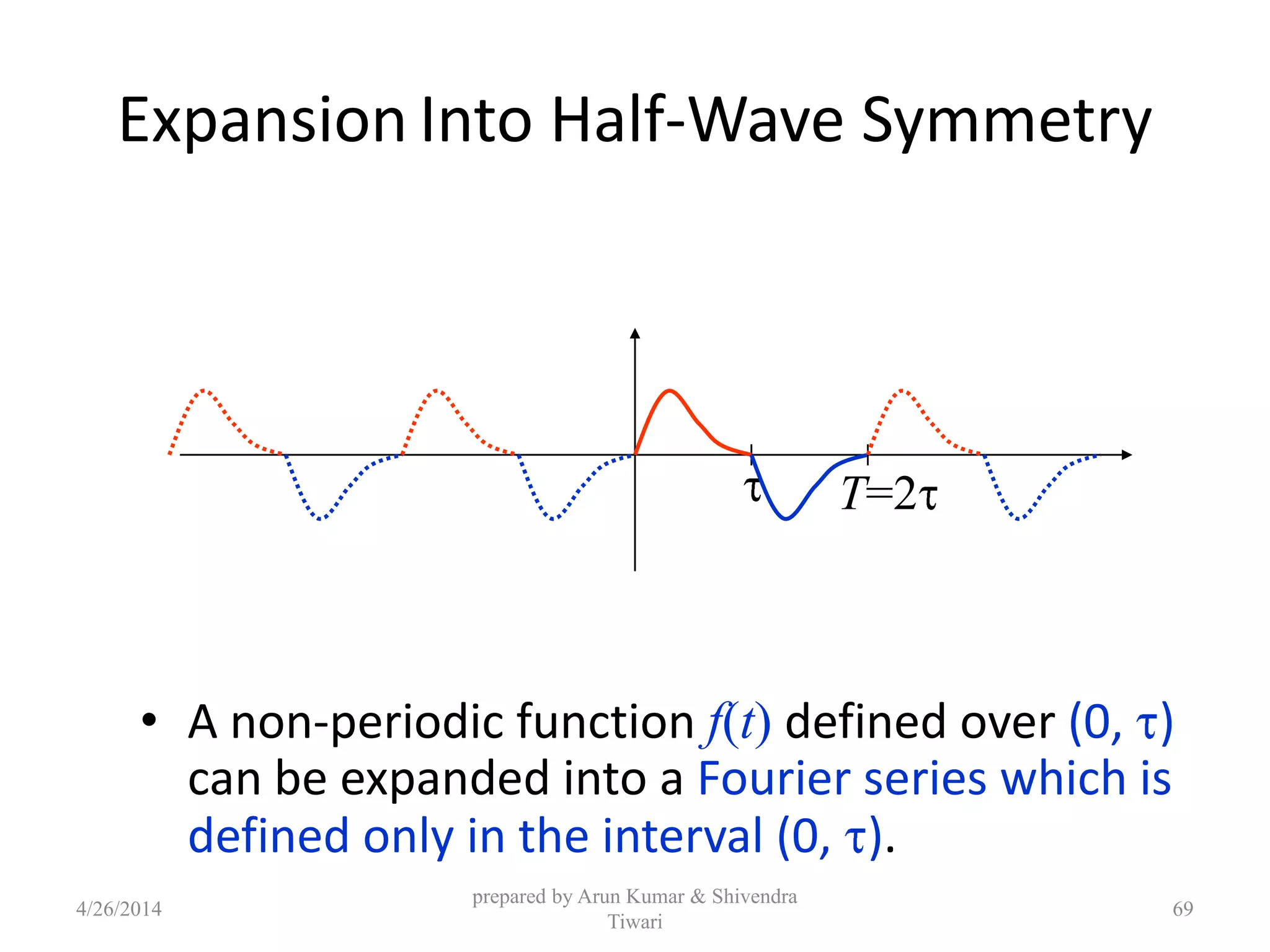
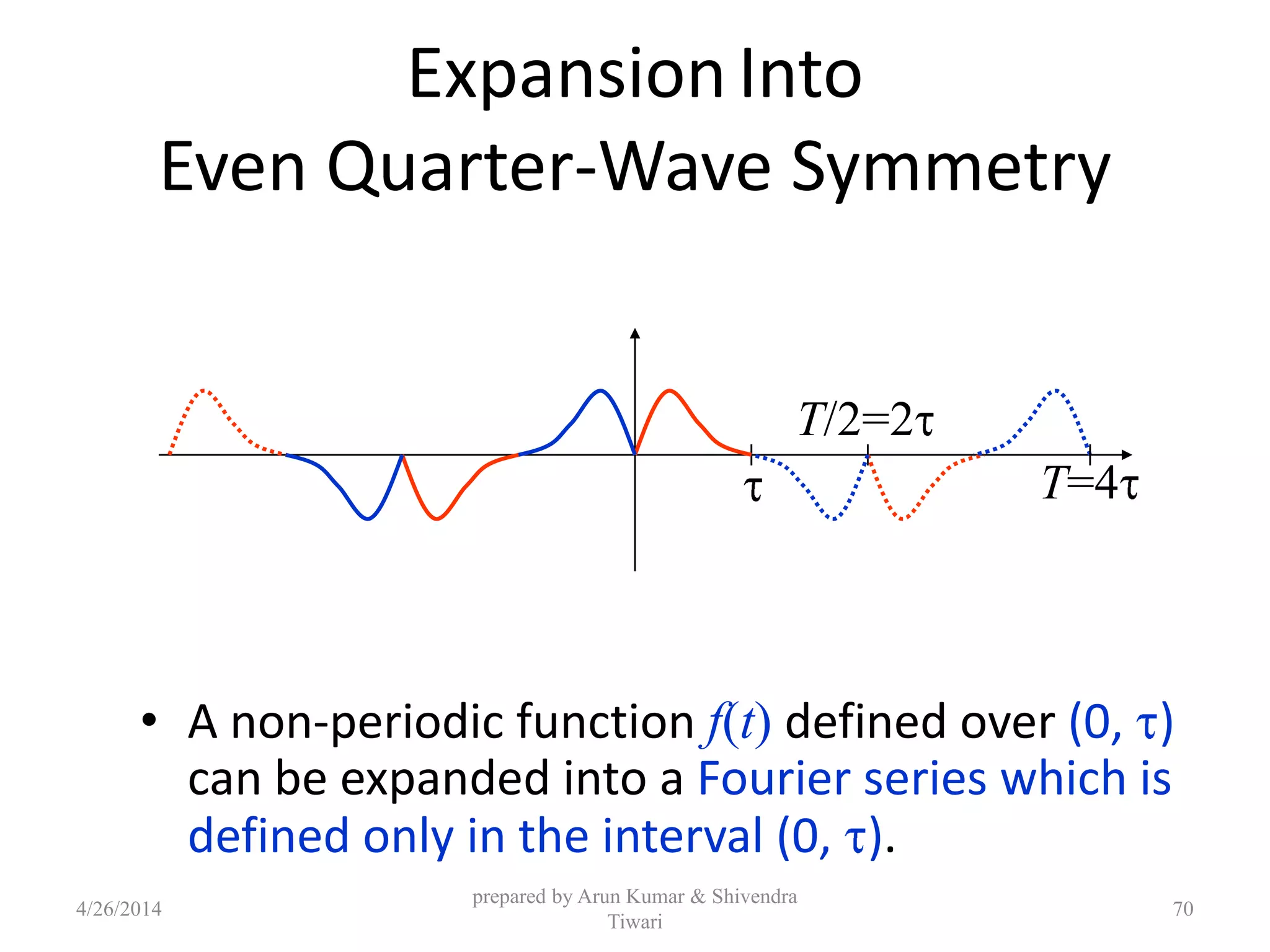
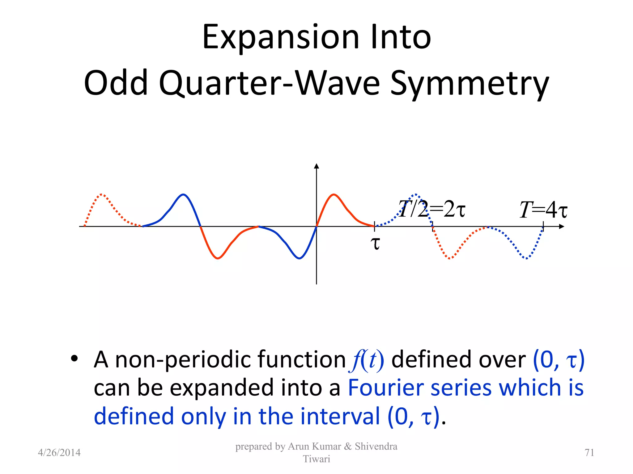
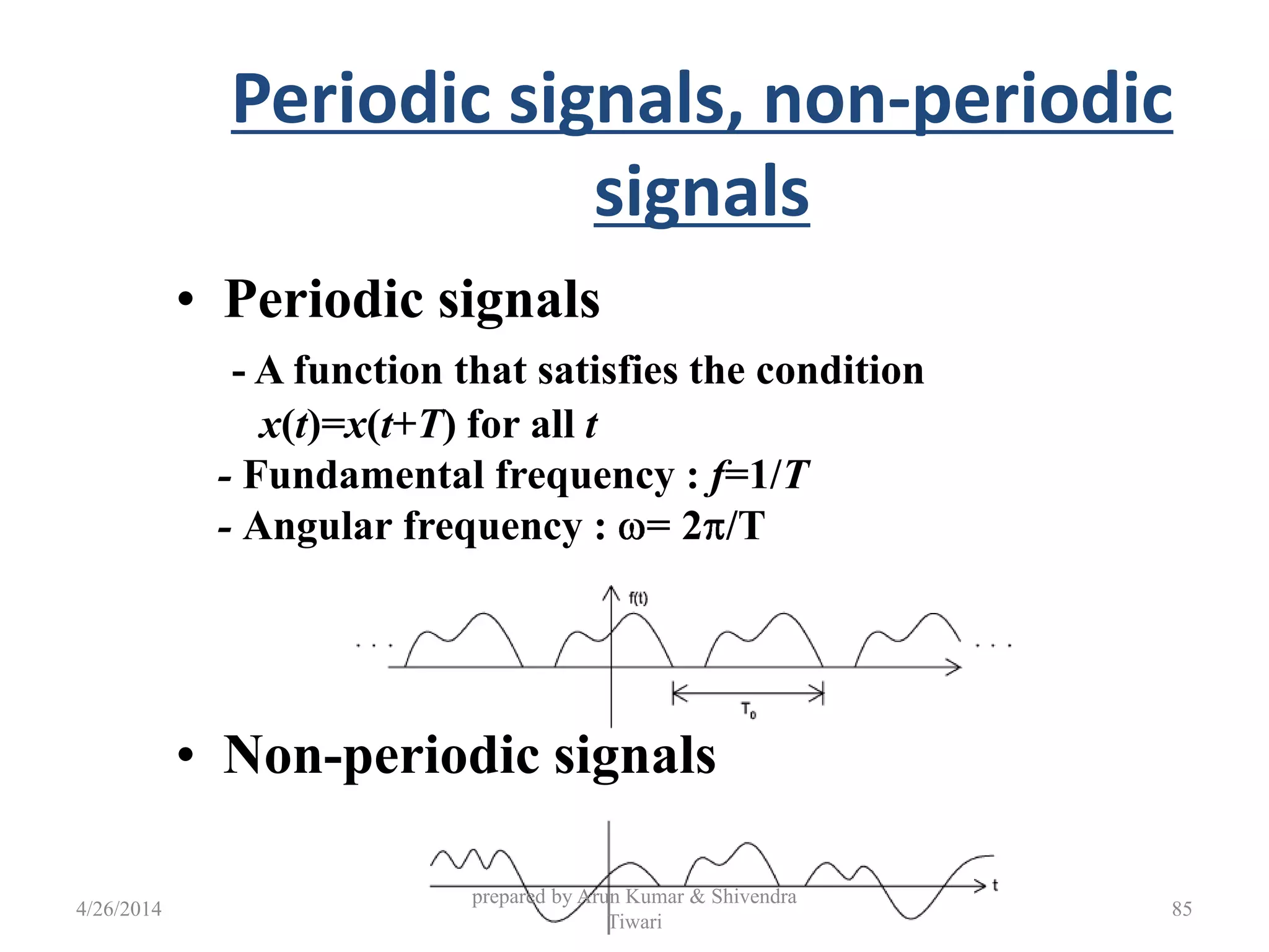
This document provides a summary of signal analysis and Fourier series. It begins by defining periodic functions and using examples to determine the period of periodic signals. It then introduces Fourier series and decomposes periodic signals into a sum of sines and cosines. It describes how these sine and cosine functions form an orthogonal basis and can be used to represent any periodic signal. The document also presents the Fourier series in complex exponential form and uses an example of a square wave to illustrate the decomposition. It defines harmonics and discusses how to determine the amplitude and phase of each harmonic component from the Fourier series coefficients.


![Circuit Network Analysis - [Chapter3] Fourier Analysis](https://cdn.slidesharecdn.com/ss_thumbnails/ch3-150613063858-lva1-app6891-thumbnail.jpg?width=640&height=640&fit=bounds)