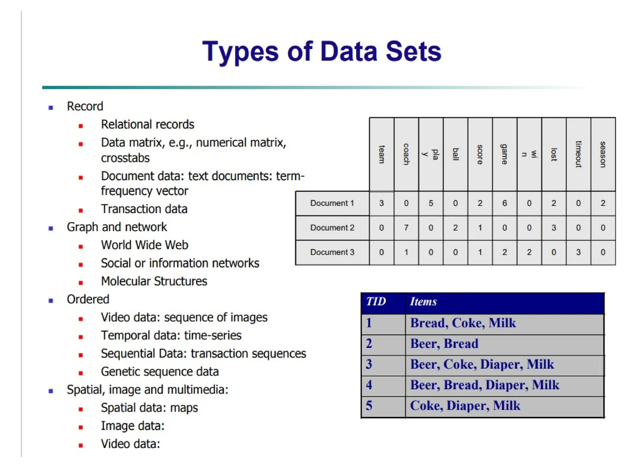
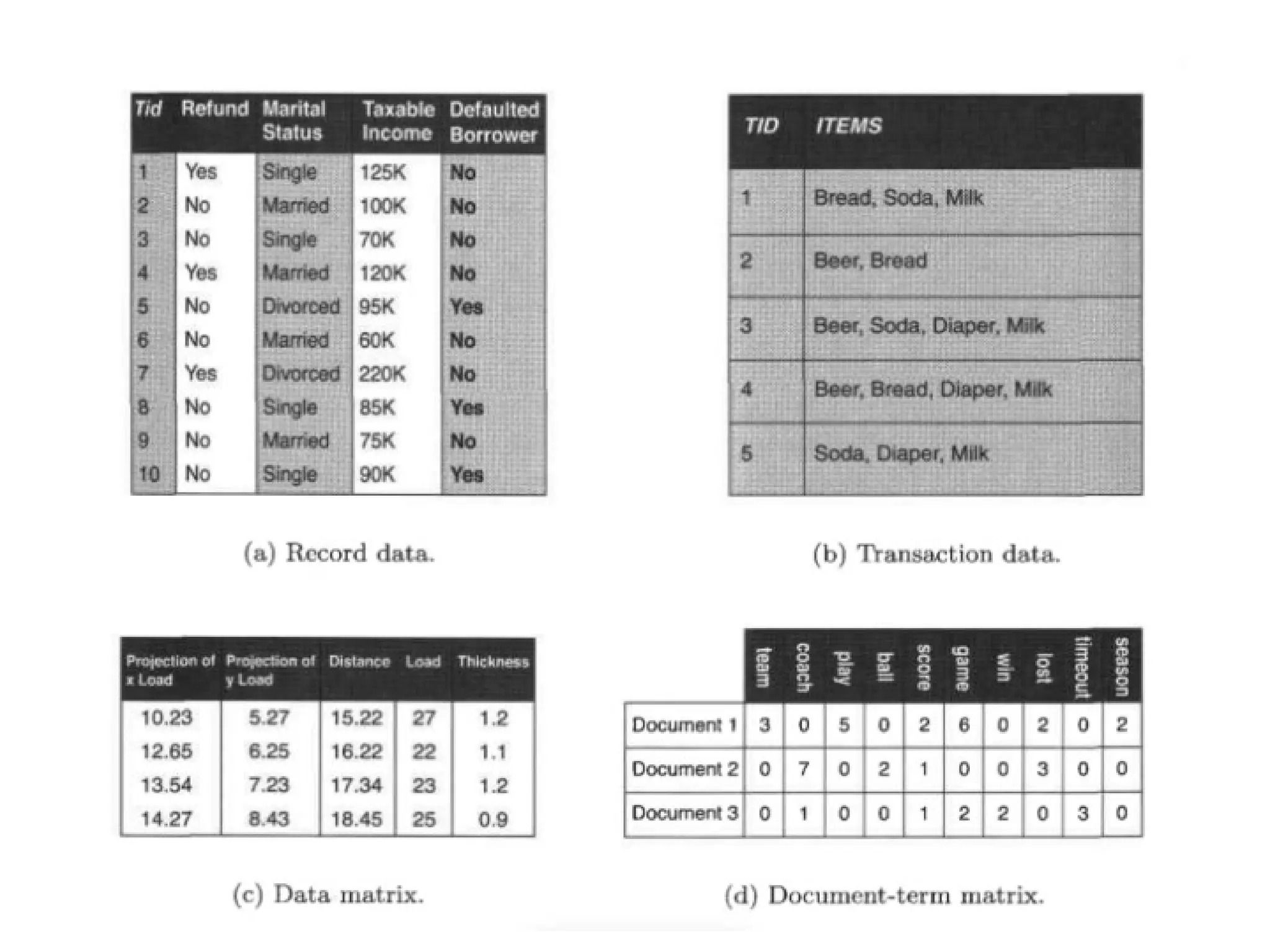
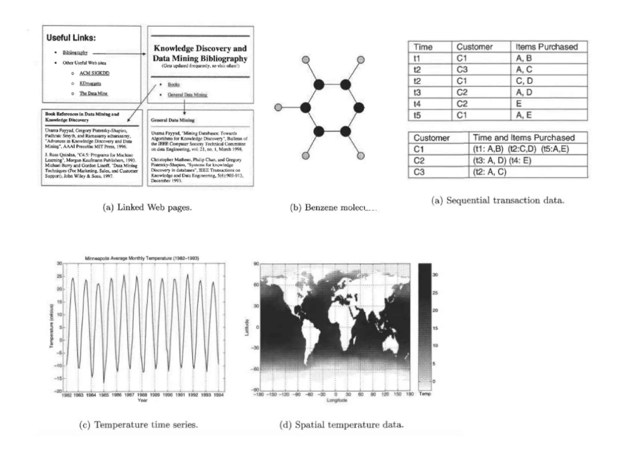
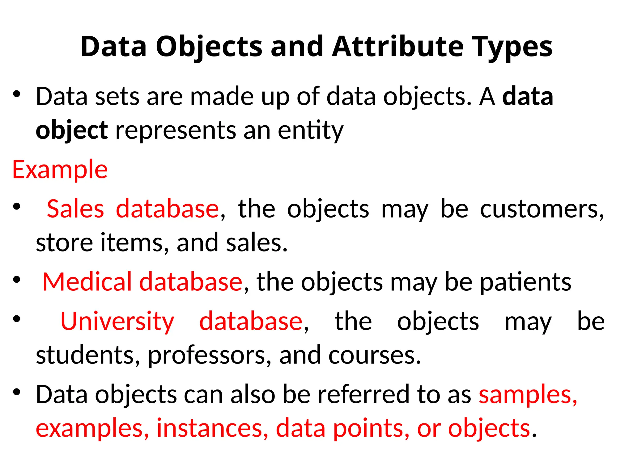
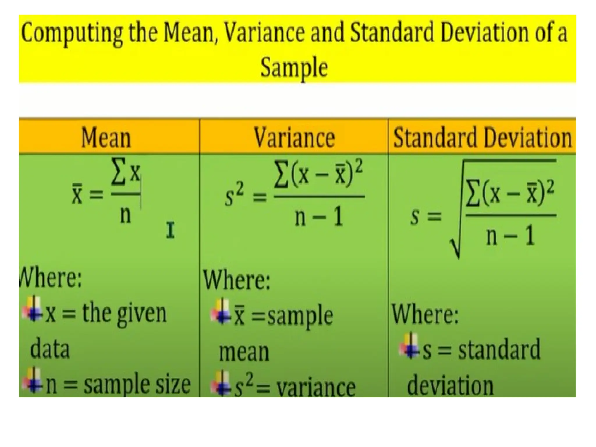
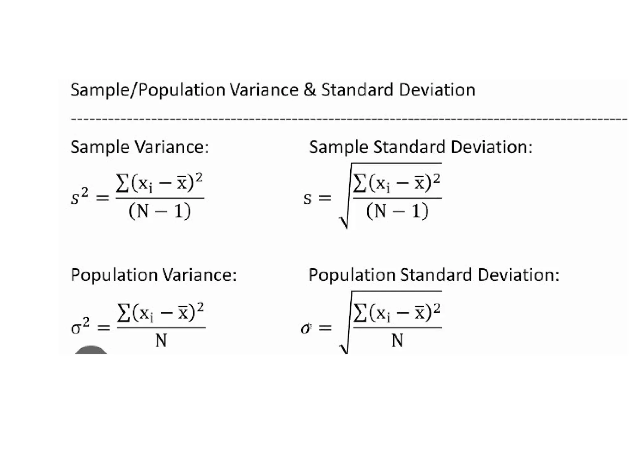
The document provides an overview of basic statistical concepts, including data collection, analysis, and interpretation, emphasizing the role of statistics in data mining and modeling. It explains various concepts such as datasets, data objects, attributes, measures of central tendency (mean, median, mode), and dispersion (variance and standard deviation). Additionally, it discusses skewness, quartiles, interquartile range, and their significance in understanding data distributions.

1. CS3352 & Foundations of Data Science
Basic Statistical Descriptions of Data.
Dr.M.Swarna Sudha
Associate Professor/CSE
Ramco Institute of Technology
Rajapalayam

2. Statistics
• Statistics studies the collection, analysis,
interpretation or explanation, and
presentation of data.
• Data mining has an inherent connection
with statistics.
• A statistical model is a set of
mathematical functions that describe the
behavior of the objects in a target class in
terms of random variables and their
associated probability distributions.

3. • Statistics is useful for mining various patterns
from data as well as for understanding the
underlying mechanisms generating and affecting
the patterns.
• Inferential statistics (or predictive statistics)
models data in a way that accounts for
randomness and uncertainty in the observations
and is used to draw inferences about the process
or population under investigation

4. Dataset
• A dataset in machine learning is, quite
simply, a collection of data pieces that can be
treated by a computer as a single unit for
analytic and prediction purposes

8. Data Objects and Attribute Types
• Data sets are made up of data objects. A data
object represents an entity
Example
• Sales database, the objects may be customers,
store items, and sales.
• Medical database, the objects may be patients
• University database, the objects may be
students, professors, and courses.
• Data objects can also be referred to as samples,
examples, instances, data points, or objects.

9. What Is an Attribute?
• An attribute is a data field, representing a
characteristic or feature of a data object.
• Attribute, dimension, feature, and variable are
often used
• The term dimension is commonly used in data
warehousing.
• Machine learning use the term feature, while
statisticians prefer the term variable.

12. Attribute Types

13. Numeric Attribute Type

16. Measuring the Central Tendency: Mean,
Median, and Mode
• Suppose that we have some attribute X, like salary,
which has been recorded for a set of objects. Let
x1,x2,...,xN be the set of N observed values or
observations for X.
• Here, these values may also be referred to as the data
set (for X).
• If we were to plot the observations for salary, where
would most of the values fall? This gives us an idea of
the central tendency of the data.
• Measures of central tendency include the mean,
median, mode, and midrange.

17. • The most common and effective numeric
measure of the “center” of a set of data is the
(arithmetic) mean.
• Let x1,x2,...,xN be a set of N values or
observations, such as for some numeric
attribute X, like salary.
• The mean of this set of values is

18. Examples
• Mean. Suppose we have the following values
for salary (in thousands of dollars), shown in
increasing order: 30, 36, 47, 50, 52, 52, 56, 60,
63, 70, 70, 110.

20. •
Trimmed mean
• Even a small number of extreme values can corrupt
the mean.
• For example, the mean salary at a company may be
substantially pushed up by that of a few highly paid
managers.
• Similarly, the mean score of a class in an exam could
be pulled down quite a bit by a few very low scores.
• To offset the effect caused by a small number of
extreme values, we can instead use the trimmed
mean

21. • Median. Suppose we have the following values for
salary (in thousands of dollars), shown in increasing
order: 30, 36, 47, 50, 52, 52, 56, 60, 63, 70, 70, 110)
• The data are already sorted in increasing order. There
is an even number of observations (i.e., 12);
• therefore, the median is not unique.
• It can be any value within the two middlemost
values of 52 and 56 (that is, within the sixth and
seventh values in the list).
• By convention, we assign the average of the two
middlemost values as the median; that is,
• (52+56 )/2 = 108 /2 = 54.
Thus, the median is $54,000

22. • Suppose that we had only the first 11 values in
the list. Given an odd number of values, the
median is the middlemost value. This is the
sixth value in this list, which has a value of
$52,000.
• The median is expensive to compute when we
have a large number of observations.

23. where L1 is the lower boundary of the median interval,
n is the number of values in the entire data set,
Freqmedian is the frequency of the median interval, and width is the width of
the median interval.
is the sum of the frequencies of all of the intervals

24. • Mode : Suppose we have the following values for
salary (in thousands of dollars), shown in increasing
order: 30, 36, 47, 50, 52, 52, 56, 60, 63, 70, 70, 110)
• The two modes are $52,000 and $70,000.
• The mode for a set of data is the value that occurs
most frequently in the set.
• Therefore, it can be determined for qualitative
and quantitative attributes
• Data sets with one, two, or three modes are
respectively called unimodal, bimodal, and
trimodal. In general, a data set with two or more
modes is multimodal.

25. • For unimodal numeric data that are moderately
skewed (asymmetrical),
• we have the following empirical relation: mean −
mode ≈ 3 × (mean − median).
• This implies that the mode for unimodal frequency
curves that are moderately skewed can easily be
approximated if the mean and median values are
known.
• The midrange can also be used to assess the central
tendency of a numeric data set.
• It is the average of the largest and smallest values in
the set

26. • Suppose we have the following values for salary (in
thousands of dollars), shown in increasing order: 30, 36, 47,
50, 52, 52, 56, 60, 63, 70, 70, 110)
• Midrange. The midrange of the data of Example 2.6 is
30,000+110,000 2 = $70,000.
• In a unimodal frequency curve with perfect symmetric
data distribution, the mean, median, and mode are all at
the same center value, as shown in Figure 2.1(a).
• Data in most real applications are not symmetric. They
may instead be either positively skewed, where the mode
occurs at a value that is smaller than the median (Figure
2.1b),
• or negatively skewed, where the mode occurs at a value
greater than the median (Figure 2.1c).

29. Skewness
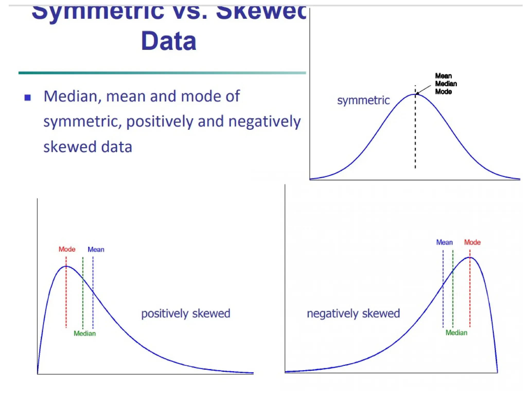
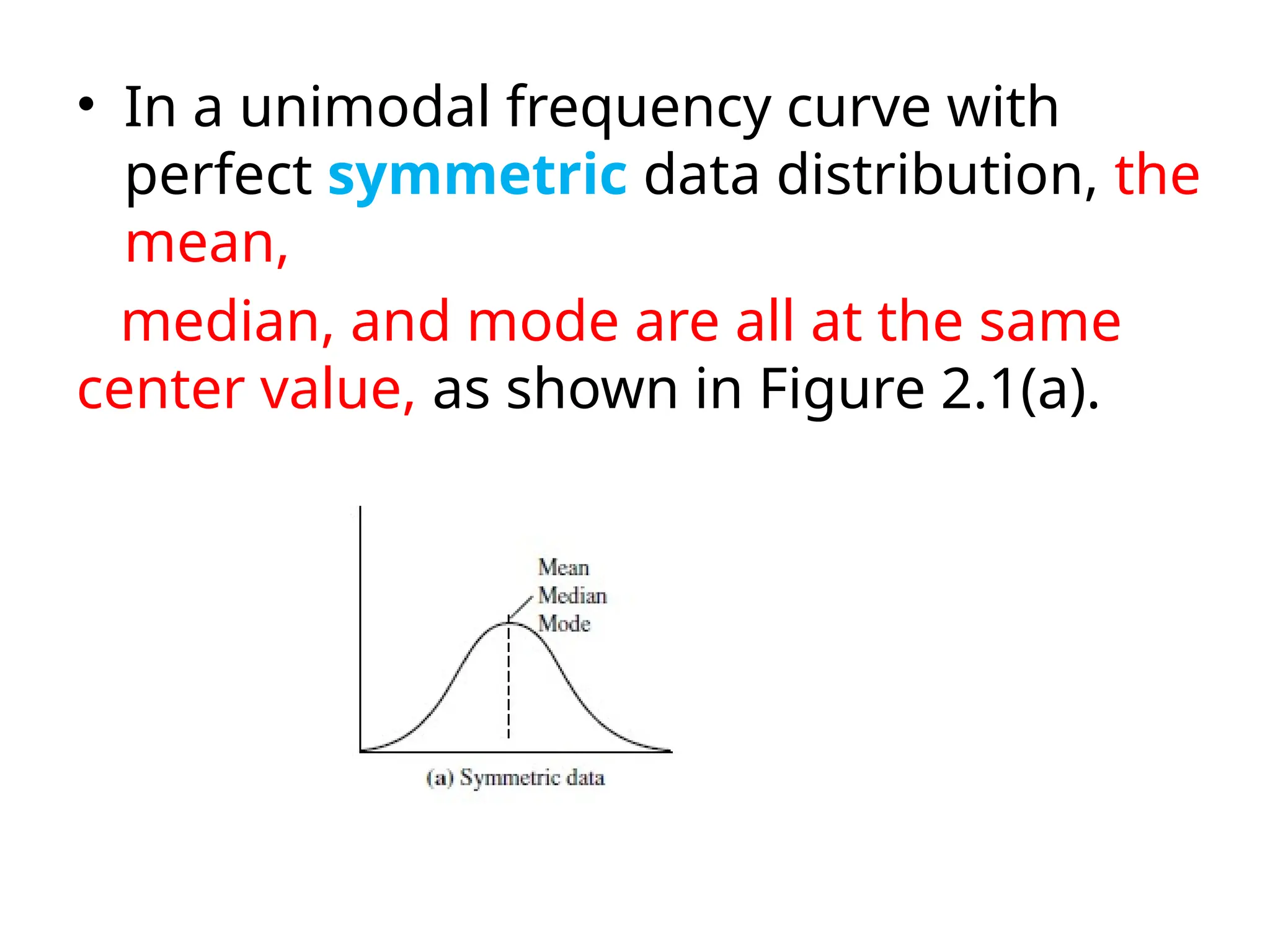
• Skewness is used to measure symmetry of data
along with the mean value. Symmetry means equal
distribution of observation above or below the mean.
• skewness = 0: if data is symmetric along with mean
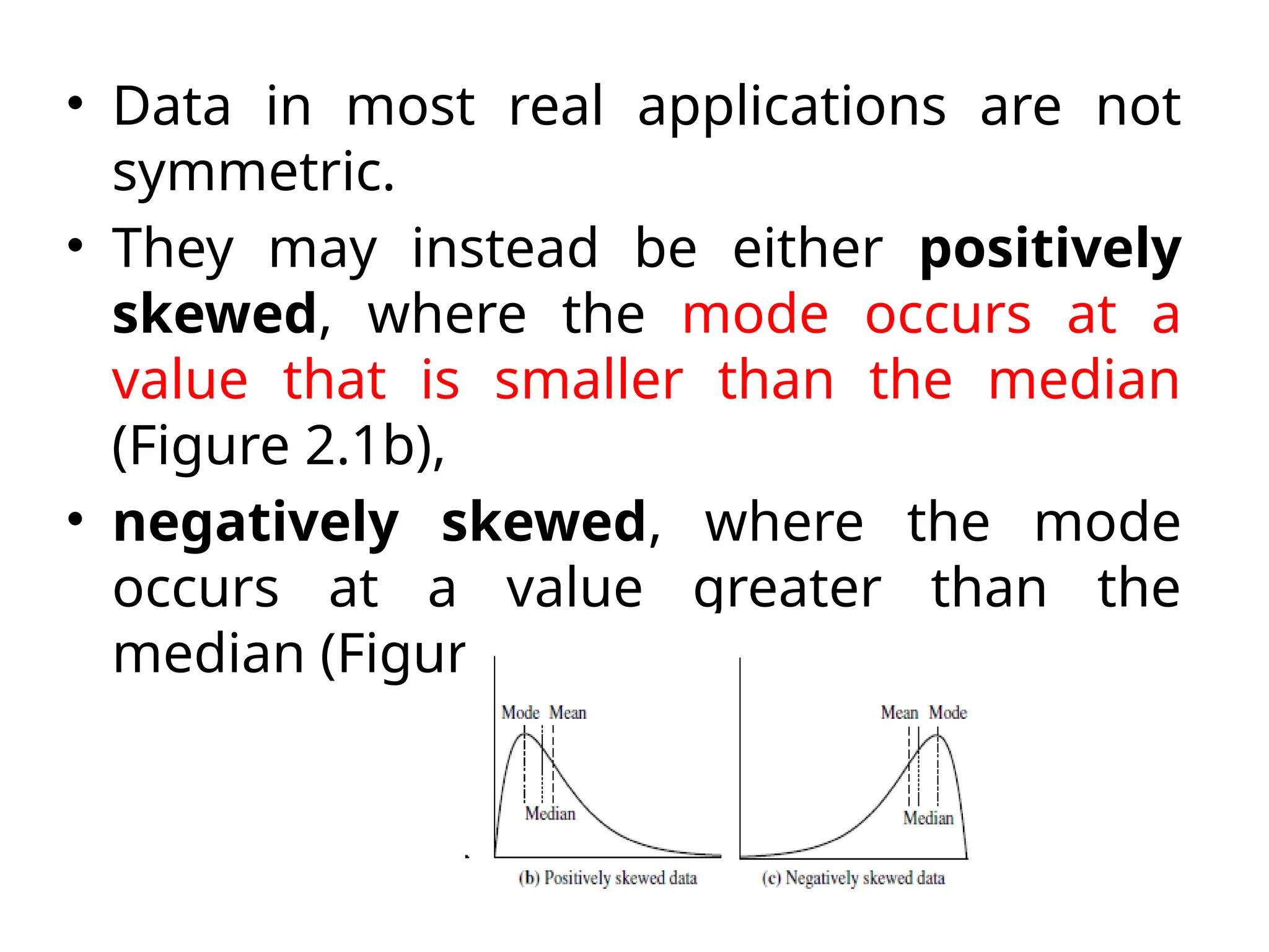
• skewness = Negative: if data is not symmetric and
right side tail is longer than left side tail of density
plot.
• skewness = Positive: if data is not symmetric and
left side tail is longer than right side tail in density
plot.
• We can find skewness of given variable by below
given formula.
• data[‘A’].skew()

30. • In a unimodal frequency curve with
perfect symmetric data distribution, the
mean,
median, and mode are all at the same
center value, as shown in Figure 2.1(a).

31. • Data in most real applications are not
symmetric.
• They may instead be either positively
skewed, where the mode occurs at a
value that is smaller than the median
(Figure 2.1b),
• negatively skewed, where the mode
occurs at a value greater than the
median (Figure 2.1c).

32. Range, Quartiles, and
Interquartile Range

34. Range, Quartiles, and Interquartile Range
• Let x1,x2,...,xN be a set of observations for
some numeric attribute, X.
• The range of the set is the difference between
the largest (max()) and smallest (min()) values

37. • Suppose that the data for attribute X are
sorted in increasing numeric order. Imagine
that we can pick certain data points so as to
split the data distribution into equal-size
consecutive sets, as in Figure

48. Examples
• 75, 69, 56, 46, 47, 79, 92, 97, 89, 88, 36, 96, 105, 32, 116, 101, 79, 93,
91, 112
• After sorting the above data set:
32, 36, 46, 47, 56, 69, 75, 79, 79, 88, 89, 91, 92, 93, 96, 97, 101, 105,
112, 116
• Here the total number of terms is 20.
• The second quartile (Q2) or the median of the above data is (88 +
89) / 2 = 88.5
• The first quartile (Q1) is median of first n i.e. 10 terms (or n i.e. 10
smallest values) = 62.5
• The third quartile (Q3) is the median of n i.e. 10 largest values (or last
n i.e. 10 values) = 96.5
• Then, IQR = Q3 – Q1 = 96.5 – 62.5 = 34.0

50. • The IQR is used to build box plots, simple graphical
representations of a probability distribution.
• The IQR can also be used to identify the outliers in the given
data set.
• The IQR gives the central tendency of the data.
Decision Making
• The data set has a higher value of interquartile range (IQR)
has more variability.
• The data set having a lower value of interquartile range
(IQR) is preferable.
• Suppose if we have two data sets and their interquartile
ranges are IR1 and IR2, and if IR1 > IR2 then the data in IR1
is said to have more variability than the data in IR2 and data
in IR2 is preferable.
USE of IQR

51. Variance and Standard Deviation
• Variance and standard deviation are measures
of data dispersion.
• They indicate how spread out a data
distribution is.
• A low standard deviation means that the data
observations tend to be very close to the
mean, while a high standard deviation
indicates that the data are spread out over a
large range of values.