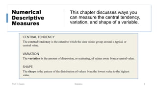
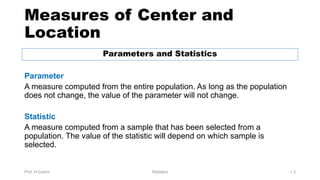
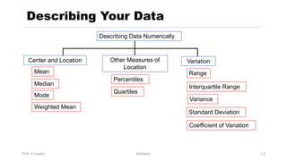
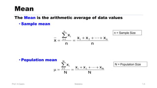
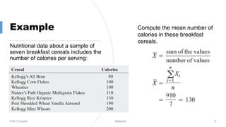
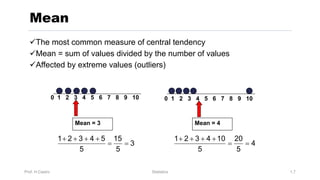
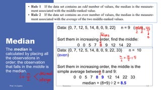
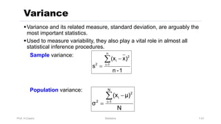
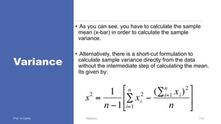
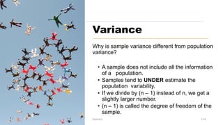
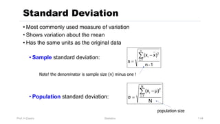
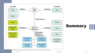
Stats - Lecture CH 3- Describing Data Using Numerical Measures.pdf

Chapter 3:
Describing
Data Using
Numerical
Measures
Prof. Hilmar Castro
QLU - Panmá
Prof. H.Castro Statistics 1

This chapter discusses ways you
can measure the central tendency,
variation, and shape of a variable.
Numerical
Descriptive
Measures

Measures of Center and
Location
Parameters and Statistics
Parameter
A measure computed from the entire population. As long as the population
does not change, the value of the parameter will not change.
Statistic
A measure computed from a sample that has been selected from a
population. The value of the statistic will depend on which sample is
selected.
Prof. H.Castro Statistics 1.3

Describing Your Data
Center and Location
Mean
Median
Mode
Other Measures of
Location
Weighted Mean
Describing Data Numerically
Variation
Variance
Standard Deviation
Coefficient of Variation
Range
Percentiles
Interquartile Range
Quartiles

Mean
N
x
x
x
N
x
N
N
i
i
+
+
+
=
=
µ
å
= !
2
1
1
n
x
x
x
n
x
x n
n
i
i
+
+
+
=
=
å
= !
2
1
1
The Mean is the arithmetic average of data values
• Sample mean
• Population mean
n = Sample Size
N = Population Size

Example
Nutritional data about a sample of
seven breakfast cereals includes the
number of calories per serving:
Compute the mean number of
calories in these breakfast
cereals.

Mean
üThe most common measure of central tendency
üMean = sum of values divided by the number of values
üAffected by extreme values (outliers)
0 1 2 3 4 5 6 7 8 9 10
Mean = 3 Mean = 4
3
5
15
5
5
4
3
2
1
=
=
+
+
+
+
4
5
20
5
10
4
3
2
1
=
=
+
+
+
+
0 1 2 3 4 5 6 7 8 9 10

Median
The median is
calculated by placing all
the observations in
order; the observation
that falls in the middle is
the median.
Statistics 1.8
Data: {0, 7, 12, 5, 14, 8, 0, 9, 22} n = 9 (odd)
Sort them in increasing order, find the middle:
0 0 5 7 8 9 12 14 22
Data: {0, 7, 12, 5, 14, 8, 0, 9, 22, 33} n = 10
(even)
Sort them in increasing order, the middle is the
simple average between 8 and 9:
0 0 5 7 8 9 12 14 22 33
median = (8+9)÷2 = 8.5

Median
§Not affected by extreme values
§In an ordered array, the median is the “middle” number
§If n or N is odd, the median is the middle number
§If n or N is even, the median is the average of the two middle numbers
Median = 2 Median = 2

Skewed and Symmetric
Distributions
Skewed Data
Data sets that are not symmetric. For skewed data, the mean will be larger or smaller than
the median.
Symmetric Data
Data sets whose values are evenly spread around the center. For symmetric data, the mean
and median are equal.
Right-Skewed Data
A data distribution is right skewed if the mean for the data is larger than the median.
Left-Skewed Data
A data distribution is left skewed if the mean for the data is smaller than the median.

Mode
• A measure of central tendency
• Value that occurs most often
• Not affected by extreme values
• Used for either numerical or categorical data
• There may be no mode
• There may be several modes
Frequency
Variable
MODAL CLASS
Mode = 5 No Mode
0 1 2 3 4 5 6 7 8 9 10 11 12 13 14 0 1 2 3 4 5 6

Mode
§The mode of a set of observations is the value that occurs most
frequently.
§A set of data may have one mode (or modal class), or two, or more
modes.
§Mode is a useful for all data types, though mainly used for nominal
data.
§For large data sets the modal class is much more relevant than a
single-value mode.
§Sample and population modes are computed the same way.

Mean, Median, Mode
§For ordinal and nominal data the calculation of the mean is NOT valid.
§Median is appropriate for ordinal data.
§For nominal data, a mode calculation is useful for determining highest
frequency but not “central location”.
§If data are symmetric, the mean, median, and mode will be approximately
the same.
§If data are skewed, or have outliers, report the MEDIAN.
§Mean is very sensitive to extreme values called “outliers”.
§If data are multimodal, report the mean, median and/or mode for each
subgroup.

Describing Your Data
Mean = Median = Mode
Mean < Median < Mode Mode < Median < Mean
Right-Skewed
Left-Skewed Symmetric
(Longer tail extends to left) (Longer tail extends to right)

Example
As soon as a billionaire moves into a neighborhood, the average household
income increases beyond what it was previously!
House Prices:
$2,000,000
500,000
300,000
100,000
100,000
• Mean: ($3,000,000/5)
= $600,000
• Median: middle value of ranked data
= $300,000
• Mode: most frequent value
= $100,000

Weighted mean

Weighted Mean
Used when values are grouped by frequency or relative importance
Days to
Complete
Frequency
5 4
6 12
7 8
8 2
Example: Sample of 26 Repair Projects
Weighted Mean Days to
Complete:
days
6.31
26
164
2
8
12
4
8)
(2
7)
(8
6)
(12
5)
(4
w
x
w
X
i
i
i
W
=
=
+
+
+
´
+
´
+
´
+
´
=
=
å
å

Weighted Mean
Grades (Xi) # of Grades (Wi) WiXi
A=4 4 4*4 = 16
B=3 7 7*3 = 21
C=2 3 3*2 = 6
D=1 1 1*1 = 1
GPA = 44/15 =
2.93
15
=
å i
W 44
)
( =
´
å i
i W
X

Which measure of location is the “Best”?
Mean is generally used, unless extreme values (outliers)
exist
Then median is often used, since the median is not
sensitive to extreme values.
• Example: Median home prices may be reported for a
region – less sensitive to outliers

Other Location Measures
1st quartile = 25th percentile
2nd quartile = 50th percentile = median
3rd quartile = 75th percentile
The pth percentile in a data array:
• p% are less than or equal to this
value
• (100 – p)% are greater than or equal
to this value
(where 0 ≤ p ≤ 100)
Other Measures
of Location
Percentiles Quartiles

Percentiles
The textbook rule:
If i is not an integer, round up to the next highest integer. The next integer
greater than i corresponds to the position of the pth percentile in the data set.
If i is an integer, the pth percentile is the average of the values in position i and
position i+1.
𝑖 =
𝑝
100
(𝑛)
where:
p = Desired percent
n = Number of values in the data set

Percentiles
Suposse data: (n = 10)
0 1 5 7 8 9 12 14 22 33
Where is the location of the 25th percentile? That is, at which point are 25% of
the values lower and 75% of the values higher?
i25 = (10)(25/100) = 2.5
0 1 5 7 8 9 12 14 22 33
§ The 25th percentile is one-half of the distance between the second (which
is 1) and the third (which is 5) observations.
§ One-half of the distance is: (0.5)(5 – 1) = 2.0
§ Because the second observation is 1, the 25th percentile is: 1 + 2.0 = 3.0
The textbook rule: I25 = 2.5 à round to 3
The 25th percentile = x3 = 5
excel

Percentiles
What about the upper quartile?
i75 = (75/100)(10) = 7.5
0 1 5 7 8 9 12 14 22 33
• It is located one-half of the distance between the seventh and the eighth
observations, which are 12 and 14, respectively.
• One-half of the distance is: (0.5)(14 - 12) = 1, which means the 75th
percentile is at: 12 + 1 = 13
The textbook rule:
I75 = 7.5 à round up to 8
The 75th percentile = x8 = 14

Quartiles
Quartiles split the ranked data into 4 equal groups
• We have special names for the 25th, 50th, and 75th percentiles, namely
quartiles.
• The first or lower quartile is labeled Q1 = 25th percentile.
• The second quartile, Q2 = 50th percentile (which is also the median).
• The third or upper quartile, Q3 = 75th percentile.
25%
25% 25% 25%
Q1 Q2 Q3
25% 25%
25% 25%

Quartiles
(n = 9)
Q1 = 25th percentile, so find the i = (25/100)(9) = 2.25 position
So Q1 is the value in position 3 à Q1 = 13
Excel use the value one-quarter way between the 2nd and 3rd values, so
Q1 = 12.25
Sample Data in Ordered Array: 11 12 13 16 16 17 18 21 22
Find the first quartile (Excel) Q1 = 12.25

Box and whisker Plot
Minimum 1st Median 3rd Maximum
Quartile Quartile
A graphical display of data using 5-number summary:
Minimum -- Q1 -- Median -- Q3 -- Maximum
25% 25% 25% 25%

Minimum 1st Median 3rd Maximum
Quartile Quartile
• The lines extending to the left and right are called whiskers.
• Any points that lie outside the whiskers are called outliers.
• The whiskers extend outward to the smaller of 1.5 times the inter quartile range
or to the most extreme point that is not an outlier.
Whisker 2: (Q3+ 1.5*(Q3 - Q1))
Whisker1: (Q1- 1.5*(Q3 - Q1))

• The Box and central line are centered between the endpoints if data
is symmetric around the median
• A Box and Whisker plot can be shown in either vertical or horizontal
format

Distribution Shape And Box and whisker Plot
Right-Skewed
Left-Skewed Symmetric
Q1 Q2 Q3 Q1 Q2 Q3 Q1 Q2 Q3

Below is a Box-and-Whisker plot for the following data:
0 2 2 2 3 3 4 5 5 10 27
This data is very right skewed, as the plot depicts
Box And Whisker Plot
Example
0 2 3 5 27
Min Q1 Q2 Q3 Max
Whisker 1
2 − 1.5 ∗ 5 − 2 = −2.5
Whisker 2
5 + 1.5 ∗ 5 − 2 = 9.5
n = 11
𝑖!" =
25
100
11 = 2.75 ≈ 3
𝑖"# =
50
100
11 = 5.5 ≈ 6
𝑖$" =
75
100
11 = 8.25 ≈ 9

Box And Whisker
Plot

Box And
Whisker
Plot
Example
A large number of fast-food restaurants with
drive-through windows offering drivers and
their passengers the advantages of quick
service.
To measure how good the service is, an
organization called QSR planned a study
wherein the amount of time taken by a
sample of drive-through customers at each of
five restaurants was recorded.
Compare the five sets of data using a box
plot and interpret the results.

Box And Whisker Plot
Example
• Wendy’s service time is
shortest and least variable.
• Hardee’s has the greatest
variability, while
• Jack-in-the-Box has the
longest service times.

Measures Of Variation
Variation
Variance Standard Deviation Coefficient of
Variation
Population
Variance
Sample
Variance
Population
Standard
Deviation
Sample
Standard
Deviation
Range
Interquartile
Range

Variation
Same center,
different variation
Measures of central location fail to tell the whole story about the distribution;
that is, how much are the observations spread out around the mean value?
Measures of variation give information on the spread or variability of the data
values.
• For example, two sets of class
grades are shown. The mean (=50)
is the same in each case…
• But, variability are not the same.
The red class has greater variability
than the blue class.

Range
• Simplest measure of variation
• Difference between the largest and the smallest
observations:
Range = xmaximum – xminimum
0 1 2 3 4 5 6 7 8 9 10 11 12 13 14
Range = 14 – 1 = 13

• Ignores the way in which data are distributed
• Sensitive to outliers
7 8 9 10 11 12
Range = 12 - 7 = 5
7 8 9 10 11 12
Range = 12 - 7 = 5
Disadvantages Of The Range
1,1,1,1,1,1,1,1,1,1,1,2,2,2,2,2,2,2,2,3,3,3,3,4,5
1,1,1,1,1,1,1,1,1,1,1,2,2,2,2,2,2,2,2,3,3,3,3,4,120
Range = 5 - 1 = 4
Range = 120 - 1 = 119

Range
Its major advantage is the ease with which it can be computed.
Its major shortcoming is its failure to provide information on the dispersion
of the observations between the two end points.
Moreover, range is sensitive to extreme values, just like the mean.
Inter Quartile Range (IQR) is one common solution.
Interquartile range = 3rd quartile – 1st quartile = Q3 – Q1

Interquartile Range
Median
(Q2)
X
maximum
X
minimum
Q1 Q3
25% 25% 25% 25%
12 30 45 57 70
Interquartile range = 57 – 30 = 27
data
Hence we need a measure of variability that incorporates all the data
and not just two observations.

§Variance and its related measure, standard deviation, are arguably the
most important statistics.
§Used to measure variability, they also play a vital role in almost all
statistical inference procedures.
Sample variance:
Population variance:
Variance
N
μ)
(x
σ
N
1
i
2
i
2
å
=
-
=
1
-
n
)
x
(x
s
n
1
i
2
i
2
å
=
-
=

Variance
• As you can see, you have to calculate the sample
mean (x-bar) in order to calculate the sample
variance.
• Alternatively, there is a short-cut formulation to
calculate sample variance directly from the data
without the intermediate step of calculating the mean.
Its given by:
Statistics 1.42

Variance
Why is sample variance different from population
variance?
• A sample does not include all the information
of a population.
• Samples tend to UNDER estimate the
population variability.
• If we divide by (n – 1) instead of n, we get a
slightly larger number.
• (n – 1) is called the degree of freedom of the
sample.

Standard Deviation
• Most commonly used measure of variation
• Shows variation about the mean
• Has the same units as the original data
• Sample standard deviation:
• Population standard deviation:
N
μ)
(x
σ
N
1
i
2
i
å
=
-
=
1
-
n
)
x
(x
s
n
1
i
2
i
å
=
-
=
Note! the denominator is sample size (n) minus one !
population size

Standard Deviation
It is not easier to calculate – you have to get a variance first.
It is easier to interpret than variance.
It is measured in the same unit as the data is measured.

4.2426
7
126
1
8
16)
(24
16)
(14
16)
(12
16)
(10
1
n
)
x
(24
)
x
(14
)
x
(12
)
x
(10
s
2
2
2
2
2
2
2
2
=
=
-
-
+
+
-
+
-
+
-
=
-
-
+
+
-
+
-
+
-
=
!
!
Calculation Example:
Sample
Data (Xi) : 10 12 14 15 17 18 18 24
n = 8 Mean = 𝑥 = 16

§ The following sample consists of the number of jobs six students applied for:
17, 15, 23, 7, 9, 13.
§ Finds its mean and variance.
Sample Mean

Sample Variance
Sample Variance (shortcut method)

• A golf club manufacturer has designed a new club and wants to determine if it is hit
more consistently (i.e. with less variability) than with an old club.
• Using Tools > Data Analysis… > Descriptive Statistics in Excel, we produce the
following tables for interpretation…
You get
more
consistent
distance
with the
new club.

Using the Mean and Standard Deviation
Together
§ Measures relative variation
§ Always in percentage (%)
§ Shows variation relative to mean
§ Is used to compare two or more sets of data measured in different units
100%
x
s
CV ×
÷
÷
ø
ö
ç
ç
è
æ
=
100%
μ
σ
CV ×
÷
÷
ø
ö
ç
ç
è
æ
=
Population Sample

§This coefficient provides a proportionate measure of variation, which is
free of units
§It measures relative dispersion.
§Example:
A standard deviation of 10 may be perceived as large when the mean
value is 100, but only moderately large when the mean value is 500.
§CV is a more reliable measure here.

Comparing coefficient of Variation
üStock A:
§Average price last year = $50
§Standard deviation = $5
üStock B:
§Average price last year = $100
§Standard deviation = $5
Both stocks have the same
standard deviation, but
stock B is less variable
relative to its price
10%
100%
$50
$5
100%
x
s
CVA =
×
=
×
÷
÷
ø
ö
ç
ç
è
æ
=
5%
100%
$100
$5
100%
x
s
CVB =
×
=
×
÷
÷
ø
ö
ç
ç
è
æ
=

Example
Agra-Tech Industries has recently
introduced feed supplements for both
cattle and hogs that will increase the rate
at which the animals gain weight. Three
years of feedlot tests indicate that cattle
fed the supplement will weigh an average
of 125 pounds more than those not fed
the supplement. However, not every steer
on the supplement has the same weight
gain; results vary. The standard deviation
in weight-gain advantage for the steers in
the three-year study has been 10 pounds.
Similar tests with hogs indicate those fed
the supplement average 40 additional
pounds compared with hogs not given the
supplement. The standard deviation for
the hogs was also 10 pounds. Even
though the standard deviation is the same
for both cattle and hogs, the mean weight
gains differ. Therefore, the coefficient of
variation is needed to compare relative
variability.

Example
Pfizer, Inc., a major U.S.pharmaceutical company, is developing a new drug aimed at reducing
the pain associated with migraine headaches. Two drugs are currently under development.
One consideration in the evaluation of the medication is how long the pain-killing effects of the
drugs last. A random sample of 12 tests for each drug revealed the following times (in minutes)
until the effects of the drug were neutralized. We know that:
1. Based on the sample means, which drug appears to be effective longer?
2. Based on the sample standard deviations, which drug appears to have the greater
variability in effect time?
3. Calculate the sample coefficient of variation for the two drugs. Based on the coefficient of
variation,which drug has the greater variabilityinits time until the effect is neutralized?

1. Based on the sample means, which drug appears to be effective longer?
2. Based on the sample standard deviations, which drug appears to have
the greater variability in effect time?
3. Calculate the sample coefficient of variation for the two drugs. Based on
the coefficient of variation,which drug has the greater variability in its time
until the effectis neutralized?
CV Drug A: (13.92 / 234.75)*100% = 5.93%
CV Drug B: (19.90 / 270.92)*100% = 7.35%

What happens when we do not know the data but
some characteristic of the distribution of
probabilities?
¿Can We Say Something About The Data?
Can We Predict An Event?

The Empirical Rule
1σ
μ ±
X
μ
68%
If the data distribution is bell-shaped, then the interval:
§𝜇 ± 1𝜎 contains about 68% of the values in the population or the sample

The Empirical Rule
3σ
μ ±
99.7%
95%
2σ
μ ±
§ 𝜇 ± 2𝜎 contains about 95% of the values in the population or the sample
§ 𝜇 ± 1𝜎 contains about 99.7% of the values in the population or the sample

The Empirical Rule
If the average age of retirement for the entire population in a country is 64
years and the distribution is bell-shaped with a standard deviation of 3.5
years, what is the approximate age range in which 95% of people retire?
§“Within two standard deviations”
§the mean is 64 years, and the standard deviation is 3.5 years. So two
standard deviations is (3.5)(2) = 7 years.
§64 – 7 years = 57 years
§64 + 7 years = 71 years
Answer: about 57 to 71 years

Tchebysheff’s Theorem
Regardless of how the data are distributed, at least (1 - 1/k2) of the
values will fall within k standard deviations of the mean
(1 - 1/12) = 0% ……………. k=1 (μ ± 1σ)
(1 - 1/22) = 75% ……………. k=2 (μ ± 2σ)
(1 - 1/32) = 89% ……………. k=3 (μ ± 3σ)
• For k=2 (say), the theorem states that at least 3/4 of all observations lie
within 2 standard deviations of the mean.
• This is a “lower bound” compared to Empirical Rule’s approximation
(95%).

Tchebysh
eff’s
Theorem

Interpreting Standard Deviation
§ Suppose that the mean and standard deviation of last year’s midterm test
marks are 70 and 5, respectively.
§ If the histogram is bell-shaped then we know that
§ approximately 68% of the marks fell between 65 and 75,
§ approximately 95% of the marks fell between 60 and 80, and
§ approximately 99.7% of the marks fell between 55 and 85.
§ If the histogram is NOT at all bell-shaped we can say that at least 75% of the
marks fell between 60 and 80, and at least 88.9% of the marks fell between 55
and 85. (We can use other values of k.)

Example
A sample of size n = 50 has mean = 28 and standard deviation s = 3. Without
knowing anything else about the sample,
1. What can be said about the number of observations that lie in the interval
(22,34)?
2. What can be said about the number of observations that lie outside that
interval?
22 = 28 – 2*3 = !
𝑥 − 2 ∗ 𝑠, 34 = 28+2*3 = !
𝑥 + 2 ∗ 𝑠
§ Almost 75% of the data will fall within 2 standard deviations of the mean
(Tchebysheff’s Theorem)
§ 75% of observations lie in (22,34): 75%*50=37.5 ~ 38 obs
§ Almost 25% of the data will fall outside 2 standard deviations of the mean
(Tchebysheff’s Theorem)
§ 25% of observations lie out of (22,34): 50*25%=12.5 ~ 13 obs

Standardized Data Values
A standardized data
value refers to the
number of standard
deviations a value is
from the mean
Standardized data
values are
sometimes referred
to as z-scores

Standardized Values
𝑍 =
𝑥 − 𝜇
𝜎
where:
• x = original data value
• μ = population mean
• σ = population standard deviation
• z = standard score
(number of standard deviations x
is from μ)
𝑍 =
𝑥 − 𝑥
𝑠
where:
• x = original data value
• 𝑥 = sample mean
• s = sample standard deviation
• z = standard score
(number of standard deviations x
is from μ)
Standardized Population
Value
Standardized Sample
Value

Standardized
Values
The principal uses for z-score are:
• Detect outliers
• The Z-score is the number of standard deviations a data value is from
the mean. The larger the absolute value of the Z-score, the farther the
data value is from the mean.
• A data value is considered an extreme outlier if its Z-score is less than
–3.0 or greater than +3.0.

Standardized Values
Example 1:
Suppose the mean math SAT score is 490, with a standard deviation of
100. Compute the z-score for a test score of 620.
3
.
1
100
130
100
490
620
=
=
-
=
-
=
S
X
X
Z
A score of 620 is 1.3 standard deviations above the mean and would not
be considered an outlier.

Standardized Values
Example 2:
The mean time that a certain model of light bulb will last is 400 hours, with a
standard deviation equal to 50 hours.
a) Calculate the standardized value for a light bulb that lasts 500 hours.
b) Assuming that the distribution of hours that lightbulbs last is bell-shaped,
what percentage of bulbs could be expected to last longer than 500
hours?
Z = 500 - 400
50
= 2
a) A bulb that lasts 500 hours is 2 standard
deviations higher than the population mean

Standardized Values
The mean time that a certain model of light bulb will last is 400 hours, with a
standard deviation equal to 50 hours.
a) Calculate the standardized value for a light bulb that lasts 500 hours.
b) Assuming that the distribution of hours that lightbulbs last is bell-shaped, what
percentage of bulbs could be expected to last longer than 500 hours?
§ Empirical rule: 95% data will fall µ ± 2 𝜎
b) Thus, a bulb lasting 500 hours is two standard
deviations above the mean. Only 2.5 percent of
all bulbs are expected to last longer than 500
hours assuming that the distribution is
approximately bell shaped.
𝑧 =
500 − 400
50
=
100
50
= 2

Standardized Values
The principal uses for z-score are:
2. Compare between two samples or populations:
§The standardized values are free of scales. They only represent the
number of standard deviations a data value is from the mean.

Standardized Values
Example:
SAT and ACT Exams: One eastern university requires both exam scores.
However, inassessing whether to admit a student, the university uses
whichever exam score favors the student among all the applicants.
§ Suppose the school receives 4,000 applications for admission.
§ Suppose mean of SAT = 1,255 and standard deviation SAT = 72
§ Suppose mean of ACT = 28.3 and standard deviation ACT = 2.4
§ Suppose a particular applicant has an SAT score of 1,228 and an ACT score
of 27.
Because the university wishes to use the score that most favors the student,
what score will use?.

Standardized Values
§ Suppose the school receives 4,000 applications for admission.
§ Suppose mean of SAT = 1,255 and standard deviation SAT = 72
§ Suppose mean of ACT = 28.3 and standard deviation ACT = 2.4
§ Suppose a particular applicant has an SAT score of 1,228 and an ACT score of
27.
ü Both results are below mean
ü SAT is near the mean
ü The university must choose SAT

Using Excel for descriptive Stats
1. Select Tools.
2. Select Data Analysis.
3. Select Descriptive
Statistics and click
OK.

4. Enter the cell
range.
5. Check the
Summary
Statistics box.
6. Click OK

Summary
Statistics Prof. H.Castro 1.77

Edmund wants to buy a secondhand PlayStation 3 (PS3) and he surveys the selling price from three
different sources. He can purchase a PS3 from a friend, from a retail shop, or online. The following are
the average and standard deviation values he finds through the three different sources:
a. Determine what decisions Edmund can make from the average prices and the standard deviation
values for his purchas.
b. If Edmund needs to make a decision based on the consistency of the selling price, which is the
best source for him to go?
c. If the selling price is symmetrically distributed, determine the chances that Edmund will purchase
the PS3 for not more than $71 from the three sources.
d. If Edmund has $71, which source would be his best option?
e. Based on the results from parts a to d, help Edmund select the best option.

3-90. Zepolle’s Bakery makes a variety of bread types that it sells to supermarket chains in
the area. One of Zepolle’s problems is that the number of loaves of each type of bread sold
each day by the chain stores varies considerably, making it difficult to know how many
loaves to bake. A sample of daily demand data is contained in the file Bakery.
a. Which bread type has the highest average daily demand?
b. Develop a frequency distribution for each bread type.
c. Which bread type has the highest standard deviation in demand?
d. Which bread type has the greatest relative variability? Which type has the lowest relative
variability?
e. Assuming that these sample data are representative of demand during the year,
determine how many loaves of each type of bread should be made such that demand would
be met on at least 75% of the days during the year.
f. Create a new variable called Total Loaves Sold. On which day of the week is the average
for total loaves sold the highest?

Stats - Lecture CH 3- Describing Data Using Numerical Measures.pdf

More Related Content

Similar to Stats - Lecture CH 3- Describing Data Using Numerical Measures.pdf

Recently uploaded

Stats - Lecture CH 3- Describing Data Using Numerical Measures.pdf